HAL Id: hal-00358757
https://hal.archives-ouvertes.fr/hal-00358757
Submitted on 4 Feb 2009
HAL is a multi-disciplinary open access
archive for the deposit and dissemination of
sci-entific research documents, whether they are
pub-lished or not. The documents may come from
teaching and research institutions in France or
abroad, or from public or private research centers.
L’archive ouverte pluridisciplinaire HAL, est
destinée au dépôt et à la diffusion de documents
scientifiques de niveau recherche, publiés ou non,
émanant des établissements d’enseignement et de
recherche français ou étrangers, des laboratoires
publics ou privés.
Studying convergence of gradient algorithms via optimal
experimental design theory
Rebecca Haycroft, Luc Pronzato, Henry Wynn, Anatoly Zhigljavsky
To cite this version:
Rebecca Haycroft, Luc Pronzato, Henry Wynn, Anatoly Zhigljavsky. Studying convergence of
gradi-ent algorithms via optimal experimgradi-ental design theory. Luc Pronzato, Anatoly Zhigljavsky. Optimal
Design and Related Areas in Optimization and Statistics, Springer, pp.13-37, 2009, Springer
Opti-mization and its Applications, �10.1007/978-0-387-79936-0_2�. �hal-00358757�
1
Studying convergence of gradient algorithms
via optimal experimental design theory
R. Haycroft, L. Pronzato, H.P. Wynn, and A. Zhigljavsky
Summary. We study the family of gradient algorithms for solving quadratic op-timization problems, where the step-length γk is chosen according to a particular
procedure. In order to carry out the study, we re-write the algorithms in a normal-ized form and make a connection with the theory of optimum experimental design. We provide the results of a numerical study which shows that some of the proposed algorithms are extremely efficient.
1.1 Introduction
In a series of papers (Pronzato et al., 2001, 2002, 2006) and the monograph (Pronzato et al., 2000) certain types of steepest-descent algorithms in Rd
and Hilbert space have been shown to be equivalent to special algorithms for updating measures on the real line. The connection, in outline, is that when steepest-descent algorithms are applied to the minimization of the quadratic function
f (x) = 1
2(Ax, x) − (x, y) , (1.1)
where (x, y) is the inner product, they can be translated to the updating of measures in [m, M ] where
m = inf
kxk=1(Ax, x), M = supkxk=1(Ax, x)
with 0 < m < M < ∞; m and M are the smallest and largest eigenvalues of A, respectively.
The research has developed from the well known result, due to Akaike (1959) and revisited in (Pronzato et al., 2000; Forsythe, 1968; Nocedal et al., 2002), that for standard steepest descent the renormalized iterates xk/pkxkk
converge to the two-dimensional space spanned by the eigenvectors corre-sponding to the eigenvalues m and M . Chap. 3 in this volume covers the generalisation to the s-gradient algorithm and draws note on both the au-thor’s own work and the important paper of Forsythe (1968).
The use of normalisation is crucial and, in fact, it will turn out that the normalized gradient, rather than the normalized xk will play the central role.
Thus, let g(x) = Ax − y be the gradient of the objective function (1.1). The steepest-descent algorithm is xk+1= xk− (gk, gk) (Agk, gk) gk.
Using the notation γk = (gk, gk)/(Agk, gk) , we write the algorithm as
xk+1= xk− γkgk .
This can be rewritten in terms of the gradients as
gk+1= gk− γkAgk . (1.2)
This is the point at which the algorithms are generalised: we now allow a varied choice of γk in (1.2), not necessarily that for steepest descent.
Thus, the main objective of the paper is studying the family of algorithms (1.2) where the step-length γk is chosen in a general way described below. To
make this study we first rewrite the algorithm (1.2) in a different (normalized) form and then make a connection with the theory of optimum experimental design.
1.2 Renormalized version of gradient algorithms
Let us convert (1.2) to a “renormalized” version. First note that
(gk+1, gk+1) = (gk, gk) − 2γk(Agk, gk) + γ2k(A2gk, gk) . (1.3)
Letting vk = (gk+1, gk+1)/(gk, gk) and dividing (1.3) through by (gk, gk) gives
vk= 1 − 2γk (Agk, gk) (gk, gk) + γk2 (A2g k, gk) (gk, gk) . (1.4)
The value of vk can be considered as a rate of convergence of
algo-rithm (1.2) at iteration k. Other rates which are asymptotically equivalent to vkcan be considered as well, see Pronzato et al. (2000) for a discussion and
Theorem 5 in Chap. 3 of this volume. The asymptotic rate of convergence of the gradient algorithm (1.2) can be defined as
R = lim k→∞ Ã k Y i=1 vi !1/k . (1.5)
Of course, this rate may depend on the initial point x0or, equivalently, on g0.
To simplify the notation, we need to convert to moments and measures. Since we assume that A is a positive definite d-dimensional square matrix, we can assume, without loss of generality, that A is a diagonal matrix Λ =
1 Studying convergence of gradient algorithms 3
diag(λ1, . . . , λd); the elements λ1, . . . , λd are the eigenvalues of the original
matrix such that 0 < λ1≤ · · · ≤ λd. Then for any vector g = (g(1), . . . , g(d))T
we can define µα(g) = (Aαg, g) (g, g) = (Λαg, g) (g, g) = P ig2(i)λαi P ig(i)2 .
This can be seen as the α-th moment of a distribution with mass pi =
g2 (i)/
P
jg2(j) at λi, i = 1, . . . , d . This remark is clearly generalisable to the
Hilbert space case.
Using the notation µ(k)α = µα(gk), where gk are the iterates in (1.2), we
can rewrite (1.4) as
vk = 1 − 2γkµ(k)1 + γk2µ (k)
2 . (1.6)
For the steepest-descent algorithm γk minimizes f (xk− γgk) over γ and we
have γk = 1 µ(k)1 and vk= µ (k) 2 µ(k)1 2 − 1 .
Write zk = gk/p(gk, gk) for the normalized gradient and recall that pi =
g2 (i)/
P
jg2(j) is the i-th probability corresponding to a vector g. The
corre-sponding probabilities for the vectors gk and gk+1 are
p(k)i = (gk)(i)2 (gk, gk) and p(k+1)i = (gk+1)(i)2 (gk+1, gk+1) for i = 1, . . . , d .
Now we are able to write down the re-normalized version of (1.2), which is the updating formula for pi(i = 1, . . . , d) :
p(k+1)i = (1 − γ kλi)2 (gk, gk) − 2γk(Agk, gk) + γk2(A2gk, gk) p(k)i = (1 − γkλi) 2 1 − 2γkµ(k)1 + γk2µ (k) 2 p(k)i . (1.7)
When two eigenvalues of A are equal, say λj = λj+1, the updating rules
for p(k)j and p(k)j+1 are identical so that the analysis of the behaviour of the algorithm remains the same when p(k)j and p
(k)
j+1 are confounded. We may
thus assume that all eigenvalues of A are distinct.
1.3 A multiplicative algorithm for optimal design
Optimization in measure spaces covers a variety of areas and optimal experi-mental design theory is one of them. These areas often introduce algorithms
which typically have two features: the measures are re-weighted in some way and the moments play an important role. Both features arise, as we have seen, in the above algorithms.
In classical optimal design theory for polynomial regression (see, e.g., Fe-dorov (1972)) one is interested in functionals of the moment (information) matrix M (ξ) of a design measure ξ:
M (ξ) = {mij : mij = µi+j; 0 ≤ i, j ≤ K − 1} ,
where µα = µα(ξ) =R xαdξ(x) are the α-th moments of the measure ξ and
K is an integer. For example, when K = 2, the case of most interest here, we have M(ξ) =µ µ0µ1 µ1µ2 ¶ , (1.8) where µ0= 1.
Of importance in the theory is the directional (Fr´echet) derivative ‘to-wards’ a discrete measure ξx of mass 1 at a point x. This is
∂ ∂αΦ ³ M£(1 − α)ξ + αξx ¤´¯¯ ¯ α=0= tr ³ ◦ Φ (ξ)M (ξx) ´ − tr³Φ (ξ)M (ξ)◦ ´, (1.9) where ◦ Φ (ξ) = ∂Φ ∂M ¯ ¯ ¯ ¯M =M (ξ) .
Here Φ is a functional on the space of K × K matrices usually considered as an optimality criterion to be maximized with respect to ξ. The first term on the right hand side of (1.9) is
ϕ(x, ξ) = fT(x)Φ (ξ)f (x)◦ (1.10) where f (x) = (1, x, . . . , xK−1)T .
A class of optimal design algorithms is based on the multiplicative up-dating of the weights of the current design measure ξ(k) with some function
of ϕ(x, ξ), see Chap. 1 in this volume. We show below how algorithms in this class are related to the gradient algorithms (1.2) in their re-normalized form (1.7).
Assume that our measure is discrete and concentrated on [m, M ]. Assume also that ∂Φ(M )/∂µ2K−2 > 0; that is, the (K, K)-element of the matrix ∂Φ(M )/∂M is positive. Then ϕ(x, ξ) has a well-defined minimum
c(ξ) = min
x∈Rϕ(x, ξ) > −∞ .
Let ξ(x) be the mass at a point x and define the re-weighting at x by
ξ′(x) = ϕ(x, ξ) − c(ξ)
1 Studying convergence of gradient algorithms 5
where b(ξ) is a normalising constant
b(ξ) = Z M m ¡ϕ(x, ξ) − c(ξ)¢ξ(dx) = Z M m ϕ(x, ξ)ξ(dx) − c(ξ) = trhM (ξ)Φ (ξ)◦ i− c(ξ) .
We see that the first term on the left hand side is (except for the sign) the second term in the directional derivative (1.9). We can also observe that the algorithm (1.11), considered as an algorithm for constructing Φ-optimal de-signs, belongs to the family of algorithms considered in Chap. 1 of this volume.
We now specialise to the case where K = 2. In this case,
f (x) =µ 1 x ¶ , Φ (ξ) =◦ Ã ∂Φ ∂µ0 1 2 ∂Φ ∂µ1 1 2 ∂Φ ∂µ1 ∂Φ ∂µ2 !
and the function ϕ(x, ξ) is quadratic in x:
ϕ(x, ξ) = ( 1 , x ) Ã ∂Φ ∂µ0 1 2 ∂Φ ∂µ1 1 2 ∂Φ ∂µ1 ∂Φ ∂µ2 ! µ 1 x ¶ = ∂Φ ∂µ0 + x∂Φ ∂µ1 + x2∂Φ ∂µ2 . (1.12) Then c(ξ) = ∂Φ ∂µ0 − B(ξ) , where B(ξ) = 1 4 µ ∂Φ ∂µ1 ¶2 /µ ∂Φ ∂µ2 ¶ , and the numerator on the right-hand side of (1.11) is
ϕ(x, ξ)−c(ξ) = ∂µ∂Φ 2 µ x+1 2 ∂Φ ∂µ1 Á ∂Φ ∂µ2 ¶2 = B(ξ) µ 1+2∂Φ ∂µ2 Á ∂Φ ∂µ1 x ¶2 .(1.13) Let us define γ = γ(ξ) = γ(µ1, µ2) as γ = γ(ξ) = −2∂µ∂Φ 2 ± ∂ Φ ∂µ1 . (1.14)
We can then write (1.13) as
ϕ(x, ξ) − c(ξ) = B(ξ) (1 − γ(ξ)x)2. (1.15) Normalization is needed to ensure that the measure ξ′ is a probability distri-bution. We obtain that the re-weighting formula (1.11) can be equivalently written as
ξ′(x) = (1 − γx)
2
1 − 2γµ1+ γ2µ2
The main, and we consider surprising, connection that we are seeking to make is that this is exactly the same as the general gradient algorithm in its renormalized form (1.7). To see that, we simply write the updating formula (1.16) iteratively ξ(k+1)(x) = (1 − γkx) 2 1 − 2γkµ(k)1 + γk2µ (k) 2 ξ(k)(x) . (1.17)
1.4 Constructing optimality criteria which correspond to
a given gradient algorithm
Consider now the reverse construction: given some γ = γ(µ1, µ2), construct a
criterion Φ = Φ(M (ξ)), where M (ξ) is as in (1.8), which will give this γ in the algorithm (1.17). In general, this is a difficult question.
The dependence on µ0 is not important here and we can assume that the
criterion Φ is a function of the first two moments only: Φ(M (ξ)) = Φ(µ1, µ2).
The relationship between γ and Φ is given by (1.14) and can be written in the form of the following first-order linear partial differential equation:
2∂Φ(µ1, µ2) ∂µ2 + γ(µ1, µ2) ∂Φ(µ1, µ2) ∂µ1 = 0 . (1.18)
This equation does not necessarily have a solution for an arbitrary γ = γ(µ1, µ2) but does for many particular forms of γ. For example, if γ(µ1, µ2) =
g(µ1)h(µ2) for some functions g and h, then a general solution to the equation
(1.18) can be written as Φ(µ1, µ2) = F µ − Z g(µ1)dµ1+ 2 Z 1 h(µ2) dµ2 ¶ , where F is an arbitrary continuously differentiable function such that ∂Φ(µ1, µ2)/∂µ2> 0 for all eligible values of (µ1, µ2).
Another particular case is γ(µ1, µ2) = g(µ1)µ2+h(µ1)µδ2for some functions
g and h and a constant δ. Then a general solution to the equation (1.18) is Φ(µ1, µ2) = F µ µ1−δ2 A1+δ − 1 2 Z h (µ1) A1dµ1 
with A1 = exp{12(δ − 1)R g (µ1) dµ1}, where F is as above (a C1-function
such that ∂Φ(µ1, µ2)/∂µ2> 0).
1.5 Optimum design gives the worst rate of convergence
Let Φ = Φ(M (ξ)) be an optimality criterion, where M (ξ) is as in (1.8). As-sociate with it a gradient algorithm with step-length γ(µ1, µ2) as given by
1 Studying convergence of gradient algorithms 7
Let ξ∗be the optimum design for Φ on [m, M ]; that is,
Φ(M (ξ∗)) = max
ξ Φ(M (ξ))
where the maximum is taken over all probability measures supported on [m, M ] . Note that ξ∗ is invariant for one iteration of the algorithm (1.16);
that is, if ξ = ξ∗ in (1.16) then ξ′(x) = ξ(x) for all x ∈ supp(ξ).
In accordance with (1.6), the rate associated with the design measure ξ is defined by
v(ξ) = 1 − 2γµ1+ γ2µ2=
b(ξ)
B(ξ) . (1.19)
Assume that the optimality criterion Φ is such that the optimum design ξ∗ is non-degenerate (that is, ξ∗ is not just supported at a single point). Note
that if Φ(M ) = −∞ for any singular matrix M, then this condition is satisfied. Since the design ξ∗is optimum, all directional derivatives are non-positive:
∂ ∂αΦ h M¡(1 − α)ξ∗+ αξ(x)¢i¯¯ ¯ α=0+ ≤ 0 ,
for all x ∈ [m, M] . Using (1.9), this implies max
x∈[m,M]ϕ(x, ξ
∗) ≤ t∗= trhM (ξ∗)Φ (ξ◦ ∗)i .
Since ϕ(x, ξ∗) is a quadratic convex function of x, this is equivalent to
ϕ(m, ξ∗) ≤ t∗ and ϕ(M, ξ∗) ≤ t∗. As
Z M
m
ϕ(x, ξ∗)ξ∗(dx) = t∗,
this implies that ξ∗is supported at m and M . Since ξ∗ is non-degenerate, ξ∗
has positive masses at both points m and M and ϕ(m, ξ∗) = ϕ(M, ξ∗) = t∗.
As ϕ(x, ξ∗) is quadratic in x with its minimum at 1/γ, see (1.15), it implies
that
γ∗= γ(µ1(ξ∗), µ2(ξ∗)) = 2
m + M. The rate v(ξ∗) is therefore
v(ξ∗) = b(ξ∗) B(ξ∗) = t∗− c(ξ∗) B(ξ∗) = (1 − mγ∗) 2 = (1 − Mγ∗)2= Rmax, where Rmax= (M − m) 2 (M + m)2 . (1.20)
Assume now that the optimum design ξ∗ is degenerate and is supported
at a single point x∗. Note that since ϕ(x, ξ∗) is both quadratic and convex,
x∗is either m or M . Since the optimum design is invariant in one iteration of
the algorithm (1.16), γ∗ is constant and
max
ξ v(ξ) = max£(1 − mγ ∗)2
, (1 − Mγ∗)2¤ ≥ Rmax
with the inequality replaced by an equality if and only if γ∗= 2/(M + m) .
1.6 Some special cases
In Table 1.1 we provide a few examples of gradient algorithms (1.2) and in-dicate the corresponding functions of the probability measures ξ. We only re-strict ourselves to the optimality criteria Φ(ξ) that have the form Φ(ξ)=Φ(M (ξ)), where M (ξ) is the moment matrix (1.8). Neither other moments of ξ nor in-formation about the support of ξ are used for constructing the algorithms below.
For a number of algorithms (most of them have not previously been con-sidered in literature), the table provides the following functions.
• The optimality criterion Φ(ξ).
• The step-length γk in the algorithm (1.2); here γk is expressed in the form
of γ(ξ) as defined in (1.14).
• The rate function v(ξ) as defined in (1.19); this is equivalent to the rate vk= (gk+1, gk+1)/(gk, gk) at iteration k for the original algorithm (1.2).
• The ϕ-function ϕ(x, ξ) as defined in (1.10), see also (1.12).
• The expression for tr[M(ξ)Φ (ξ)]; this is the quantity that often appears◦ in the right-hand side in the conditions for the optimality of designs. • The minimum of the ϕ-function: c(ξ) = minxϕ(x, ξ).
The steepest-descent algorithm corresponds to the case when Φ(ξ) is the D-optimality criterion. Two forms of this criterion are given in the table; of course, they correspond to the same optimization algorithm. It is well-known that the asymptotic rate of the steepest-descent algorithm is always close to the value Rmax defined in (1.20). The asymptotic behaviour of the
steepest-descent algorithm has already been extensively studied, see, e.g., Pronzato
et al.(2000); Akaike (1959); Nocedal et al. (2002).
The gradient algorithm with constant step-length γk = γ is well-known in
literature. It converges slowly; its rate of convergence can easily be analysed without using the technique of the present paper. We do not study this algo-rithm and provide its characteristics in the table below only for the sake of completeness.
The steepest-descent algorithm with relaxation is also well-known in lit-erature on optimization. It is known that for suitable values of the relaxation parameter ε this algorithm has a faster convergence rate than the ordinary
1 Studying con v ergence of gradien t algorithms 9
Table 1.1. Examples of gradient algorithms
Algorithm Φ(M (ξ)) γ(ξ) v(ξ) ϕ(x, ξ) = fT(x)◦
Φ (ξ)f (x) tr[M(ξ)Φ (ξ)] c(ξ) = min ϕ(x, ξ)◦
Steepest Descent log(µ2−µ21) µ11
µ2 µ2 1− 1 µ2−2xµ1+x2 µ2−µ21 2 1 (D-optimality) µ2− µ21 µ2− 2xµ1+ x2 2Φ(ξ) Φ(ξ) constant γk= γ γµ2− 2µ1 γ 1 − 2γµ1+ γ2µ2 γµ2− 2x + γx2 2(γµ2− µ1) γµ2−γ1 Steepest Descent εµ2− µ21 µε1 1 − 2ε + ε 2 µ2 µ2 1 µ2− 2xµ1+ εx2 µ2(1+ε)−2µ21 Φ(ξ)/ε with relaxation Square-root √µ2− µ1 √µ12 2 “ 1 − µ1 √µ2 ” √µ 2 2 “ 1 − x √µ2 ”2 Φ(ξ) 0 α-root µα 2 − µ2α1 µα−1 2 µ2α−11 “ µ2 µ2 1 ”2α−1 − 2“µ2 µ2 1 ”α−1 + 1 α(µα 2 − 2µ2α−11 x + µα−12 x2) 2αΦ(ξ) α µ2α−12 −µ4α−21 µα−1 2 α-root εµα 2 − µ2α1 ε µα−1 2 µ2α−11 ε 2“µ2 µ2 1 ”2α−1 −2ε“µ2 µ2 1 ”α−1 +1 α(ε2µα 2−2µ2α−11 x+εµα−12 x 2) 2αΦ(ξ) αε2µ2α−12 −µ4α−21 εµα−1 2 with relaxation Minimum residues 1 −µ21 µ2 µ1 µ2 1 − µ21 µ2 (xµ1−µ2)2 µ2 2 Φ(ξ) 0 (c-optimality) A-optimality 1/trD(ξ) (1+µ21) µ1(1+µ2) (1+2µ2 1+µ21µ2)(µ2−µ21) µ2 1(1+µ2)2 (x−µ1)2+(xµ1−µ2)2 (µ2+1)2 Φ(ξ) (µ2−µ21)2 (µ2 1+1)(µ2+1)2 =µ2−µ21 1+µ2
steepest-descent algorithm. However, the reasons why this occurs were not known. In Sect. 1.7, we try to explain this phenomenon. In addition, we prove that if the relaxation parameter is either too small (ε < 2m/(m + M )) or too large (ε > 2M/(m + M )) then the rate of the steepest descent with relaxation becomes worse than Rmax, the worst-case rate of the standard steepest-descent
algorithm.
The square-root algorithm can be considered as a modification of the steepest-descent algorithm. The asymptotic behaviour of this algorithm is now well understood, see Theorem 2 below.
The α-root algorithm is a natural extension of the steepest-descent and the square-root algorithms. The optimality criterion used to construct the α-root algorithm can be considered as the D-optimality criterion applied to the matrix which is obtained from the moment matrix (1.8) by the transformation
M (ξ) =µ 1 µµ 1 1µ2 ¶ → M(α)(ξ) = µ 1 µα1 µα 1 µα2 ¶ . (1.21)
(Of course, other optimality criteria can be applied to the matrix M(α)(ξ), not
only the D-criterion.) The asymptotic rate of the α-root algorithm is studied numerically, see Fig. 1.7, Fig. 1.8 and Fig. 1.9. The conclusion is that this algorithm has an extremely fast rate when α is slightly larger than 1.
The α-root algorithm with relaxation (this class of algorithms includes the steepest-descent and square-root algorithms with relaxation) is an obvi-ous generalisation of the algorithm of steepest descent with relaxation. Its asymptotic behaviour is also similar: for a fixed α, for very small and very large values of the relaxation parameter ε the algorithm either diverges or converges with the rate ≥ Rmax. Unless α itself is either too small or too
large, there is always a range of values of the relaxation parameter ε for which the rates are much better than Rmax and where the algorithm behaves
chaot-ically. The algorithm corresponds to the D-optimality criterion applied to the matrix which is obtained from the original moment matrix (1.8) by the transformation µ 1 µ1 µ1µ2 ¶ → µ ε µα 1 µα 1 µα2 ¶ . Of course, this transformation generalizes (1.21).
One can use many different optimality criteria Φ for constructing new gra-dient algorithms. In Table 1.1 we provide the characteristics of the algorithms associated with two other criteria, both celebrated in the theory of optimal de-sign, namely, c-optimality and A-optimality. The algorithm corresponding to c-optimality, with Φc(M (ξ)) = (1 , µ1)M−1(ξ)(1 , µ1)T, is the so-called
mini-mum residues optimization algorithm, see Kozjakin and Krasnosel’skii (1982). As shown in (Pronzato et al., 2006), its asymptotic behaviour is equivalent to that of the steepest-descent algorithm (and it is therefore not considered below).
The A-optimality criterion gives rise to a new optimization algorithm for which the expression for the step-length would otherwise have been difficult
1 Studying convergence of gradient algorithms 11
to develop. This algorithm is very easy to implement and its asymptotic rate is reasonably fast, see Fig. 1.10.
Many other optimality criteria (and their mixtures) generate gradient al-gorithms with fast asymptotic rates. This is true, in particular, for the Φp
-criteria
Φp(M (ξ)) =¡trM−p(ξ)¢ 1 p
for some values of p. For example, a very fast asymptotic rate (see Fig. 1.10) is obtained in the case p = 2, where we have
Φ2(M (ξ)) = 1/tr M−2(ξ) = (µ2− µ1 2)2 1+µ22+2µ12 , (1.22) γ(ξ) = 1 + 2µ1 2+ µ 12µ2 µ1(1+µ2+µ12+µ22) , ϕ(x, ξ) − c(ξ) = 2(µ2−µ1 2)(x−µ 1−µ1µ2−µ22µ1+2xµ12+xµ12µ2−µ13)2 (µ12µ2+ 2µ12+ 1)(µ22+ 2µ12+ 1)2 , and v(ξ) = (µ2− µ1 2)(µ 12µ23+ 2µ12µ22+ 3µ2µ12+ 2µ14µ2+ 4µ12+ 1 + 3µ14) µ12(µ2+ µ12+ 1 + µ22)2 .
1.7 The steepest-descent algorithm with relaxation
Steepest descent with relaxation is defined as the algorithm (1.2) with γk = ε
µ1
, (1.23)
where ε is some fixed positive number. The main updating formula (1.7) has the form p(k+1)i = (1 − ε µ1λi) 2 1 − 2ε + ε2 µ2 µ2 1 p(k)i . (1.24)
This can also be represented in the form (1.11) for the design optimality criterion
Φ(M (ξ)) = εµ2(ξ) − µ21(ξ) . (1.25)
The rate v(ξ) associated with a design ξ was defined in (1.19) and is simplified to
v(ξ) = 1 − 2 ε + ε2µ2/µ21.
The following lemma reveals properties of the optimum designs for the optimality criteria (1.25).
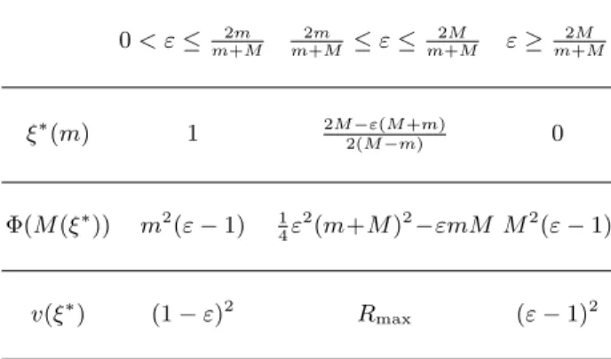
Lemma 1.Let 0 < m < M, ε > 0 and let ξ∗ be the optimum design
corre-sponding to the optimality criterion(1.25). Then ξ∗is supported at two points
Table 1.2. Values of ξ∗(m), Φ(M (ξ∗)) and v(ξ∗) 0 < ε ≤ 2m m+M 2m m+M ≤ ε ≤ 2M m+M ε ≥ 2M m+M ξ∗(m) 1 2M −ε(M+m) 2(M −m) 0 Φ(M (ξ∗)) m2(ε − 1) 1 4ε 2(m+M )2−εmM M2(ε − 1) v(ξ∗) (1 − ε)2 R max (ε − 1)2
The proof is straightforward.
In addition to the values of the weights ξ∗(m), Table 1.2 contains the values of the optimality criterion Φ(M (ξ)) and the rate function v(ξ) for the optimum design ξ = ξ∗.
Theorem 1 below shows that if the relaxation coefficient ε is either small (ε < 4M m/(M + m)2) or large (ε > 1), then for almost all starting points
the algorithm asymptotically behaves as if it has started at the worst possible initial point. However, for some values of ε the rate does not attract to a constant value and often exhibits chaotic behaviour. Typical behaviour of the asymptotic rate (1.5) is shown in Fig. 1.1 where we display the asymptotic rates in the case M/m = 10.
In this figure and all other figures in this chapter we assume that d = 100 and all the eigenvalues are equally spaced. We have established numerically that the dependence on the dimension d is insignificant as long as d ≥ 10. In particular, we found that there is virtually no difference in the values of the asymptotic rates corresponding to the cases d = 100 and d = 106, for
all the algorithms studied. In addition, choosing equally spaced eigenvalues is effectively the same as choosing eigenvalues uniformly distributed on [m, M ] and taking expected values of the asymptotic rates.
Theorem 1.Assume that ε is such that either 0 < ε < 4M m/(m + M )2 or ε > 1. Let ξ0 be any non-degenerate probability measure with support
{λ1, . . . , λd} and let the sequence of probability measures {ξ(k)} be defined
via the updating formula (1.24) where p(k)i are the massesξ(k)(λ
i). Then the following statements hold:
• for any starting point x0, the sequence Φk = Φ(M (ξ(k))) monotonously
increases(Φ0≤Φ1≤· · ·≤Φk ≤· · · ) and converges to a limit limk→∞Φk.
• For almost all starting points x0 (with respect to the uniform distribution ofg0/p||g0|| on the unit sphere in Rd),
1 Studying convergence of gradient algorithms 13
Fig. 1.1.Asymptotic rate of convergence as a function of ε for the steepest-descent algorithm with relaxation ε
equal toΦ(M (ξ∗)) as defined in Table 1.2;
– the sequence of probability measures{ξ(k)} converges (as k → ∞) to the
optimum designξ∗ defined in Lemma 1, and
– the asymptotic rateR of the steepest-descent algorithm with relaxation,
as defined in (1.2) and (1.23), is equal to v(ξ∗) defined in Table 1.2.
Proof. Note that Φk ≤ 0 for all ξ(k) if
0 < ε < min ξ µ2 1(ξ) µ2(ξ) = 4M m (m + M )2.
If ε ≥ 1 then Φk ≥ 0 for any ξ(k) in view of the Cauchy–Schwarz inequality.
Additionally, |Φk| ≤ (1 + ε)M2 for all ξ(k)so that {Φk} is always a bounded
sequence.
The updating formulae for the moments are µ′1= (µ31− 2εµ1µ2+ ε2µ3)/W and µ ′ 2= (µ21µ2− 2εµ1µ3+ ε2µ4)/W where W = ε2µ 2+ µ21(1 − 2ε) and µα= µα(ξ(k)), µ ′ α= µα(ξ(k+1)), ∀α, k = 0, 1, . . . (1.26)
The sequence Φk is non-decreasing if Φk+1− Φk ≥ 0 holds for any
prob-ability measure ξ = ξ(k). If for some k the measure ξ(k) is degenerate (that
theorem holds. Let us suppose that ξ = ξ(k) is non-degenerate for all k. In
particular, this implies µ2> µ21and
W = ε2µ2+ µ21(1 − 2ε) = µ21(1 − ε)2+ ε2(µ2− µ21) > 0 . We have: Φk+1− Φk ≥ 0 ⇐⇒ ³ εµ′2− (µ ′ 1)2 ´ −³εµ2− µ21 ´ ≥ 0 . (1.27) We can represent the left-hand side of the second inequality in (1.27) as
³ εµ′2− (µ ′ 1)2 ´ −³εµ2− µ21 ´ = ε U W2, where U = W (µ21µ2− 2εµ1µ3+ ε2µ4− W µ2) + (W µ1+ µ31− 2εµ1µ2+ ε2µ3)(εµ1µ2− εµ3− 2 µ13+ 2 µ1µ2) .
As W2 will always remain strictly positive, the problem is reduced to deter-mining whether or not U ≥ 0. To establish the inequality U ≥ 0, we show that U = V (a, b) for some a and b, where
V(a, b) = var(aX +bX2) = a2µ2+ 2abµ3+b2µ4−(aµ1+bµ2)2≥ 0 (1.28)
and X is the random variable with distribution ξ.
Consider U − V (a, b) = 0 as an equation with respect to a and b and prove that there is a solution to this equation. First, choose b to eliminate the µ4
term: b = b0= ε
√
W . The value of b0 is correctly defined as W > 0.
The next step is to prove that there is a solution to the equation U − V (a, b0) = 0 with respect to a. Note that U − V (a, b0) is a quadratic function
in a. Let D be the discriminant of this quadratic function; it can be simplified to
D = (ε − 1)¡εµ2− µ12¢ ¡µ3ε + 2 µ13− εµ1µ2− 2 µ2µ1¢ 2
.
This is clearly non-negative for ε > 1 and 0 < ε < 4M m/(m + M )2. Therefore, there exist some a and b such that U = V (a, b). This implies Φk+1− Φk ≥ 0
and therefore {Φk} is a monotonously increasing bounded sequence converging
to some limit Φ∗= limk→∞Φk.
Consider now the second part of the theorem. Assume that the initial measure ξ0 is such that ξ0(m) > 0 and ξ0(M ) > 0.
From the sequence of measures {ξ(k)} choose a subsequence weakly
con-verging to some measure ξ∗ (we can always find such a sequence as all the measures are supported on an interval). Let X = X∗ be the random variable defined by the probability measure ξ∗. For this measure, the value of V defined in (1.28) is zero as Φ(M (ξ(k+1))) = Φ(M (ξ(k))) if ξ(k) = ξ
∗. Therefore, the
1 Studying convergence of gradient algorithms 15
and therefore X∗ is concentrated at either a single point or at two distinct
points.
Assume that ε < 1 and therefore 0 < ε < 4M m/(m + M )2 (similar
arguments work in the case ε > 1). Then, similar to the proof for the steepest-descent algorithm (see (Pronzato et al., 2000, p. 175)) one can see that the masses ξ(k)(m) are bounded away from 0; that is, ξ(k)(m) ≥ c for some c > 0 and all k, as long as ξ0(m) > 0. Therefore, the point m always belongs to the
support of the measure ξ∗. If 0 < ε < 2m/(m + M ) then one can easily check that ξ∗ must be concentrated at a single point (otherwise U = U (ξ∗) 6= 0); this point is necessarily m and therefore the limiting design ξ∗coincides with the optimal design ξ∗. If 2m/(m + M ) < ε < 4M m/(m + M )2, then using
similar arguments one can find that the second support point of ξ∗ is M for almost all starting points.1As long as the support of ξ
∗is established, one can
easily see that the only two-point design that has U (ξ∗) = 0 is the optimal design ξ∗ with respect to the criterion (1.25).
One of the implications of the theorem is that if the relaxation parameter is either too small (ε < 2m/(m + M )) or too large (ε > 2M/(m + M )) then the rate of the steepest-descent algorithm with relaxation becomes worse than Rmax, the worst-case rate of the standard steepest-descent algorithm.
As a consequence, we also obtain a well-known result that if the value of the relaxation coefficient is either ε < 0 or ε > 2, then the steepest descent with relaxation diverges. When 4M m/(m + M )2 < ε ≤ 1 the relaxed
steepest-descent algorithm does not necessarily converge to the optimum design. It is within this range of ε that improved asymptotic rates of convergence are demonstrated, see Fig. 1.1.
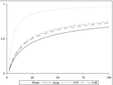
The convergence rate of all gradient-type algorithms depends on, amongst other things, the condition number ̺ = M/m. As one would expect, an in-crease in ̺ gives rise to a worsened rate of convergence. The improvement yielded by the addition of a suitable relaxation coefficient to the steepest-descent algorithm however, produces significantly better asymptotic rates of convergence than standard steepest descent. Fig. 1.2 shows the effect of in-creasing the value of ̺ on the rates of convergence for the steepest-descent al-gorithm with relaxation coefficients ε = 0.97 and ε = 0.99 (see also Fig. 1.10). For large d and ̺, we expect that the asymptotic convergence rates for this family of algorithms will be bounded above by Rmaxand below by Rminwhere
Rmin= Ã√ M −√m √ M +√m !2 = Ã√ ̺ − 1 √̺ + 1 !2 ; (1.29)
1 The only possibility for M to vanish from the support of the limiting design ξ ∗
is to obtain µ1(ξ(k))/ε = M at some iteration k, but this obviously almost never
(with respect to the distribution of g0/p||g0||) happens. Note that in this case M
will be replaced with λd−ifor some i ≥ 1 which can only improve the asymptotic
the rate Rmin is exactly the same as the rate N∞∗ defined in (3.22), Chap. 3.
The relaxation coefficient ε = 0.99 produces asymptotic rates approaching Rmin, see also Fig. 1.10).
Fig. 1.2. Asymptotic rate of convergence as a function of ̺ for steepest descent with relaxation coefficients ε = 0.97 and ε = 0.99
In Fig. 1.3 we display 250 rates v(ξk), 750 < k ≤ 1000 which the
steepest-descent algorithms with relaxation coefficients ε ∈ [0.4, 1] attained starting at the random initial designs ξ0. In this figure, we observe bifurcations and
transitions to chaotic regimes occurring for certain values of ε.
Fig. 1.4 shows the same results but in the form of the log-rates, − log(v(ξk)).
Using the log-rates rather than the original rates helps to see the variety of small values of the rates, which is very important as small rates v(ξk) force
the final asymptotic rate to be small.
Fig. 1.5 shows the log-rates, − log(v(ξk)), occurring for ε ∈ [0.99, 1.0]. This
figure illustrates the effect of bifurcation to chaos when we decrease the values of ε starting at 1.
1.8 Square-root algorithm
For the square-root algorithm, we have:
Φ(M (ξ)) =√µ2− µ1, v = v(ξ) = 2(1 −
µ1
õ
2
) .
In the present case, the optimum design ξ∗ is concentrated at the points
1 Studying convergence of gradient algorithms 17 0.4 0.5 0.6 0.7 0.8 0.9 1 0 0.4 0.8 1.2 1.6 2
Fig. 1.3.Rates v(ξk) (750 < k ≤ 1000) for steepest descent with relaxation; varying
ε, ̺ = 10 0.4 0.5 0.6 0.7 0.8 0.9 1 0 2 4 6 8
Fig. 1.4. Log-rates − log(v(ξk)) (750 < k ≤ 1000) for steepest descent with
relax-ation; varying ε, ̺ = 10
ξ∗(M ) = 3m + M 4(m + M ), ξ
∗(m) = m + 3M
4(m + M ). (1.30) For the optimum design, we have
0.99 0.992 0.994 0.996 0.998 1 0 2 4 6 8 10 12
Fig. 1.5. Log-rates − log(v(ξk)) (750 < k ≤ 1000) for steepest descent with
relax-ation; ̺ = 10, ε ∈ [0.99, 1.0] Φ(M (ξ∗)) = 1 4 (M − m)2 m + M and v(ξ ∗) = R max.
The main updating formula (1.7) has the form
p(k+1)i = (1 − √1 µ2λi) 2 2(1 −√µ1µ2) p (k) i . (1.31)
Theorem 2.Let ξ0 be any non-degenerate probability measure with support {λ1, . . . , λd} and let the sequence of probability measures {ξ(k)} be defined
via the updating formula (1.31) where p(k)i are the massesξ(k)(λ
i). Then the following statements hold:
• for any starting point x0, the sequence Φk = Φ(M (ξ(k))) monotonously
increases(Φ0≤Φ1≤· · ·≤Φk ≤· · · ) and converges to a limit limk→∞Φk.
• If the starting point x0of the optimization algorithm is such thatξ(0)(λ1) >
0 and ξ(0)(λ
d) > 0, then
– the limit limk→∞Φk does not depend on the initial measureξ(0) and is
equal toΦ(M (ξ∗)) = (M − m)2/[4(m + M )];
– the sequence of probability measures{ξ(k)} converges (as k → ∞) to the
optimum designξ∗ defined in (1.30), and
– the asymptotic rateR of the square-root optimization algorithm is equal
toRmax.
Proof. The proof is similar to (and simpler than) the proof of Theorem 1.
1 Studying convergence of gradient algorithms 19 µ′1= µ µ1− 2√µ2+ µ3 µ2 ¶ /v , µ′2= µ µ2− 2 µ3 √µ 2 + µ4 µ2 ¶ /v ,
where we use the notation for the moments introduced in (1.26). Furthermore, Φk+1− Φk= q µ′ 2− µ ′ 1−√µ2+ µ1, Φk+1≥ Φk ⇐⇒ q µ′ 2≥ µ ′ 1+√µ2− µ1= µ3− µ1µ2 2√µ2¡√µ2− µ1¢− µ 1. The inequality µ′2≥ (µ ′ 1+√µ2− µ1)2 (1.32)
would therefore imply Φk+1≥ Φk for any design ξ = ξ(k).
Let X be a random variable with probability distribution ξ = ξk. Then we
can see that the difference µ′2− (µ ′ 1+ √µ2− µ1)2 can be represented as µ′2− (µ ′ 1+√µ2− µ1)2= 1 2√µ2(√µ2− µ1) var(aX + X2) ≥ 0 where a = κ + κ + 2√µ√ 2 2 r 1 −√µµ1 2 and κ =µ1µ2− µ3 µ2− µ21 .
This implies (1.32) and therefore the monotonic convergence of the sequence {Φk}.
As a consequence, any limiting design for the sequence {ξk} is concentrated
at two points. If ξ(0)(λ
1) > 0 and ξ(0)(λd) > 0, then there is a constant c0
such that ξ(k)(λ
1) > c0 and ξ(k)(λd) > c0for all k implying that the limiting
design is concentrated at m and M . The only design with support {m, M} that leaves the value of Φ(M (ξ)) unchanged is the optimal design ξ∗ with
weights (1.30). The rate v(ξ∗) for this algorithm is R max.
1.9 A-optimality
Consider the behaviour of the gradient algorithm generated by the A-optimality criterion in the two-dimensional case; that is, when d = 2, λ1 = m and
λ2= M . Assume that the initial point x0 is such that 0 < ξ(0)(m) < 1
(oth-erwise the initial design ξ(0) is degenerated and so are all other designs ξ(k),
k ≥ 1).
Denote pk = ξ(k)(m) for k = 0, 1, . . .. As d = 2, all the designs ξ(k) are
fully described by the corresponding values of pk. In the case of A-optimality,
f (p) = Ã 1 − ¡1 + µ1 2¢ µ1(1 + µ2) m !2 µ12(1 + µ2)2 (1 + 2 µ12+ µ12µ2) (µ2− µ12) p ,
µ1 = pm + (1 − p)M and µ2 = pm2+ (1 − p)M2. The fixed point of the
transformation pk+1= f (pk) is
p∗=
M2+ 1 −p(M2+ 1)(m2+ 1)
M2− m2 .
For this point we have p∗= f (p∗) and the design with the mass p∗ at m and
mass 1 − p∗ at M is the A-optimum design for the linear regression model
yj = θ0+ θ1xj+ εj on the interval [m, M ] (and any subset of this interval that
includes m and M ). This fixed point p∗ is unstable for the mapping p → f(p)
as |f′(p∗)| > 1.
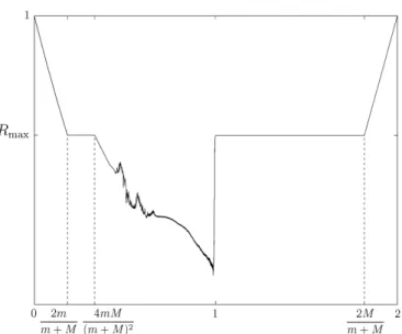
For the transformation f2(·) = f(f(·)), see Fig. 1.6 for an illustration of
this map, there are two stable fixed points which are 0 and 1. The fact that the points 0 and 1 are stable for the mapping p → f2(p) follows from
(f (f (p)))′ ¯ ¯ ¯ ¯p=0 = (f (f (p)))′ ¯ ¯ ¯ ¯p=1 = f′(0)f′(1) = (M m + 1) 4 (m2+ 1)2(M2+ 1)2;
the right-hand side of this formula is always positive and less than 1. There is a third fixed point for the mapping p → f2(p); this is of course p
∗ which is
clearly unstable.
1 Studying convergence of gradient algorithms 21 0.8 1.2 1.6 2 0.6 0.7 0.8 0.9 1 0.8 1.2 1.6 2 0.7 0.8 0.9 1
Fig. 1.7. Asymptotic rates for the α-root gradient algorithm; left: ̺ = 50, right: ̺ = 100
This implies that in the two-dimensional case the sequence of measures ξ(k) attracts (as k → ∞) to a cycle of oscillations between two degenerate
measures, one is concentrated at m and the other one is concentrated at M . The superlinear convergence of the corresponding gradient algorithm follows from the fact that the rates v(ξ) at these two degenerate measures are 0 (implying vk → 0 as k → ∞ for the sequence of rates vk).
To summarize the result, we formulate it as a theorem.
Theorem 3.For almost all starting pointsx0, the gradient algorithm
corre-sponding to theA-optimality criterion for d = 2 has a superlinear convergence
in the sense that the sequence of ratesvk tends to0 as k → ∞.
If the dimension d is larger than 2, then the convergence of the optimiza-tion algorithm generated by the A-criterion is no longer superlinear. In fact, the algorithm tries to attract to the two-dimensional plane with the basis e1, ed by reducing the weights of the designs ξ(k) at the other eigenvalues.
However, when it gets close to the plane, its convergence rate accelerates and the updating rule quickly recovers the weights of the other components. Then the process restarts basically at random, which creates chaos. (This phe-nomenon is observed in many other gradient algorithms with fast asymptotic convergence rate.)
The asymptotic rate (in the form of efficiency with respect to Rmin) of the
gradient algorithm generated by the A-criterion, is shown in Fig. 1.10.
1.10 α-root algorithm and comparisons
In Fig. 1.7 we display the numerically computed asymptotic rates for the α-root gradient algorithm with α ∈ [0.75, 2], ̺ = 50 and ̺ = 100. This figure illustrates that for α < 1 the asymptotic rate of the algorithm is Rmax. The
Numerical simulations show that the optimal value of α depends on ̺ and on the intermediate eigenvalues. For ̺ ≤ 85 the optimal value of α tends to be around 1.015; for ̺ = 90 ± 5 the optimal value of α switches to a value of around 1.05, where it stays for larger values of ̺.
In Fig. 1.8 we display 250 log-rates, − log(v(ξk)), 750 < k ≤ 1000, which
the α-root gradient algorithm attained starting at the random initial design ξ0, for different α. This figure is similar to Fig. 1.4 for the steepest-descent
algorithm with relaxation.
Fig. 1.9 is similar to Fig. 1.5 and shows the log-rates, − log(v(ξk)), for the
α-root gradient algorithm occurring for α ∈ [1.0, 1.01].
1 1.1 1.2 1.3 1.4 1.5 0 4 8 12 16
Fig. 1.8.Log-rates − log(v(ξk)) (750 < k ≤ 1000) for the α-root gradient algorithm;
varying α, ̺ = 10
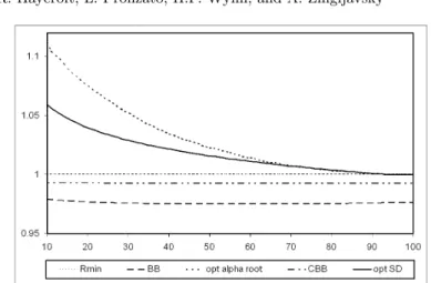
In Fig. 1.10 we compare the asymptotic rates of the following gradient algorithms: (a) α-root algorithm with α = 1.05; (b) the algorithm based on the Φ2-optimality criterion, see (1.22); (c) steepest descent with relaxation
ε = 0.99, see Sect. 1.7, and (d) the algorithm based on A-optimality criterion, see Sect. 1.9. The asymptotic rates are displayed in the form of efficiencies with respect to Rminas defined in (1.29); that is, as the ratios Rmin/R, where
R is the asymptotic rate of the respective algorithm.
In Fig. 1.11 we compare the asymptotic rates (in the form of efficiencies with respect to Rmin) of the following gradient algorithms: (a) α-root
algo-rithm with optimal value of α; (b) steepest descent with optimal value of the relaxation coefficient ε; (c) Cauchy–Barzilai–Borwein method (CBB) as de-fined in (Raydan and Svaiter, 2002); (d) Barzilai–Borwein method (BB) as defined in (Barzilai and Borwein, 1988).
1 Studying convergence of gradient algorithms 23 1.0 1.002 1.004 1.006 1.008 1.01 0 2 4 6 8
Fig. 1.9. Log-rates − log(v(ξk)) (750 < k ≤ 1000) the α-root gradient algorithm;
̺ = 10, α ∈ [1.0, 1.01]
Fig. 1.10.Efficiency relative to Rminfor various algorithms, varying ̺
References
Akaike, H. (1959). On a successive transformation of probability distribution and its application to the analysis of the optimum gradient method. Ann. Inst. Statist. Math. Tokyo, 11, 1–16.
Barzilai, J. and Borwein, J. (1988). Two-point step size gradient methods. IMA Journal of Numerical Analysis, 8, 141–148.
Fig. 1.11.Efficiency relative to Rminfor various algorithms, varying ̺ (other
algo-rithms)
Forsythe, G. (1968). On the asymptotic directions of the s-dimensional optimum gradient method. Numerische Mathematik, 11, 57–76.
Kozjakin, V. and Krasnosel’skii, M. (1982). Some remarks on the method of minimal residues. Numer. Funct. Anal. and Optimiz., 4(3), 211–239.
Nocedal, J., Sartenaer, A., and Zhu, C. (2002). On the behavior of the gradient norm in the steepest descent method. Computational Optimization and Applications, 22, 5–35.
Pronzato, L., Wynn, H., and Zhigljavsky, A. (2000). Dynamical Search. Chapman & Hall/CRC, Boca Raton.
Pronzato, L., Wynn, H., and Zhigljavsky, A. (2001). Renormalised steepest descent in Hilbert space converges to a two-point attractor. Acta Applicandae Mathe-maticae, 67, 1–18.
Pronzato, L., Wynn, H., and Zhigljavsky, A. (2002). An introduction to dynamical search. In P. Pardalos and H. Romeijn, editors, Handbook of Global Optimization, volume 2, Chap. 4, pages 115–150. Kluwer, Dordrecht.
Pronzato, L., Wynn, H., and Zhigljavsky, A. (2006). Asymptotic behaviour of a fam-ily of gradient algorithms in Rdand Hilbert spaces. Mathematical Programming,
A107, 409–438.
Raydan, M. and Svaiter, B. (2002). Relaxed steepest descent and Cauchy-Barzilai-Borwein method. Computational Optimization and Applications, 21, 155–167.

![Fig. 1.5. Log-rates − log(v(ξ k )) (750 < k ≤ 1000) for steepest descent with relax- relax-ation; ̺ = 10, ε ∈ [0.99, 1.0]](https://thumb-eu.123doks.com/thumbv2/123doknet/13006082.380284/19.892.233.641.120.444/fig-log-rates-steepest-descent-relax-relax-ation.webp)
![Fig. 1.9 is similar to Fig. 1.5 and shows the log-rates, − log(v(ξ k )), for the α-root gradient algorithm occurring for α ∈ [1.0, 1.01].](https://thumb-eu.123doks.com/thumbv2/123doknet/13006082.380284/23.892.264.634.351.650/fig-similar-fig-shows-rates-gradient-algorithm-occurring.webp)