HAL Id: hal-02632523
https://hal.inrae.fr/hal-02632523
Submitted on 27 May 2020HAL is a multi-disciplinary open access
archive for the deposit and dissemination of sci-entific research documents, whether they are pub-lished or not. The documents may come from teaching and research institutions in France or
L’archive ouverte pluridisciplinaire HAL, est destinée au dépôt et à la diffusion de documents scientifiques de niveau recherche, publiés ou non, émanant des établissements d’enseignement et de recherche français ou étrangers, des laboratoires
Scale sensitivity and question order in the contingent
valuation method
Henrik Andersson, Mikael Svensson
To cite this version:
Henrik Andersson, Mikael Svensson. Scale sensitivity and question order in the contingent valuation method. Journal of Environmental Planning and Management, Taylor & Francis (Routledge): STM, Behavioural Science and Public Health Titles, 2014, 57 (11), pp.1746-1761. �10.1080/09640568.2013.839442�. �hal-02632523�
Scale sensitivity and question order in the contingent valuation method
Henrik Andersson1, *, Mikael Svensson21 Toulouse School of Economics (LERNA, UT1C, CNRS), Toulouse, France 2 Department of Economics, Karlstad University, Sweden
*
To whom correspondence should be addressed. Corresponding address: Toulouse School of Economics (LERNA), 21 all.de Brienne, 31015 Toulouse Cedex 6,
France, e-mail: henrik.andersson@tse-fr.eu
Acknowledgements Financial support from VTI, the Centre for Transport Studies, Stockholm, and
the Swedish Civil Contingencies Agency is gratefully acknowledged. The authors would also like to express their gratitude to two anonymous reviewers for their helpful comments on an earlier draft. The usual disclaimers apply.
Abstract: This study examines the effect on respondents' willingness to pay to reduce mortality
risk by the order of the questions in a stated preference study. Using answers from an experiment conducted on a Swedish sample where respondents’ cognitive ability was measured and where they participate in a contingent valuation survey it is found that scale sensitivity is the strongest when respondents are asked about a smaller risk reduction first (“Bottom-up” approach). This contradicts some previous evidence in the literature. It is also found that the respondents’ cognitive ability is more important for showing scale sensitivity when respondents are asked about a larger risk reduction first (“Top-down” approach), also reinforcing the result that a “Bottom-up” approach is more consistent with answers in line with theoretical predictions for a larger part of respondents.
Keywords: Cognitive ability; Contingent valuation; Mortality risk; Order effect; Scale sensitivity JEL-Codes: D80; I10; Q51
Published as: Andersson, H., and M. Svensson: 2014, ‘Scale sensitivity and question order in the contingent valuation method’. Journal of Environmental Planning and Management 57(11), 1746-1761.
1. Introduction
Despite its increasing use in economic applications there is a longstanding critique of stated preference (SP) methods, such as the contingent valuation (CV) method, for being inadequate to measure individual preferences (Hausman 2012). In addition to the criticism that stated willingness to pay (WTP) usually is higher than observed WTP for the same good (List and Gallet 2001, Murphy, Allen et al. 2005), much of the criticism has been based on the lack of scale sensitivity (scale bias) found in many CV studies.1 Insensitivity to scale has particularly been
found in studies on “non-use values” and in studies valuing small changes in the probability of mortality and/or morbidity risks (Kahneman and Knetsch 1992, Desvouges, Johnson et al. 1993, Hammitt and Graham 1999). Lately, increasing criticism has also surrounded the presence of order effects in CV studies (Bateman and Langford 1996, Powe and Bateman 2003, Clark and Friesen 2008); that stated WTP is dependent upon in which order the WTP questions are shown to the respondent.
Advocates of CV studies argue that the lack of scale sensitivity and the presence of order effects are results of bad survey design (Smith 1992, Carson and Mitchell 1995, Carson, Flores et al. 2001). Critics, however, argue that biases in CV studies can be explained by anomalies and cognitive constraints among respondents resulting in reference dependent and non-stable preferences (Kahneman and Knetsch 1992, Desvouges, Johnson et al. 1993, Diamond and Hausman 1994, Kahneman, Ritov et al. 1999). Particularly regarding studies eliciting WTP for small changes in mortality risk, used to estimate the value of a statistical life (VSL), cognitive constraints have been argued to be particularly important to understand the lack of scale sensitivity (Corso, Hammitt et al. 2001, Alberini, Cropper et al. 2004, Andersson and Svensson 2008). In a previous paper we showed that respondents who scored higher on a simple test of cognitive ability were more likely to give WTP responses for mortality risk reductions that were
1 Scale and scope are used interchangeably in the literature to define the size of the good. Here we have
in line with theoretical predictions, i.e. showing scale sensitivity (Andersson and Svensson 2008). A recent study also indicated that anchoring, i.e. that WTP can be manipulated by an uninformative anchor, was less pronounced among respondents with higher cognitive ability (Bergman, Ellingsen et al. 2010).
In a recent study merging the literature on scale bias and order effects, Nielsen and Kjaer (2011) examined if the question order influenced sensitivity to scale in people’s valuation of increased life expectancy in an air pollution context. They found a higher scale sensitivity when respondents were asked about the larger risk reduction first (“Top-down”). The approach of this paper is similar to the one in Nielsen and Kjaer (2011) but adds a focus and interaction with the cognitive ability of respondents. Hence, we merge the literature on scale bias and order effects with a particular focus on a potential interaction with cognitive ability. The latter is particularly relevant seen in the light of the arguments that biases in CV studies can be explained by cognitive constraints among respondents. Specifically, in this paper we address the following research questions:
(1) Does the order of questions affect the WTP for mortality risk reductions in a CV study?
(2) Is scale sensitivity affected by the order of WTP questions?
(3) Does cognitive ability have an effect on potential order effects and scale sensitivity? The research questions are analyzed based on a CV study on respondents’ WTP for mortality risk reductions that was conducted jointly with a brief test of their cognitive ability. The rest of the paper is structured as follows. In the following section we present the theoretical model and methodological considerations relevant to our research questions. Section 3 describes the survey and data collection. The results are shown in section 4, while section 5 ends the paper with a discussion and some concluding remarks.
2. Methodological Issues
2.1 Marginal willingness to pay to reduce mortality risk and scale sensitivity
The valuation task in this paper consists of estimating respondents’ marginal WTP to reduce mortality risk, which usually is denoted the value of a statistical life (VSL). VSL is a measure of the population mean marginal rate of substitution between mortality risk and wealth (Dreze 1962, Schelling 1968). The decision individuals face can be illustrated with a state-dependent expected utility model (Rosen 1988). Let w, p, andu ws
,s
a d, , denote wealth, baseline probability of death, and the state-dependent utilities, respectively, with subscripts a and d denoting survival and death. The survival lottery will then be given by:) ( ) 1 ( ) ( ) , (w p pu w p u w EU d a . (1)
For a marginal change of p we have the standard result that:
w p
u w u p w u w u dp dw VSL a d d a 1 constant EU , (2)where prime denotes first derivative (Hammitt 2000). Under the reasonable assumptions (which are standard in the literature) that u wa( )u w u wd( ), ( )a u wd( ) 0 andu ws( ) 0 for
,s a d , VSL is positive and increasing with w and p (Jones-Lee 1974, Weinstein, Shepard et al. 1980, Pratt and Zeckhauser 1996).
Equation (2) denotes “true” marginal WTP. In CV-studies respondents are asked to state their WTP for a small finite risk reduction, ∆p. VSL is then given by the ratio between the respondents’ maximum WTP and the risk reduction,
p WTP VSL
(3)
Equation (3) implies that WTP is proportional to the size of ∆p. The true relationship between WTP and the size of ∆p is only “near-proportional”, however. Near-proportionality is a necessary
(but not sufficient) condition for the WTP answers from CV studies to be valid estimates of individuals’ preferences (Hammitt 2000). The importance is evident from equation (3), since if WTP is not proportional to the size of ∆p then VSL will be highly sensitive to the choice of ∆p in a survey.
Hammitt (2000) proved this near-proportional relationship by examining the effect of the change in risk and wealth on VSL. The first effect, the change in risk, can be examined using equation (2). The effect on VSL from a small change in mortality risk ∆p will be less than or equal to 1/[1+∆p/(1-p)]. Since the baseline risk is usually quite small, a few percent or less, and since obviously ∆p<p, this effect is negligible (sometimes referred to as the “dead-anyway effect”). Regarding the second effect, the wealth effect, it is necessary to turn to the empirical evidence. The empirical evidence on the income elasticity of VSL suggests this elasticity to be between zero and one (Hammitt and Robinson 2011). Then, by using a numerical example Hammitt (2000) showed that WTP is nearly proportional to ∆p. It is important to keep in mind that near-proportionality requires that the baseline and the change in risk are small, and/or that the payment is not a substantial fraction of income.
Empirically, scale sensitivity may be divided into “weak” and “strong” scale sensitivity (Corso, Hammitt et al. 2001). Weak scale sensitivity is fulfilled if WTP increases with the size of the risk reduction, while strong scale sensitivity refers to the situation where WTP increases near-proportionally to the magnitude of the risk reduction. Earlier research has indicated that strong scale sensitivity is usually not met in CV studies valuing mortality risk reductions. For instance Hammitt and Graham (1999), found in their review of 25 studies that estimated WTP to protect or enhance human health or safety that most studies passed the weak scale sensitivity test, none passed the “strong” scale sensitivity test.
In empirical applications, scale sensitivity can be tested using either an internal (“within-sample”) test, which consists of asking a respondent two or more WTP questions with different sizes of the risk reduction, or an external (“between-sample”) test. The latter refers to varying the
size of the risk reduction to different groups of respondents where each respondent only answers one WTP question. In this study we conduct both internal and external tests of scale sensitivity.
2.2 Order effects
Order effects imply that the answer to the WTP question is affected by the order in which order the questions are asked. The theoretical expectations regarding if the order of questions should affect WTP depend on whether the valuation task is made from an inclusive or exclusive list (Bateman and Langford 1996). In inclusive lists, each subsequent good is described to be added to the previously valued good(s), while in exclusive lists goods are presented as alternatives to any other goods given in the list. Hence, in exclusive lists reference income, prices, quantity of goods consumed and utility level do not change across the valuation questions. Considering this, Bateman and Langford (1996) distinguish between theoretically expected “sequence effects” from inclusive lists due to income and substitution effects, and “order effects” from exclusive lists that are not consistent with theoretical predictions. Further, the literature has made a distinction between studies using advance disclosure or stepwise designs (Bateman, Cole et al. 2004). Advance disclosure refers to the situation where the respondent is being told up front about the different goods that are to be valued. In stepwise designs the respondent may first be asked to value good A, and only after that being told about good B, etc.
In this paper we focus on and test for order effects in exclusive lists with advanced disclosure, where economic theory does not predict any significant order effects to be present. Early studies on order effects in exclusive lists were Boyle, Reiling et al. (1990), Boyle, Welsh et al. (1993) who found some evidence for order effects (but not statistically significant in all tests). Later, Powe and Bateman (2003) asked respondents for their WTP for a prevention program of salt-water flooding of a smaller or a larger scale. They found that the smaller part program was valued significantly more highly if asked first (“Bottom-up”), rather than if asked after the larger part
(“Top-down”). There was also evidence that WTP for the larger good was higher in the “Bottom-up” approach. In the study by Bateman, Cole et al. (2004) they find significant order effects for a sample with stepwise designs, but no significant order effects in a sample with advance disclosure. For the smallest part of the good the mean WTP was highest in the “Bottom-up” approach, while the largest part of the good was highest in the “Top-down” approach.2 Recently,
Clark and Friesen (2008) test for order effects based on stepwise disclosure using an incentive-compatible Becker-DeGroot-Marschak mechanism for induced value goods, actual private goods and a private good being donated to charity. They find significant order effects for the private goods, such that both the smallest and largest good is valued higher in the “Bottom-up” approach. However, no order effect is found for the good being donated to charity. Moreover, they find no difference in scope sensitivity between the “Bottom-up” and the “Top-down” approach. Considering that Clark and Friesen (2008) report order effects also for the private good when elicited using incentive-compatible mechanisms may indicate that order effects are not something particularly associated with CV studies, but rather a general phenomenon also apparent in “real life decisions”.
Relatively similar to our study, Nielsen and Kjaer (2011) tested if the question order influenced sensitivity to scale in a valuation of increased life expectancy in an air pollution context. They find a higher degree of scale sensitivity in a “Top-down” approach, i.e. when the larger risk reduction is valued first. This is driven by the finding that the smaller risk reduction is valued relatively lower when asked second (whereas the valuation of the larger risk reduction does not differ significantly between the “Top-down” and “Bottom-up” approach).
2 Scale sensitivity is also tested by Bateman, Cole et al. (2004) and the results indicate scale sensitivity both
3. The experiment – cognitive ability and contingent valuation
In order to address the research questions we employ a CV survey on the WTP for a mortality risk reduction. The CV survey was part of an experiment conducted on 200 undergraduate students at Karlstad University in Sweden in the fall of 2005. The aim of the experiment was to examine how the respondents’ level of cognitive ability was correlated with WTP answers in line with predicted scale sensitivity. A positive correlation was found between cognitive ability and scale sensitivity. This paper focuses primarily on order effects on scale sensitivity and we refer to Andersson and Svensson (2008) for the analysis on cognitive ability and scale sensitivity.
Most of the students in the experiment were business majors (70 percent), but it also included students of economics, human resources, teaching and political science.3 The students were
recruited by being informed in class that they would be given the opportunity to take part in an experiment after the next lecture to provide valuable information for government authorities within the transport sector. They were informed that participation would be voluntary and that they would receive SEK 50 (ca. USD 7) as compensation for their participation.4 One person supervised the whole experiment and we therefore do not expect heterogeneity in the responses due to undue influence exerted by different interviewers.
The experiment contained a test of cognitive ability, the CV survey, and a number of background questions on respondents’ age, accident experience, etc. The test of cognitive ability consisted of 17 questions and was not in any way a complete test, but rather focused on skills in probabilities, syllogisms and computation. Hence, the test was a crude measure of cognitive ability but the questions used can be found in previous experiments and are similar to those used in intelligence tests (Kahneman and Tversky 1972, Kahneman and Tversky 1983, Rabin 2002, Frederick 2005). Individuals often make decisions based on heuristics (short cuts), since mental
3 Since a preliminary analysis showed that the area of study had no significant influence on the WTP
answers, this analysis based on area of study is omitted.
short cuts lighten the cognitive burden of decision-making (Kahneman, Slovic et al. 1982, Kahneman 2003), and the information from the test score is, therefore, valuable to test for a correlation between cognitive ability and order effects and scale sensitivity.5
In the CV part of the experiment respondents were randomly assigned to one out of four different treatments, where they were asked about their WTP to reduce the risk of being involved in a fatal bus accident. The respondents were each faced with two WTP questions, one for the smaller risk reduction ΔpS=4×10⁻⁵, and one for the larger ΔpL=6×10⁻⁵. It was clear beforehand to
respondents that they were to value two different risk reductions; an advanced disclosure approach. Since both samples were asked about the same risk reductions, the ratio between the risk reductions is equal for all respondents, i.e. 1.5. Moreover, to test for anchoring effects from the initial bus fare, half of the sample was told that the annual bus fare of the reference bus company was SEK 3,000, whereas the other half that it was SEK 4,200.6 Hence, in all, the
experiment consisted of four treatments based on question order and level of bus fare as summarized in Table 1.
[Table 1 about here]
Bus fatalities, which constitute ca. one percent of all road accident fatalities in Sweden (SIKA 2005), was chosen as the fatality risk for two reasons; familiarity and exogeneity. We assumed that the risk associated with using the bus would be both familiar and relevant to the students since many of the them need to use the bus to get to/from the city center of Karlstad and/or the campus at Karlstad University, which are located approximately 9 kilometers (ca. 5.6 miles) apart. Since the risk of riding a bus to a large extent is related to circumstances out of the
5 For a description of the test of cognitive ability and the questions used, see Andersson and Svensson
(2008). The design of the CV survey is available upon request from the authors.
passenger’s control, e.g. the condition of the bus, the driver's behavior, and other elements of the traffic situation, we believe that we have less problems of a risk perceived as endogenous. That is, we believe that respondents are more likely to perceive the risk as exogenous compared with a scenario where they would have been asked about, e.g., the risk while driving a car, riding a bike, or smoking, since in these scenarios they can influence the risk by their own skills. Before the WTP questions the respondents were informed about the overall mortality risk of a person in his/her 50s and of the average road-traffic fatality risk.7 The risks were visualized using a grid
containing of 10,000 whites squares where the appropriate number of squares had been blacked out to represent each risk. The visual aid was combined with a verbal probability analog for the road-fatality risk, since this combination has proved to provide answers more consistent with standard economic theory (Corso, Hammitt et al. 2001). The probability analog said that the risk was equivalent to eight individuals on average dying annually in road-traffic accidents in a city of the size of Karlstad. The first WTP question in Treatment 1 is illustrated in Figure 1. The open-ended format was chosen to avoid anchoring effects (Green, Jacowitz et al. 1998).
[Figure 1 about here]
The second question was identical to the first one except that Bus Company B (in Figure 1) had been replaced by another company C with a different risk level. To avoid a framing effect by letting respondents compare new bus companies with an existing one, all were presented as new companies, but with one as the reference.8 Following the CV survey, the experiment was
7The baseline risk of this particular age group was also used by Persson, Norinder et al. (2001) and Carlsson, Johansson-Stenman et al. (2004). We decided to use it since we wanted a baseline risk other than the respondents’ own age group to increase the chance of respondents perceiving the risks presented to them in the survey as exogenous.
8 The survey asks about the city council selecting from one of three bus companies that are distinguished by
the levels of safety, when contracting out the service to a private firm. This corresponds to the actual procedure in the city of Karlstad as well as most other Swedish cities.
concluded with a brief set of questions on some respondent individual characteristics (age, income, sex, etc.) and their accident experience.
4. Results9
4.1 Descriptive statistics
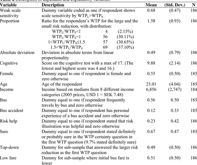
In total 14 respondents have been excluded from the sample since their WTP was equal to zero in either one (1 respondent) or both of the WTP questions (13 respondents). These respondents were excluded since it is not possible to test for internal scale sensitivity when at least one WTP answer is equal to zero. The descriptive statistics of the used sample is shown in Table 2 and many of the variables are self-explanatory but some may need further explanation. The variables
Weak scale sensitivity, Proportion and Absolute deviation in Table 2 indicate to what degree
respondents’ answers are in line with economic theory according to our hypotheses as outlined in section two. Weak scale sensitivity is a dummy variable which takes the value one if respondents state a higher WTP for the larger risk reduction than for the smaller one. Proportion is a measure of the ratio between the WTP for the larger and smaller risk reductions, and is equal to 1.5 for fourteen percent of the sample and has a mean value of 1.58, which is close to proportionality.
Absolute deviation is estimated as the absolute difference between the WTP ratio and
risk-reduction ratio. For instance, since the ratio between the risk risk-reductions is 1.5, a WTP ratio of 1.75 or 1.25 will mean an absolute deviation of 0.25. The mean score in the test on cognitive ability was close to 10, out of a maximum of 17, with a lowest and highest score equal to 4 and 16. We could not reject that the distribution of the test score was normal.
[Table 2 about here]
9 Since we use standard diagnostic tests and regression techniques we have not included a section where
these tests and techniques are described. For a description of the techniques, see any textbook on econometrics.
4.2 WTP and order effects
In Table 3 WTP for the small and large risk reduction are shown for the four treatments presented in Table 1, i.e. four subsamples based on the bottom-up or the top-down design for the WTP questions and with regards to the reference price of the bus fare in the survey (either “low fare” or “high fare”). The prediction from economic theory is that WTP for each risk reduction should be equal in the “Bottom-up” and “Top-down” approach for the low fare, high fare and pooled sample, respectively. The mean estimates shown in Table 3 are geometric means which are used to mitigate the effect from extreme values. The results seem to suggest that WTP is higher with the “Top-down” approach (Treatment 1 and 2), i.e. when the respondents value the larger risk reduction first, for the different risk reductions and reference prices. Indeed, for all treatments mean WTP is higher with the “Top-down” approach. However, the values are close and we do not find any statistically significantly difference in mean WTP for the same risk reductions in the four treatments. We, therefore, cannot reject equality of WTP between the “Bottom-up” and “Top-down” approach or between “Low fare” or “High fare”. Hence, based on these comparisons we do not find any evidence in favour of any anchoring effects on the level of WTP.
Since we do not find any framing effect from the reference prices we can pool treatments 1 and 2, and treatments 3 and 4. The mean WTP for these pooled treatments are shown at the bottom of Table 3 and again we cannot reject an absence of order effects. Moreover, we also run regression analyses where we tested for order and framing effects on respondents’ WTP. Again, we found no evidence of any order or framing effects, and since those results are in line with our findings in Table 3 they are not shown.10
[Table 3 about here]
4.3 Scale sensitivity and order effects
We start examining scale sensitivity by using the results from Table 3. By first examining the means and confidence intervals we find that the mean WTP of the first question is significantly different in the pooled treatments between the smaller (SEK 311.30) and large (SEK 499.85) risk reduction. All other confidence intervals are overlapping. However, our main analysis of Table 3 is based on non-parametric techniques; we employ the Mann-Whitney test for the external tests (i.e. between groups) and the Wilcoxon signed-rank test for internal tests.
Focusing first on external scale sensitivity we find for the pooled treatments that mean WTP for the two risk reductions is statistically significantly different at the 1% and 5% level for the first and second WTP question, respectively. When comparing the four treatments we find that the WTP for the larger risk reduction is significantly higher only for the first WTP question; it is statistically significantly different at the 5% level in the sample with the high fare, and at the 10% level in the sample with the low fare. For the second WTP question we do not find any difference at conventional significance levels. This could suggest, even if we cannot reject an absence of order effects, that respondents may have anchored their second WTP answer to their first one.
The internal test of weak scale sensitivity reveals that the null hypothesis of no scale sensitivity can be rejected at the 1% level for all treatments. Estimating the ratio between the WTP for the larger and the smaller risk reduction reveals a ratio that is higher with the “Bottom-up” compared with the “Top-down” approach. For instance, in the pooled sample the ratio for the respondents in the “Bottom-up” treatment is 1.35 (CI: 1.24 - 1.45) and for the “Top-down” treatment it is 1.23 (CI: 1.04 - 1.42). Using a non-parametric test we can reject equality of the two subsamples at the 10% level. Hence, the results in Table 3 provide some evidence that scale sensitivity is related to the order of the questions, with higher scale sensitivity in the “Bottom-up” approach.
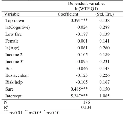
Before using regression analysis to examine scale sensitivity and order effects we examine the different covariates’ effect on WTP. The results are shown in Table 4 and in this regression we only use the respondents’ stated WTP to the first question. The reason is that this best reflects the analysis in a standard CV survey where often only one question is asked. Using only the first answer means that the test of scale sensitivity is an external test since the regression in Table 4 only includes information about each respondent’s WTP for one risk reduction. For the scale test we focus on the variable Top-down, which is the dummy equal to one for those respondents who answered the large valuation question first. The coefficient estimate for this variable is 0.391 and it is statistically significantly different from zero. A proportional WTP would result in a coefficient estimate equal to 0.405.11 A test shows that our estimate of 0.391 is not statistically
significantly different from 0.405 (p-value = 0.92). Thus, we can reject the null hypothesis of no scale sensitivity but not the one of a proportional WTP. Regarding the other covariates we only find a statistically significantly effect on WTP from Sure. This result suggests that those who are certain about their answer have a higher WTP (everything else equal). Follow-up preference certainty questions are usually not used in the open-ended format, but in the referendum format where respondents state whether they are willing to pay a specific bid or not for the good of interest, or to vote on a policy with the cost and the amount of the good well specified. Our result is not in line with the empirical findings using the referendum format which would suggest that respondents more certain about their answer in a hypothetical setting would have a lower WTP (e.g., Blumenschein, Blomquist et al. 2008). Theory predicts that WTP should increase with the wealth level. The reasons why we do not find this positive relationship could be because we have a student sample where current income is not a good predictor of lifetime income.
[Table 4 about here]
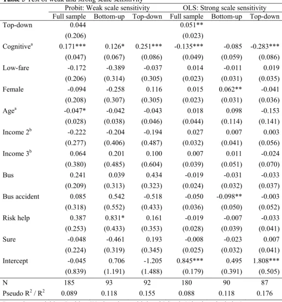
The result in Table 4 suggests that WTP is proportional to the size of the risk reduction. In a previous study analyzing the same data set it was shown, however, that scale sensitivity was related to the respondents’ score in the test on cognitive ability (Andersson and Svensson 2008). In Table 5 we extend their analysis by examining the effect on scale sensitivity from the order of the WTP questions. To test for weak scale sensitivity we run a probit model in which the dependent variable Weak scale sensitivity is equal to one if the respondent valued the larger risk reduction higher and zero otherwise. We use an OLS to test for strong scale sensitivity in which the dependent variable is the natural logarithm of the absolute deviation from proportionality.
Focusing on the regressions examining weak scale sensitivity we find in the regression on the full sample that the coefficient for the variable “Top-down” is positive, but not statistically significant. Hence, we cannot reject the null hypothesis that weak scale sensitivity does not differ between the “Top-down” and the “Bottom-up” approach. Regarding other results, we only find statistically significant coefficient estimates for Cognitive and Age; respondents with a better test score are more likely to show weak scale sensitivity, whereas age is negatively related. In column 3 and 4 the regression for weak scale sensitivity is run for the “Bottom-up” and “Top-down” subsamples, respectively. The results reveal that whereas respondents’ cognitive ability has a positive and statistically significant effect in both samples, it is higher in the “Top-down” sample.
[Table 5 about here]
Analyzing strong scale sensitivity we find for the full sample in column 5 that the deviation from proportionality is larger in the “Top-down” approach. Regarding other results, again we find a statistically significant correlation between scale sensitivity and cognitive ability, but no other covariates are statistically significant. The negative coefficient estimate suggests that the deviation from a proportional WTP is lower for respondents with a higher cognitive ability. Looking at separate regressions for the two subsamples (column 6 and 7), we find in the
“Bottom-up” sample that women’s deviation from proportionality is larger and that it is smaller among those who have experience from a bus accident. In the “Top-down” sample we find that the deviation from proportionality is smaller for those with a high score in the test on cognitive ability.
4.4 Cognitive ability and order effects and scale sensitivity
The results from our regression analyses suggest that, whereas cognitive ability has no effect on respondents’ WTP level, it has an effect on how sensitive their WTP is to the size of the risk reduction. That is, whereas we found no effect from cognitive ability on WTP in Table 4, we found in Table 5 that cognitive ability influence weak and strong scale sensitivity. In the full samples of Table 5 we find that respondents with a higher cognitive ability are more likely to show weak scale sensitivity and that their WTP is closer to being proportional to the size of the risk reduction.
Moreover, when splitting the sample according to the order of the WTP questions we find that the effect from cognitive ability on weak scale sensitivity is higher in the “Top-down” compared with the “Bottom-up” sample. The coefficients are not statistically significantly different, though. Overall the results suggest that weak scale sensitivity is related to respondents’ cognitive ability and they can be interpreted as cognitive ability being more important when respondents are first asked about the larger risk reduction. In the split sample test on strong scale sensitivity we find that cognitive ability only is related to the deviation from proportionality in the “Top-down” sample. Both coefficients are negative, but only the one in “Top-down” is
statistically significant and the coefficients are statistically significantly different at the 5% level. Thus, the result from the split sample analysis may imply that the cognitive task of evaluating health risks is harder when the first risk reduction is larger (“Top-down” approach).
5. Discussion
This article examines three main research questions: (1) testing for order effects in a CV study on the WTP for mortality risk reductions, (2) examining if the scale sensitivity in WTP for the two different risk reductions is affected by the order of the two WTP questions, and (3) examining the effect of cognitive ability on potential order effects and scale sensitivity.
Regarding the first research questions we showed in Table 3 that the raw data indicated that in the “Top-down” approach, i.e. asking for the larger risk reduction first, WTP was higher both for the larger and the smaller risk reduction. However, we do not find any statistically significantly differences when comparing the WTP for the same risk reductions in the different treatments, and we cannot reject equality of WTP between the “Bottom-up” and “Top-down” treatment. We used advanced disclosure in our survey, and the results of no order effects using advance disclosure is in line with the results in Bateman, Cole et al. (2004). In contrast to our results, Powe and Bateman (2003) found higher values in the “Bottom-up” approach, while Bateman, Cole et al. (2004) found higher values for the smallest good in the “Bottom-up” approach using stepwise design.
Conclusion 1: We cannot reject the hypothesis of no order effects in the CV study, i.e. WTP for mortality risk reductions is not significantly different between the “Top-down” and “Bottom-up” treatment.
For the second research question of scale sensitivity our main interest is in internal sensitivity, though we started out the analyses in section 4.3 by also applying some standard external tests of scale sensitivity. These tests revealed a WTP that was sensitive to the magnitude of the risk reduction and that proportionality was not rejected when the respondents’ first answer was used (Table 4). Hence, this external test suggested that the respondents’ WTP is in line with the theoretical predictions. But focusing more specifically on research question 2, in the analyses regarding internal scale sensitivity we found that scale sensitivity was higher among respondents
in the “Bottom-up” treatment and in the non-parametric test we rejected equality at the 10% level, giving some weak indications that the “Bottom-up” treatment is related to higher scale sensitivity closer to our theoretical predictions. However, controlling for other covariates (Table 5) does not give any indications that the “Bottom-up” treatment is related to higher scale sensitivity (we cannot reject equality between the two treatments). Continuing to the test for strong scale sensitivity (Table 5) we see that the absolute deviation from proportionality is higher in the “Top-down” treatment (p<0.05); yet again giving some indications that the Bottom-up treatment is related to answers more in line with our theoretical predictions. It should be noted that this result is opposite to the results presented in Nielsen and Kjaer (2011), who found a larger scale sensitivity in the “Top-down” approach.
Conclusion 2: We conclude that the “Bottom-up” treatment is related to answers closer to near-proportionality between the large and small mortality risk reduction. The answer regarding weak scale sensitivity is ambiguous, there are some indications that the “Bottom-up” treatment is related also to a higher weak scale sensitivity, but results are not robust and disappears when controlling for other covariates.
For the third research question we found that a higher cognitive ability was associated with a higher likelihood of showing weak scale sensitivity (Table 5), a general finding we have analysed in a previous paper (Andersson and Svensson 2008). Additionally, we show here that the general results holds at statistical significant levels in both treatments, with the effect slightly stronger in the “Top-down” treatment (Table 5). Further, we show that a higher score on the cognitive ability test was associated with a smaller deviation from the near-proportionality assumption in the full sample, but that this is driven by a significant effect in the Top-down treatment.
Conclusion 3: A higher cognitive ability is associated with a higher likelihood of showing weak scale sensitivity in both treatments, but the cognitive ability is only a significant factor for strong scale sensitivity in the “Top-down” treatment.
Additionally, other points worth mentioning are that bus mortality risk is not a pure private good, and there is a risk that values also represent paternalistic altruism (oriented to health) or that respondents answered strategically when they stated their WTP for that kind of risk reduction. Note that, since we conducted internal tests on scale sensitivity, our findings should not be affected by potential strategic bias, altruism, or whether stated WTP also reflects preferences to reduce injury risk (the respondent's answers should be affected to the same relative degree). Also, it should be kept in mind, though, that even if the sample was larger than is usually the case for experiments; the analysis was carried out based on a sample smaller than is usually the case for CV surveys. Finally, our experiment was carried out on a student sample which should be taken into consideration regarding generalizations of the results.
References
Alberini, A., M. Cropper, A. Krupnick and N. Simon (2004). "Does the value of a statistical life vary with age and health status? Evidence from the US and Canada." Journal of Environmental Economics and Management 48: 769-792.
Andersson, H. and M. Svensson (2008). "Cognitive Ability and Scale Bias in the Contingent Valuation Method." Environmental and Resource Economics 39: 481-495. Bateman, I., M. Cole, P. Cooper, S. Georgiou, D. Hadley and G. L. Poe (2004). "On visible choice sets and scope sensitivity." Journal of Environmental Economics and Management 47: 71-93.
Bateman, I. and I. H. Langford (1996). "Budget-constraint, temporal, and question-ordering effects in contingent valuation studies." Environmental Planning A 28: 1215-1228.
Baum, C. F. (2006). An Introduction to Modern Econometrics Using Stata. College Station, Texas, USA, Stata Press.
Bergman, O., T. Ellingsen, M. Johannesson and C. Svensson (2010). "Anchoring and Cognitive Ability." Economics Letters 107: 66-68.
Blumenschein, K., G. C. Blomquist, M. Johannesson, N. Horn and P. Freeman (2008). "Eliciting Willingness to Pay without Bias: Evidence from a Field Experiment." Economic Journal 118: 114-137.
Boyle, K. J., S. D. Reiling and M. L. Phillips (1990). "Species substitution and question sequencing in contingent valuation surveys evaluating the hunting of several types of wildlife." Leisure Sciences 12: 103-118.
Boyle, K. J., M. P. Welsh and R. D. Bishop (1993). "The role of question order and respondent experience in contingent valuation studies." Journal of Environmental Economics and Management 25: S80-S99.
Carlsson, F., O. Johansson-Stenman and P. Martinsson (2004). "Is Transport Safety More Valuable in the Air." Journal of Risk and Uncertainty 28(2): 147-163.
Carson, R. T., N. E. Flores and N. F. Meade (2001). "Contingent Valuation:
Controversies and Evidence " Environmental and Resource Economics 19(2): 173-210. Carson, R. T. and R. C. Mitchell (1995). "Sequencing and Nesting in Contingent Valuation Surveys." Journal of Environmental Economics and Management 28(2): 155-173
Clark, J. E. and L. Friesen (2008). "The causes of order effects in contingent valuation surveys: An experimental investigation " Journal of Environmental Economics and Management 56(2): 195-206.
Corso, P. S., J. K. Hammitt and J. D. Graham (2001). "Valuing Mortality-Risk
Reduction: Using Visual Aids to Improve the Validity of Contingent Valuation " Journal of Risk and Uncertainty 23(2): 165-184.
Desvouges, W. H., F. R. Johnson, R. W. Dunford, S. P. Hudson and K. N. Wilson (1993). Measuring Natural Resource Damage with Contingent Valuation: A Test of Validity and Reliability. Contingent Valuation: A Critical Assessment. J. A. Hausman. Amsterdam, North-Holland: 91-159.
Diamond, P. A. and J. A. Hausman (1994). "Contingent Valuation: Is Some Number Better than No Number?" Journal of Economic Perspectives 8(4): 45-64.
Dreze, J. H. (1962). "L'utilité sociale d'une vie humaine." Revue Francaise de Recherche Opérationnelle 22.
Frederick, S. (2005). "Cognitive Reflections and Decision Making." Journal of Economic Perspectives 19(4): 25-42.
Green, D., K. Jacowitz, D. L. McFadden and D. Kahneman (1998). "Referendum contingent valuation anchoring and willingness to pay for public goods." Resource and Energy Economics 20(2): 85-116.
Hammitt, J. K. (2000). "Evaluating Contingent Valuation on Environmental Health Risks: The Proportionality Test." AERE Newsletter 20(1): 14-19.
Hammitt, J. K. (2000). "Valuing Mortality Risk: Theory and Practice." Environmental Science & Technology 34(8): 1396-1400.
Hammitt, J. K. and J. D. Graham (1999). "Willingness to Pay for Health Protection: Inadequate Sensitivity to Probability?" Journal of Risk and Uncertainty 18(1): 33-62. Hammitt, J. K. and L. A. Robinson (2011). "The income elasticity of the value per statistical life: transferring estimates between high and low income populations." Journal of Benefit-Cost Analysis
2(1): Article 1.
Hausman, J. A. (2012). "Contingent Valuation: From Dubious to Hopeless." Journal of Economic Perspectives 26: 43-56.
Jones-Lee, M. W. (1974). "The Value of Changes in the Probability of Death or Injury " Journal of Political Economy, 82(4): 835-849.
Kahneman, D. (2003). "Maps of Bounded Rationality: Psychology for Behavioral Economics." American Economic Review 93(5): 1449-1475.
Kahneman, D. and J. L. Knetsch (1992). "Valuing public goods: The purchase of moral satisfaction." Journal of Environmental Economics and Management 22(1): 57-70. Kahneman, D., I. Ritov and D. Schkade (1999). "Economic preferences or Attitude Expressions?: An Analysis of Dollar Responses to Public Issues." Journal of Risk and Uncertainty 19(1-3): 203-235.
Kahneman, D., P. Slovic and A. Tversky (1982). Judgement under Uncertainty: Heuristics and Biases. Cambridge, Cambridge University Press.
Kahneman, D. and A. Tversky (1972). "Subjective Probability: A Judgement of Representativeness." Cognitive Psychology 3(3): 430-454.
Kahneman, D. and A. Tversky (1983). "Can irrationality be intelligently discussed?" Behavioral and Brain Sciences 6: 509-510.
List, J. A. and C. A. Gallet (2001). "What Experimental Protocol Influence Disparities Between Actual and Hypothetical Stated Values? ." Environmental and Resource Economics 20(3): 241-254.
Murphy, J., G. P. Allen, T. H. Stevens and D. Weatherhead (2005). "A Meta-analysis of Hypothetical Bias in Stated Preference Valuation " Environmental and Resource
Economics 30(3): 313-325.
Nielsen, J. S. and T. Kjaer (2011). "Does question order influence sensitivity to scope? Empirical findings from a web-based contingent valuation study." Journal of
Environmental Planning and Management (iFirst): 1-13.
Persson, U., A. Norinder, K. Hjalte and K. Gralén (2001). "The Value of a Statistical Life in Transport: Findings from a New Contingent Valuation Study in Sweden " Journal of Risk and Uncertainty 23(2): 121-134.
Powe, N. A. and I. Bateman (2003). "Ordering effects in nested 'top-down' and 'bottom-up' contingent valuation designs." Ecological Economics 45: 255-270.
Powe, N. A. and I. J. Bateman (2003). "Ordering effects in nested 'top-down' and 'bottom-up' contingent valuation designs." Ecological Economics 45: 255-270.
Pratt, J. W. and R. J. Zeckhauser (1996). "Willingness to Pay and the Distribution of Risk and Wealth " Journal of Political Economy 104(4): 747-763.
Rabin, M. (2002). "Inference by Believers in the Law of Small Numbers." Quarterly Journal of Economics 117(3): 775-816.
Rosen, S. (1988). "The Value of Changes in Life Expectancy." Journal of Risk and Uncertainty 1(3): 285-304.
Schelling, T. C. (1968). The Life You Save May Be Your Own. Problems in Public Expenditure Analysis. S. B. Chase. Washington D.C., The Brookings Institution: 127-162.
SIKA (2005). Vägtrafikskador.
Smith, V. K. (1992). "Arbitrary values, good causes, and premature verdicts." Journal of Environmental Economics and Management 22(1): 71-89.
Weinstein, M. C., D. S. Shepard and J. S. Pliskin (1980). "The Economic Value of Changing Mortality Probabilities: A Decision-Theoretic Approach." Quarterly Journal of Economics 94(2): 373-396.
Table 1 The experimental design
Treatments First good valued Second good valued
Reference bus price
Top-down treatment Treatment 1 Treatment 2 Δp=6×10Δp=6×10⁻⁵-5 Δp=4×10Δp=4×10⁻⁵-5 SEK SEK 3,000 4,200
Bottom-up treatment Treatment 3 Δp=4×10⁻⁵ Δp=6×10⁻⁵ SEK 3,000
Treatment 4 Δp=4×10⁻⁵ Δp=6×10⁻⁵ SEK 4,200
Table 2 Description of dependent and explanatory variables
Variable Description Mean (Std. Dev.) N
Weak scale sensitivity
Dummy variable coded as one if respondent shows scale sensitivity by WTPL>WTPS
0.68 (0.47) 186
Proportion Ratio for the respondent’s WTP for the large and the small risk reduction, with distribution:
1.58 (0.93) 186 WTPL/WTPS<1 WTPL/WTPS=1 1<WTPL/WTPS≤1.5 1.5<WTPL/WTPS 4 56 57 69 (2.15%) (30.11%) (30.65%) (37.10%) Absolute deviation Deviation in absolute terms from linear
proportionality
0.49 (0.79) 186
Cognitive Score on the cognitive test with a max of 17. (The
lowest and highest score was 4 and 16.) 9.88 (2.14) 186
Female Dummy equal to one if respondent is female and
zero otherwise
0.55 (0.50) 185
Age Age of the respondent 23.01 (4.04) 185
Income Income based on medians from 8 different income
categories (2005 prices, USD 1 = SEK 7.48)
6,856 (2,747) 184
Bus Dummy equal to one if respondent frequently
travels by bus and zero otherwise
0.56 0.50 185
Bus accident Dummy equal to one if respondent has personal
experience of a bus accident and zero otherwise 0.12 0.33 185
Risk help Dummy equal to one if respondent stated that risk illustration was helpful and zero otherwise
0.23 0.42 186
Sure Dummy equal to one if respondent stated definitely
or probably sure in the WTP certainty question in the first WTP question (9.7% stated definitely sure)
0.67 0.47 185
Top-down Dummy for sub-sample that answered the larger risk
reduction as the first WTP question
0.49 (0.50) 186
Low fare Dummy for sub-sample where initial bus fare is
lower
0.51 (0.50) 186
Table 3 Testing for order effects
Mean WTPb
Treatmenta Small risk reduction Large risk reduction N
Top-down treatment Treatment 1 326.79 (237.56 - 449.54) 432.88 (309.88 – 604.70) 46 Treatment 2 387.61 (279.44 – 537.66) 577.18 (422.72 – 788.09) 46 Bottom-up treatment Treatment 3 304.49 (220.21 – 421.03) 411.15 (299.27 – 564.87) 48 Treatment 4 318.57 (232.60 – 436.31) 462.64 (335.45 – 638.06) 46
Top-down treatment Treatments 1 + 2 355.90
(284.26 – 445.61)
499.85 (398.72 – 626.63)
92
Bottom-up treatment Treatments 3 + 4 311.30
(249.37 – 388.61) (348.85 – 543.89) 435.59 94
a: For a description of the treatments, see Table 1
b: Geometric mean with 95% conf. interval in parentheses
Tests: The internal (within-sample) and external (between-sample) tests of difference have been conducted
with the Wilcoxon signed-ranked and the Mann-Whitney test, respectively.
Results: (1) Framing effect of different bus fares not statistically significant. (2) Questions order effect on
WTP not statistically significant.
Table 4 Analysis of 1st WTP answer
Dependent variable:
ln(WTP Q1)
Variable Coefficient (Std. Err.)
Top-down 0.391*** 0.138 ln(Cognitive) 0.024 0.288 Low fare -0.177 0.139 Female 0.001 0.141 ln(Age) 0.061 0.260 Income 2a 0.105 0.189 Income 3a -0.095 0.231 Bus 0.046 0.143 Bus accident -0.125 0.226 Risk help -0.105 0.167 Sure 0.485*** 0.150 Intercept 5.247*** 1.065 N 176 R2 0.134 *** p<0.01, ** p<0.05, * p<0.10
Robust standard errors in parentheses.
To deal with observations considered as outliers or with high leverage we used DFITS statistics with a
cutoff value to remove observations equal to 2 / (see Baum 2006).
Test of proportionality, i.e. coefficient for Top-down = 0.405, p-value = 0.92.
a: The continuous variable Income has been replace a by group variable. Reference group is Income 1,
Table 5 Test of weak and strong scale sensitivity
Probit: Weak scale sensitivity OLS: Strong scale sensitivity
Full sample Bottom-up Top-down Full sample Bottom-up Top-down
Top-down 0.044 0.051** (0.206) (0.023) Cognitivea 0.171*** 0.126* 0.251*** -0.135*** -0.085 -0.283*** (0.047) (0.067) (0.086) (0.049) (0.059) (0.086) Low-fare -0.172 -0.389 -0.037 0.014 -0.011 0.019 (0.206) (0.314) (0.305) (0.023) (0.031) (0.035) Female -0.094 -0.258 0.116 0.015 0.062** -0.041 (0.208) (0.307) (0.305) (0.023) (0.031) (0.036) Agea -0.047* -0.042 -0.043 0.018 0.098 -0.153 (0.028) (0.038) (0.046) (0.044) (0.114) (0.141) Income 2b -0.222 -0.204 -0.194 0.027 0.007 0.003 (0.277) (0.406) (0.487) (0.032) (0.041) (0.056) Income 3b 0.064 0.201 0.100 0.007 0.011 -0.024 (0.380) (0.485) (0.604) (0.039) (0.051) (0.070) Bus 0.241 0.039 0.434 -0.019 -0.031 -0.033 (0.209) (0.313) (0.323) (0.024) (0.032) (0.037) Bus accident 0.085 0.542 -0.518 -0.050 -0.098** -0.003 (0.318) (0.552) (0.433) (0.036) (0.050) (0.052) Risk help 0.387 0.831* 0.161 -0.019 -0.007 -0.033 (0.253) (0.433) (0.353) (0.028) (0.039) (0.041) Sure -0.048 -0.461 0.193 -0.008 -0.023 0.007 (0.224) (0.319) (0.345) (0.025) (0.032) (0.041) Intercept -0.045 0.706 -1.205 0.845*** 0.495 1.808*** (0.839) (1.191) (1.488) (0.179) (0.391) (0.505) N 185 93 92 180 90 87 Pseudo R2 / R2 0.089 0.118 0.155 0.088 0.118 0.176
Dependent variables: Probit = Weak scale sensitivity, OLS = ln(Absolute deviation)
*** p<0.01, ** p<0.05, * p<0.10
Robust standard errors in parentheses.
To deal with observations considered as outliers or with high leverage in the OLS we used DFITS statistics with a cutoff value to remove observations equal to 2 / (see Baum 2006).
a: Natural logarithm of variables used in OLS regression
b: The continuous variable Income has been replace a by group variable. Reference group is Income 1,
Figures
Figure 1 Willingness to pay question with small risk reduction and low annual bus fare
We would first like to know how much you are willing to pay to travel with Bus company B instead of Bus company A. The risks of accidents with fatal outcome for Bus company A and B are:
Bus company A: Risk = 10 per 100,000 Bus company B: Risk = 6 per 100,000
An annual pass with Bus company A costs SEK 3,000 (SEK 250 × 12).
What is the maximum amount you are willing to pay more per year to travel with Bus company B instead of Bus company A?
The maximum amount I am willing to pay more is . . . SEK. Are you definitely sure, probably sure or unsure regarding your answer (mark with an x)?