HAL Id: halshs-03185520
https://halshs.archives-ouvertes.fr/halshs-03185520
Preprint submitted on 30 Mar 2021
HAL is a multi-disciplinary open access
archive for the deposit and dissemination of
sci-entific research documents, whether they are
pub-lished or not. The documents may come from
teaching and research institutions in France or
abroad, or from public or private research centers.
L’archive ouverte pluridisciplinaire HAL, est
destinée au dépôt et à la diffusion de documents
scientifiques de niveau recherche, publiés ou non,
émanant des établissements d’enseignement et de
recherche français ou étrangers, des laboratoires
publics ou privés.
Finding a needle in a haystack: Do Early Warning
Systems for Sudden Stops work?
Umberto Collodel
To cite this version:
Umberto Collodel. Finding a needle in a haystack: Do Early Warning Systems for Sudden Stops
work?. 2021. �halshs-03185520�
WORKING PAPER N° 2021 – 20
Finding a needle in a haystack:
Do EarlyWarning Systems for Sudden Stops work.
Umberto Collodel
JEL Codes:
Keywords: EarlyWarning System; Sudden Stops; EmergingMarkets; External
Crisis.
Finding a needle in a haystack:
Do Early Warning Systems for Sudden Stops work?*Umberto Collodel
†March 29, 2021
Abstract
The paper develops an Early Warning System (EWS) to identify the build up of vulnerabilities in the external sector of 31 Emerging Markets (EMs) across the period 1995-2017 and avoid the painful sudden reversal of capital flows associated to them. It contributes to the literature on the prediction of financial discontinuities in three ways. First, it uses a discrete choice model to calculate and compare the marginal effect of different domestic and global factors on the probability of a sudden stop materializing. Second, it analyzes the performance of the model with a recursive framework that reflects accurately the information set available to policymakers at the time of the prediction. Third, it investigates the relationship between ex-ante probability of a sudden stop and the ensuing output loss. We find that domestic and global factors contribute to the reversal of capital flows in a comparable way. Our model calls half of the pre-crisis periods, exhibiting a high specificity and a proper timing. Moreover, we find a positive link between the ex-ante probability of a sudden stop and the associated ex-post loss. These results call for an active use of Early Warnings in the policy-making sphere.
Keywords: Early Warning System; Sudden Stops; Emerging Markets; External Crisis
*I am indebted to Agnès Bénassy-Quéré and Jean Bernard Chatelain for their guidance and support throughout this project. In addition, I would also like
to thank Carmen Reinhart, Marcel Fratzscher, Suman Basu and all the participants to the PSE Macro Workshop, the 7th UECE Conference on External and Financial Adjustment and the 2020 ADRES Doctoral Conference for helpful comments and discussion. All errors are my own.
Introduction
The global retrenchment of capital flows during the Great Recession and the upheavals concomitant with the raise of US target rate at the end of 2015 have once again raised the issue of inflows-fueled booms and following busts in Emerging Markets (EMs). Fickle capital markets put under severe strain these countries: plummet-ing currencies, external adjustment and in some cases, defaults, resulted in dramatic output losses and risplummet-ing poverty. The recent Covid-19 crisis, although differs markedly from the usual boom-bust cycle, is exacerbat-ing existexacerbat-ing domestic vulnerabilities in the aforementioned countries: while capital flows appear rather stable, investors could soon decide to withdraw from their most risky positions, hence jeopardising financial stability (Kalemli-Ozcan[2020]). A timely identification of the vulnerabilities giving rise to sudden stops can prevent the
painful consequences associated to them.
For this reason, interest toward Early Warning System (EWSs) has re-kindled in policy institutions such as the IMF and national central banks (e.g. Basu et al.[2019],Suss and Treitel[2019],Beutel et al.[2018],Duca and
Peltonen[2013]). Nevertheless, many scholars remain doubtful about the predictive power of EWSs: while
in-sample they generally work well, out-of-in-sample they “consistently fail to predict the upcoming wave of external crises” [Rose and Spiegel,2011,2010].
In this paper, we exploit a discrete choice model to predict the materialization of sudden stops within six quarters of advance and understand its determinants. We expand the literature in different directions. First, we test a large pool of both domestic and global indicators of macro-financial vulnerabilities and relative trans-formations. We uncover a near equivalence between the marginal effect of domestic and global factors on the probability of a sudden stop: this result stands in stark contrast with the proposition that EMs are solely at the mercy of a Global Financial Cycle [Rey,2015]. Since domestic factors play a more substantial role than previously
maintained, the usefulness of Early Warnings for financial stability purposes increases significantly: indeed, the reception of a signal by policymakers can trigger a pronounced correction of the fundamentals responsible for the rise in probability. Policy options are, instead, far more constrained in the case of a Global Cycle dominance. Second, we offer a framework to analyze the performance of the model recursively, mirroring accurately the information set available to forecasters at the time of the prediction and appraise our model based on it. The model exhibits good sensitivity i.e. number of crises correctly called (47%) and very high specificity i.e. tran-quil times correctly called (85%), largely improving over the chosen alternative, a naive-decision benchmark. Moreover, we show that the sensitivity of a classifier can be a misleading evaluation metric when dealing with problems such as financial crises prediction. We find that the estimated ex-ante probabilities of a sudden stop
are highly correlated with the output impact of the ensuing event: episodes with a catastrophic impact on real activity are predicted with virtual certainty by the model, while those that entail only mild slowdowns are either missed or called with low probability. This result is robust to the choice of different measures of output impact.
The paper is structured as follows. Section 1 summarizes the relevant literature. Section 2 explains our iden-tification of sudden stops and introduces the indicators tested. Section 3 delves into our methodology. Section 4 presents all our main results. Lastly, section 5 concludes.
1 Related Literature
This paper relates to different strands of the international finance literature. First, it links to the growing literature on the determinants of capital flows cyclical behaviour in emerging markets and the disruptive events associated to their reversal. In particular, the recent debate revolves around the relative importance of global (“push”) and domestic (“pull”) factors. While initially these works focused on net capital flows (Calvo et al.[2004],Levchenko
and Mauro[2007]), after the pioneering work ofForbes and Warnock[2012] the attention has gradually shifted
to monitoring gross flows. For a large sample of emerging and advanced economies alike spanning the period 1980-2009,Forbes and Warnock[2012] find that sudden stops in gross inflows are mainly caused by global
fac-tors: surge in risk aversion, proxied by the VIX, and slowdown in global economic activity. Local factors, including different capital controls measures, are, instead, not relevant. Fratzscher[2012] studies the high-frequency
dy-namics of portfolio flows for 50 emerging and advanced economies in the period around the 2007-2008 crisis. He finds that common shocks, spike in risk aversion and liquidity risk, drove the reallocation of capital flows from emerging markets to advanced economies amidst the GFC. Nevertheless, sensitivity to these common factors is largely explained by country-specific characteristics. Moreover, in the immediate recovery period, there seems to have been a re-balancing between push and pull factors.Eichengreen and Gupta[2016] analyze sudden stops
in gross inflows for a sample of 34 emerging markets. The authors compare the magnitude and significance of different correlates between the years 1980-2003 and 2003-2013. They find that risk aversion played a key role in the more recent waves of sudden stops, while the impact of local factors have been mostly insignificant. The opposite holds for the earlier period. Cerutti et al.[2017] claim that the importance of global factors has been
overstated by the literature. Working on a panel of 63 advanced and emerging economies, they show that the goodness-of-fit of push regressions is always extremely low. Eichengreen et al.[2018] employ data on capital
flows disaggregated by type and instrument for the same sample as inEichengreen and Gupta[2016]. They ask
whether different flows react to the same set of covariates. Their result suggest that FDI inflows react more to pull factors, while portfolio debt and equity inflows to push factors. Other inflows, that represent the greatest share of total inflows to emerging markets and are mainly composed by banking flows, respond to both similarly.
Second, it clearly relates to the EWS literature on financial crises. This strand aims at the construction of a model able to forecast in advance the occurrence of different types of rare and disruptive events. Timely and reliable signals, in turn, can allow the intervention of policymakers and avoid the devastating macroeconomic consequences usually ensuing. EWSs have been developed and tailored specifically for different type of crises: mainly currency crises (Frankel and Rose[1996],Reinhart et al.[1998],Berg and Patillo[1999],Kaminsky[2003],
Bussière and Fratzscher[2006],Bussière[2007],Bussière[2013]) and banking crises (Alessi and Detken[2009],
Babecký et al.[2012],Duca and Peltonen[2013],Alessi and Detken[2018],Aldasoro et al.[2018],Beutel et al.
[2018]), but also sovereign debt crises (Manasse et al.[2003],Manasse and Roubini[2009]), external crises [Catão
and Milesi-Ferretti,2014], IMF interventions [Frankel and Saravelos,2012] and more recently, also sudden stops
[Basu et al.,2019]. The techniques used range from the discrete-dependent variable approach (logit and
pro-bit models) to the leading indicators approach, in which single indicators send a signal when crossing a critical threshold and those signals are then aggregated and weighed and more modern machine learning (ML) tech-niques.
Third, it is connected to the literature on the 2007-2008 financial crisis and the heterogeneous cross-country incidence it had on real activity. Gourinchas and Obstfeld[2012] analyze the behaviour of different indicators
around crisis events for advanced and emerging economies during the second part of the 20th century and com-pare it to the pre-GFC period. They conclude that countries that avoided large appreciations of their currencies, credit booms and hoarded international liquidity during the 2000s also were most likely to avoid the worst ef-fects of the twenty-first century first global crisis.Frankel and Saravelos[2012] review the most consistent early
warnings indicators found in the literature and ask whether these were able to predict the incidence of the GFC across countries. Their results comply with the findings ofGourinchas and Obstfeld[2012]. On the other hand,
earlier papers such asBlanchard et al.[2010] andRose and Spiegel[2010] do not find any relationship between
the causes of the crisis and its severity.
Compared to previous literature, in this paper we test a large pool of global and local factors and explicitly quantify their marginal effect on the probability of sudden stops. In addition, from the methodology standpoint, we introduce a recursive framework to appraise realistically the past performance of an Early Warning and debate the use of sensitivity as a correct evaluation metric.
2 Data
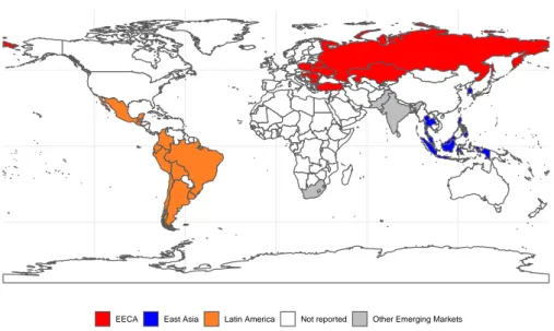
We collect quarterly frequency data for 31 emerging markets over the period 1995Q4- 2017Q1. In Figure 1 we display the regional composition of our sample.1
Figure 1: Countries Sample
EECA East Asia Latin America Not reported Other Emerging Markets
2.1 Sudden stops
Our definition of sudden stop follows step-by-step the algorithm developed byForbes and Warnock[2012] and
matches our theoretical understanding of sudden stops: a large drop in foreign capital inflows that persists over a prolonged period of time. For all the countries in our sample, we obtain total gross inflows in a quarter by summing up the total liabilities flows in the Financial Account i.e. Foreign Direct Investments (FDIs), portfolio investments and other investments liabilities. Data on inflows are retrieved from the International Financial Statistics (IFS) database of the IMF.
In practice, let us define Ci ,t as the total inflows for a country i in a quarter t . We calculate the cumulative
sum of yearly inflows for each country as Ci ,tsum=P3
s=0Ci ,t −sand calculate the yearly growth rate∆Ci ,tsum= Ci ,tsum−
Csum
i ,t −4to remove seasonality issues. We then compute the rolling mean and standard deviation for∆Ci tsum over
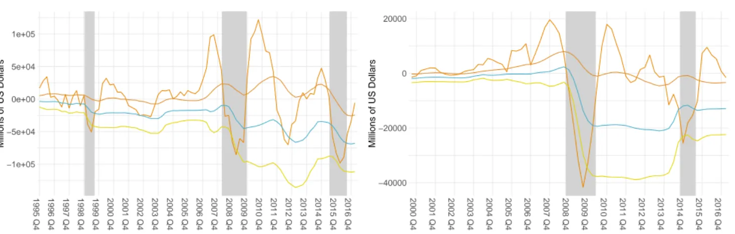
a period of 5 years. We identify a sudden stop when∆Ci ,tsum drops by more than 2 standard deviations below its rolling mean. The episode, however, begins when the drop is greater than one standard deviation from the mean.23Figure 2 shows a graphical example of the algorithm.
1For a full list, see Table 8 in the appendix.
2We exclude episodes that last only one quarter and collapse adjacent sudden stops into the same episode if the gap among the end of the former and
the start of the latter is equal or lower than two quarters.
Figure 2: Examples of Sudden Stops Identification (a) Brazil −1e+05 −5e+04 0e+00 5e+04 1e+05 1995 Q4 1996 Q4 1997 Q4 1998 Q4 1999 Q4 2000 Q4 2001 Q4 2002 Q4 2003 Q4 2004 Q4 2005 Q4 2006 Q4 2007 Q4 2008 Q4 2009 Q4 2010 Q4 2011 Q4 2012 Q4 2013 Q4 2014 Q4 2015 Q4 2016 Q4 Millions of US Dollars (b) Ukraine −40000 −20000 0 20000 2000 Q4 2001 Q4 2002 Q4 2003 Q4 2004 Q4 2005 Q4 2006 Q4 2007 Q4 2008 Q4 2009 Q4 2010 Q4 2011 Q4 2012 Q4 2013 Q4 2014 Q4 2015 Q4 2016 Q4 Millions of US Dollars
Note: The figure shows the algorithm proposed byForbes and Warnock[2012] for the identification of sudden stops applied to our sample. A sudden stop begins when the y-o-y gross capital inflows (dark orange line) go below their rolling mean minus one standard deviation (light blue line) conditional on crossing the rolling mean minus two standard deviations (yellow line). The episode ends when y-o-y gross inflows come back above their rolling mean minus one standard deviation. The duration is highlighted by the grey shaded area.
We identify a total of 75 sudden stops (SSi ,t).4Figure 3a shows the number of countries experiencing a sudden
stop throughout the sample period. Clusters of sudden stops generally correspond to very well known macroe-conomic and financial events e.g. the East Asian crisis, the Global Financial Crisis (GFC) and the turbulence following the normalization of US monetary policy in the post-GFC period. Panel 3b, instead, highlights the characteristic of regional contagion in sudden stops: episodes tend to occur temporally closely in the same EM region.
Figure 3: Number of Sudden Stops over time
(a) Aggregate 0 2 4 6 8 1995 Q4 1996 Q4 1997 Q4 1998 Q4 1999 Q4 2000 Q4 2001 Q4 2002 Q4 2003 Q4 2004 Q4 2005 Q4 2006 Q4 2007 Q4 2008 Q4 2009 Q4 2010 Q4 2011 Q4 2012 Q4 2013 Q4 2014 Q4 2015 Q4 2016 Q4 Number of Ev ents (b) By Region 0 2 4 6 8 1995 Q4 1996 Q4 1997 Q4 1998 Q4 1999 Q4 2000 Q4 2001 Q4 2002 Q4 2003 Q4 2004 Q4 2005 Q4 2006 Q4 2007 Q4 2008 Q4 2009 Q4 2010 Q4 2011 Q4 2012 Q4 2013 Q4 2014 Q4 2015 Q4 2016 Q4 Number of Ev ents
Emerging Asia Emerging Europe Latin America Other Emerging Markets
episode. We use this longer definition of duration in the robustness part.
2.2 Explanatory Variables
We test an extensive set of indicators that includes both domestic and global factors, drawing from the literature on financial crises.5Starting from domestic factors, we evaluate the significance of real economic developments through growth and inflation. A low growth pre-crisis can spark some doubts on the willingness of the monetary authority to raise the policy rate in response to capital outflows and fuel a self-fulfilling speculative attack [
Ob-stfeld,1986]. Similarly, low growth may undermine fiscal solvency and spread fear of repayment across external
creditors. On the other hand, high growth can create problems in the financial sector of the economy through higher risk appetite, credit growth and the formation of asset bubbles (Gourinchas and Obstfeld[2012]).
Like-wise, periods of high inflation often signal excesses on the monetary and fiscal side, but low inflation may be dangerous as well, especially for small open economies, warning of a surge in inflows and a rapidly appreciat-ing currency. The pre-2008 EWSs literature has also highlighted the importance of external sector variables, in particular real exchange rate, international reserves and current account [Bussière and Fratzscher,2006]. Other
variables belonging to this category are the trade balance, as an alternative to the current account, and short-term liabilities, that expose countries to roll-over risk and have been cited as a key factor in the Asian meltdown of 1997-98 [Rodrik et al.,1999]. We also test the significance of bilateral trade contagion: crisis countries "infect"
their main trading partners through import compression and higher competitiveness of their products, given the real devaluation that often follows a sudden stop.6 The interplay between domestic banking problems and capital flows [Kaminsky and Reinhart,1999] is captured through measures of credit developments. Lastly, we
include both trade and capital openness measures for which we do not have a clear prior on the direction of the impact.
Moving to global factors, after the influential paper byRey[2015], the VIX has become the standard proxy for
the Global Financial Cycle.7 Another measure that we use to capture global risk is the TED spread.8 Inter alia,
Fratzscher[2012] finds an important negative relationship between liquidity risk and flows to EMEs in the
pre-2008 period. We also try different rates: the 10-years global and US bonds yield and the 3-months T-bills rate. Historically, there has been a strong negative correlation between gross capital inflows to EME and interest rates
5See for exampleFrankel and Saravelos[2012].
6For a detailed review of contagion variables and their transmission mechanism, seeCaramazza et al.[2000]. In theory, trade contagion can also occur
through competition in third markets, but capturing this channel properly is extremely difficult as it would require bilateral trade data dis-aggregated at the product level: two countries may have a common trading partner, but sell two entirely different and unrelated products.
7While many papers confirm the central role this variable plays in outflows from EME (Forbes and Warnock[2012],Comelli[2015],Eichengreen and
Gupta[2016]), its importance has been recently challenged (Cerutti et al.[2017] andAvdjiev et al.[2017]).
8The spread rises when either the inter-bank market is fragmented and banks prefer to sit idle on their excess liquidity or when the demand for safe
in the financial centres [Reinhart,2018]. High money growth in centre countries can flag rising vulnerabilities
in the banking and financial sector and be positively correlated with sudden stops. That said, it can also portray the monetary and debt management stance in AE and thus, be negatively correlated. Other interesting variables are measures of global economic activity. Broner et al.[2013] find that capital flows both in EME and AE are
procyclical: they flow out in good times and flow in during bad times. We test both global growth and inflation as proxies.
2.3 Data Transformation
Different variables previously listed are non stationary. To avoid cases of spurious relationship, we need to re-move their deterministic and/or stochastic trend. This process is carried out in two distinct manners: by way of a one-sided HP filter or through the calculation of growth rates. When dealing with EWSs, one must also be careful to not include future information in the out-of-sample forecasting exercise: the one-sided filter ensures the ful-fillment of this criterion. We compute absolute deviations from the HP trend (gaps) using two different values for
λ, the smoothing parameter. In one case we set λ = 1600 while in the other λ = 400000, allowing for a more slowly
updating trend and more ample fluctuations.9Equivalently, growth rates are also calculated on two frequencies: year-on-year and the four-years horizon. Without imposing any a priori constraint on the model, we keep the best performers in the final specification of the EWS. We report all variables with the respective transformations tested in Table 1.10
9Some financial variables like banking credit to the private sector might exhibit a lower frequency cycle [Drehmann et al.,2012]. In the same way, real
exchange rates deviations might be quite persistent, especially for countries adopting a fixed exchange rate regime [Beutel et al.,2018].
10To further verify that there is a true relationship between the underlying variables and the probability of a sudden stop, in other words that our results
do not hinge on the de-trending approach chosen, we substitute the variable of interest with its alternative transformation in the robustness part of the paper.
Table 1: List of variables tested
Variable Level Year-on-year growth rate Four-years growth rate HP Filter (λ = 1600) HP Filter (λ = 400000) Global Factors:
VIX x
TED Spread x
Global 10-years nominal rate x US 10-years nominal rate x US Federal Funds Rate x
Global Real GDP x x
Global CPI x x
Global Liquidity (M2) x x
Domestic Factors:
Real GDP x x x x
Current Account over GDP (%) x
Private Credit over GDP (%) x x x x
Real Exchange Rate x x x x
International Reserves over GDP (%) x
International Reserves x x
Short-term Liabilities to BIS Banks over GDP (%) x Reserves (% of ST Liabilities) x
CPI x x
Trade Balance over GDP (%) x Trade Openess (% GDP) x
Trade Contagion x
Capital Controls Measures x Macroprudential Measures (Loan-to-Value) - IMaPP x
Note: The table reports the main indicators tested in the construction of the Early Warning. The first column shows the description of the variable; the ”Level” column indicates whether the level of the variable has been tested; the ”Year-on-year growth rate” and ”Four-years growth rate’ columns indicate
whether, respectively, yearly and four years growth rates of the variable have been tested; the ”HP Filter (λ = 1600)” and ”HP Filter (λ = 400000)” indicate
whether percentage deviations from Hodrick–Prescott trends of the variable have been tested: “short” (“long”) Hodrick–Prescott trend is computed with
the smoothing parameterλ set to 1600 (400000).
Finally, to normalise the scale of the regressors and address the problem of large outliers, we convert all vari-ables in country specific percentiles [Berg et al.,2005]: the fundamental assumption behind this normalisation is
that it is not the value of the indicators per se that matters, but rather their position with respect to their historical distribution.
3 Methodology
3.1 Dependent Variable
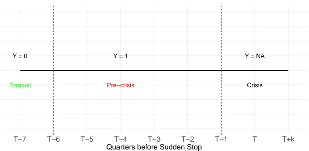
We focus on forecasting a sudden stop in gross inflows within a time window before the happening of the event. This kind of flexibility is usually allowed in EWSs given the intrinsic difficulty in predicting with precision the timing of a crisis.11We set this time interval to 6 quarters before the realization of the sudden stop: nevertheless, we leave out a gap of one quarter between the window and the start of the crisis so that the dependent variable is equal to 1 between 2 and 6 quarters before the actual sudden stop (“pre-crisis period)”. The reasons for this last choice are two. First, we want to mitigate endogeneity concerns. Endogeneity could arise because the behaviour of our indicators in the quarter preceding the sudden stop is driven by expectations of an upcoming crisis. In the same way, the actual time of start of the sudden stop may precede our definition because of measurement errors. This would lead us to include a crisis period in our dependent variable, thus introducing a bias in our estimates. Second, a useful Early Warning must leave enough time for policy action after a signal is issued and a single quarter may not be sufficient. We drop the start of the sudden stop and the quarters of its duration before the estimation. If not removed, these observations would generate a post-crisis bias for variables that during the crisis magnify the movement pre-crisis.12 Figure 4 shows in a stylized way the definition of our dependent variable.
Figure 4: Dependent Variable Definition
Y = 1 Y = NA
Y = 0
Pre−crisis Crisis
Tranquil
T−7 T−6 T−5 T−4 T−3 T−2 T−1 T T+k
Quarters before Sudden Stop
Note: T and K indicate, respectively, the start of the sudden stop and the duration of each individual episode.
11While the buid-up of domestic vulnerabilities and the worsening of global macroeconomic conditions is observable (the “causa remota”), the “causa
proxima” that drives foreign investors away is random and not foreseeable.
3.2 Estimation Strategy
We employ a standard Logit model to estimate the model and compute in and out-of-sample probabilities. The non-linear properties of this kind of models is ideal for our classification problem. Most probably, indeed, the effect of the relevant indicators is not linear, but follows an S-shape.
While scholars have recently applied new techniques that exploit Machine Learning (ML) algorithms to solve these classification problems, clear-cut evidence on the best performing method does not exist.13 Interpretabil-ity is also a concern. Logit models provide a clear ranking of the predictors, enhancing the understanding of crises by policymakers. This is particularly important in the context of our study since we include both domestic and global variables and has deep implications. If local factors are found to matter, the usefulness of predicting a crisis rises: policymakers receiving the signal, indeed, have the possibility to target the fundamentals responsible for the rise in probability and lower the overall risk, possibily avoiding the materiliazation of the event. On the other hand, if capital outflows are only determined by policy decisions in the centre countries, even if a crisis is predicted well in advance, the scope for reaction is heavily limited. Compared to parametric methods, causal inference in ML is not clear.14
For the estimation, we pool observations across time and countries.15The final specification is:
P (Yi ,t= 1) = F (Xi ,tβ) =
eXi ,tβ
1 + eXi ,tβ (1)
3.3 Evaluation
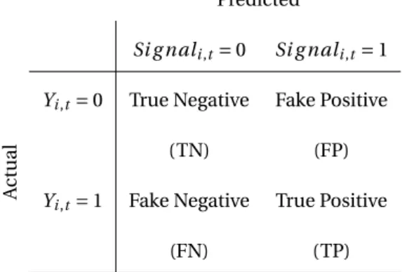
To classify predicted probabilities into binary signals, we need to impose a threshold: if the predicted probability crosses this value, a signal is sent, otherwise not. The signals are then compared to the actual value and the performance of the model is evaluated. This choice implies a trade-off between Type 1 error i.e. missing a crisis and Type 2 error i.e. issuing a fake alarm. The lower the threshold, the more fake alarms are issued and the other way around. The four possible outcomes of a classification problem are shown in table 2.
13Beutel et al.[2018] andComelli[2014], for banking and currency crises respectively, find that standard Logit models outperform different ML
algo-rithms in the out-of-sample forecasting, whileHolopainen and Sarlin[2016] find exactly the opposite for banking crises.
14Although some steps have been recently taken in this direction, see for exampleSuss and Treitel[2019].
Table 2: Example of Confusion Matrix Predicted Si g nali ,t= 0 Si g nali ,t= 1 A c tual
Yi ,t= 0 True Negative Fake Positive
(TN) (FP)
Yi ,t= 1 Fake Negative True Positive
(FN) (TP)
It follows that for any fixed thresholdτ the loss function of a policy-maker can be written as:
L(θ,τ) = θ F N (τ)
F N (τ) + T P+ (1 − θ)
F P (τ)
F P (τ) + T N (2)
whereθ indicates the preference for Type 2 errors as compared to Type 1 errors. A θ higher than 0.5 indicates that missed crises weigh more than fake alarms on the policy-maker loss function. It has become standard to set the optimal thresholdτ∗to maximize the relative usefulness of a model:
Ur(θ,τ) = 1 −
L(θ,τ)
mi n(θ,1 − θ) (3)
This function compares the usefulness of an EWS with a naive rule. The rationale is that policy-makers can always realize a loss of mi n(θ,1−θ) disregarding any model by always or never signalling an alarm . If θ is smaller than 0.5, policy-makers give more weight to Type 2 errors: the benchmark is obtained by ignoring the EWS, which amounts to never having any signals issued so that TP = FP = 0. The resulting loss according to equation 2 isθ. If
θ exceeds 0.5, they give more weight to Type 1 errors. The benchmark is to assume there is always a sudden stop:
in this case a signal is always issued so that FN = TN = 0. The resulting loss is 1 − θ. When θ = 0.5, indipendently from the naive rule chosen, the loss is the same and equal to 0.5. From equation 3, an EWS is the more useful, the lower the loss it generates with respect to a completely uninformed decision. In this context, not only this function is appropriate to find an optimal threshold, but also furnishes a natural and simple way to evaluate and compare the overall performance of different models.16
16The parameterθ is unobservable and must be set exogenously. For our benchmark forecasts, we choose a standard value of θ = 0.5 that indicates a
3.4 Forecasting Procedure
We must spend some words on the out-of-sample forecasting procedure. Our analysis is conducted in a quasi real-time manner and the evaluation period goes from 2006Q1 to 2017Q1, a time span that corresponds to half of our original sample. Hereafter we list all the steps of the exercise:
(i) At each quarter t of the evaluation period, we divide between a training sample that goes from 1995Q4 (the beginning of the original sample) to quarter t − 1 and a test sample composed exclusively by quarter t. The indicators are transformed into country-specific percentiles for the training sample.
(ii) We estimate the model on the training sample and save the optimal threshold i.e. the one that maximizes the in-sample relative usefulness function.
(iii) Re-calculating the percentiles, we compute the pre-crisis probability for quarter t . We store it together with the respective optimal threshold and recursively repeat these three steps for every quarter t until 2017Q1.17 (iv) Ex post, we compare the collected probabilities with the respective threshold, count the number of missed
signals and fake alarms and evaluate the model.
The whole procedure is designed so as to mimic as closely as possible the information available to policy-makers in each quarter and at the same time, we are careful to not introduce future information in the forecasts produced and bias the results in favor of our model.1819
4 Results
4.1 Determinants of Sudden Stops
Table 3 shows the result for our preferred specification considering the whole sample period (1995-2017): we include in our benchmark model only indicators that are significant at the 5% level and have the expected sign. For variables that are highly collinear e.g. alternative transformations or overlapping definitions, we include the
17This passage is needed to have the position of the new observation with respect to the historical distribution.
18A pitfall of this exercise is the forward-looking nature of the dependent variable Y
i ,t. This tricky point can be better explained with an example.
Imagine we are in 2005Q4 and want to estimate the pre-crisis probability for the first quarter of the out-of-sample exercise, 2006Q1. The training model will be estimated with data from 1995Q4 to 2005Q4. If between 2006Q1 and 2007Q2 a sudden stop occurs, the dependent variable in the training sample will identify some pre-crisis observations with value 1, hence incorporating future knowledge in the model. To correct, at each recursive update of the training sample, we set the last 6 quarters observations equal to 0 before estimating the model. This correction is consistent with the noise in the information set of the policy-maker: they do not know whether the build-up observed in other countries will materialize in a sudden stop.
one that maximizes the goodness of fit as measured by the relative usefulness function. Robustness checks and alternative variables are reported in appendix C.1.1.
Table 3: Full Sample Logit
Dependent variable:
Pre-crisis
TED Spread 1.504∗∗∗
(0.236)
Global Liquidity Growth −1.258∗∗∗
(0.264)
Credit-Gap 1.059∗∗∗
(0.245)
RER-Gap −1.912∗∗∗
(0.251)
ST Liabilities to BIS Banks/GDP 0.725∗∗∗
(0.237)
CA/GDP −1.108∗∗∗
(0.240)
Trade Contagion 0.700∗∗∗
(0.170)
Controls on Capital Inflow −0.432∗∗
(0.198)
Constant −1.281∗∗∗
(0.291)
Observations 1,753
Log Likelihood −716.762
Akaike Inf. Crit. 1,451.524
Note: The sample consists of 31 Emerging Markets over the period 1995Q1-2017Q1. Robust standard errors in parentheses. Global liquidity growth is
calculated on the four-years horizon. RER-Gap and Credit-Gap are deviations from Hodrick-Prescott trends withλ = 1600. Controls on capital inflows are
fromFernández et al.[2015]. * Statistical significance at 10% level. ** Statistical significance at 5% level. *** Statistical significance at 1% level.
Table 4 reports the relative goodness-of-fit statistics. The model calls correctly 62.6 % of the pre-crisis quarters with only 20% of fake alarms. The conditional probability of a crisis given a signal from the model is 40%, double the unconditional probability of experiencing a crisis (23%). Similarly, compared to a completely uninformed decision (see section 3.3), the model generates a relative usefulness for a policymaker of roughly 40%.
Table 4: In-sample Performance
Si ,t= 0 Si ,t= 1
Yi ,t= 0 1108 311
Yi ,t= 1 125 209
True Positives rate: 62.6% True Negatives rate: 78.1%
Prob. pre-crisis given a signal: 40.2% Prob. pre-crisis given no signal: 10.1% Relative Usefulness: 40.7%
Note: The table reports the results for the in-sample performance of the benchmark logit. The forecast horizon is 1-6 quarters ahead and the preference
parameterθ is equal to 0.5. The evaluation is carried out through the above measures: True Positives rate = TP/(TP+FN), True Negatives rate = TN/(TN+FP),
Prob. sudden stop given a signal = TP/(TP+FP), Prob. sudden stop given no signal = FN/(FN+TN) and Relative Usefulness Ur(see formula 3-4). Threshold
optimized in-sample to maximize the relative usefulness and equal to 23.4%.
Are crises the byproduct of domestic shortcomings or are emerging markets solely at the mercy of policy decisions and economic conditions in the global financial centres? Since our model is non-linear, we cannot directly interpret its coefficients. To calculate marginal effects and understand the relative importance of each indicator, we have, instead, to set precise values for all variables. Figure 5 shows marginal effects under a specific scenario i.e. moving the variable of interest from its tranquil time to its pre-crisis average, while other indicators are kept equal to their tranquil time average.
Figure 5: Marginal Effects Covariates
Controls on Capital Inflows Short−Term Debt/GDP Trade Contagion CA/GDP Credit−Gap Global Liquidity Growth TED Spread RER−Gap
0 1 2
Domestic Global
Note: Marginal effects calculated increasing the value of each variable individually from its tranquil time average to its pre-crisis average and keeping other covariates at their tranquil time average. Coefficients retrieved from the benchmark specification. X-axis in percentage points.
Exchange rate overvaluation and rise in the TED spread have the strongest impact, increasing the probability of a sudden stop by more than 2.5 percentage points (pp). Global liquidity tightening, credit booms and current account deficits compose a second group and have a smaller impact (1.5 pp). At the end of the spectrum follow trade contagion and short-term debt (1 pp) and last, controls on capital inflows (less than 0.5 pp). Even though
these effects may appear relatively small, one must bear in mind different points: first, the pre-crisis period is long, starting a year and a half prior to the crisis, thus influencing the value of the pre-crisis average. Second, the reference point matters: while to isolate the effects we have kept all other indicators to their tranquil aver-age, in practice a rise in the TED spread might have a much larger effect, for example, when also the current account deficit is large. All in all, we do not find strong evidence of predominance by neither of the two group of factors: this is suggestive that policymakers have at least some leeway to act targeting weak fundamentals when confronted with a newly issued signal.
4.2 Out-of-Sample Performance and Forecast Horizon
The paper byBerg and Patillo[1999] pointed to a large divergence between the in and out-of-sample
perfor-mance for EWSs. Since then it has become standard to evaluate the predictive power of these models on the base of their out-of-sample performance. The framework developed in section 3.4 allows us to do so in a quasi-real time manner i.e. having the same information set of the policymaker at the time of the prediction and without introducing future knowledge in the model.20 The results of the out-of-sample estimation are reported in Table 5.
Table 5: Out-of-sample Performance
Si ,t= 0 Si ,t= 1
Yi ,t= 0 648 117
Yi ,t= 1 129 116
True Positives rate: 47.4% True Negatives rate: 84.7%
Prob. sudden stop given a signal: 50% Prob. sudden stop given no signal: 16% Relative Usefulness: 32%
Note: The table reports the results for the quasi real-time out-of-sample performance of the benchmark logit. The forecast horizon is defined in section ??
and the preference parameterθ is equal to 0.5. The evaluation is carried out through the above measures: True Positives rate = TP/(TP+FN), True Negatives
rate = TN/(TN+FP), Prob. sudden stop given a signal = TP/(TP+FP), Prob. sudden stop given no signal = FN/(FN+TN) and Relative Usefulness Ur(see
formula 3-4).
The EWS predicts almost 50% of the pre-crisis episodes while sending relatively few alarms, about 15% of the total tranquil quarters. This means every time a signal is sent, there is a 50% probability of a correct call, a percentage higher than its in-sample counterpart. Thus, the uncertainty involved by our model in the out-of-sample predictions is limited. Overall, the EWS would result in a 32% gain compared to a completely uninformed decision for a policy-maker with balanced preferences between Type 1 and Type 2 errors.
The result is robust to the choice of a different time horizon as shown in Table 6. The relative usefulness statistics always remains around 30% and reaches its maximum for our 6 quarters benchmark, validating ex post our choice. Moving to the 8 quarters specification, the number of correctly identified pre-crisis periods increases (TP Rate), but also does the amount of fake alarms (1-TN Rate). This is suggestive that for policymakers with a greater value forθ the choice of a longer horizon span would be preferable.
Table 6: Different forecast horizons out-of-sample performance
Forecast Horizon TP TN FP FN TP Rate TN Rate P(Pre-crisis|Signal) P(Pre-crisis|No Signal) Ur(θ)
4 Quarters 73 719 137 81 47.4% 84% 34.8% 10.1% 31.4%
6 Quarters 116 648 117 129 47.4% 84.7% 50% 16% 32%
8 Quarters 163 538 142 163 49.4% 79.1% 53% 23.7% 28%
Note: The table reports the results for the quasi real-time out-of-sample performance of the benchmark logit changing the forecast horizon. The preference
parameterθ is equal to 0.5. The evaluation is carried out through the above measures: True Positives rate = TP/(TP+FN), True Negatives rate = TN/(TN+FP),
Prob. sudden stop given a signal = TP/(TP+FP), Prob. sudden stop given no signal = FN/(FN+TN) and Relative Usefulness Ur(see formula 3-4).
4.3 Timing
How did our model work with particular reference to the 2008 crisis? With how much certainty were the signal sent? And were they timely? In panel 6a we show the distribution of the out-of-sample predicted probabilities for the GFC episodes during the individual pre-crisis periods and we condition on the EM regional group. While for Emerging Europe the bulk of the distribution i.e. the probability of being in a pre-crisis quarter, is around 80%, for East Asia most of the individual probabilities reach only 20%. For Latin American the distribution is, instead, more uniform. For the first group of countries, the first signal was sent, on average, more than one year before the sudden stop (Figure 6b). For the second, instead, episodes were not signalled at all or just with a small advance. Latin America, as before, lies in between.
Figure 6: GFC Sudden Stops
(a) Out-of-sample probabilities
| | | | | | | | || | || | | | | | | ||| ||| | |||| | | | | | |||||||| | ||||||| ||| ||||| |||| || | | | | |||| ||| || || || | || East Asia Latin America Emerging Europe 0.0 0.2 0.4 0.6 0.8 1.0 (b) First Signal East Asia Latin America Emerging Europe 0 1 2 3 4 5
Note: Panel (a) shows the distribution of the predicted probabilities for the out-of-sample recursive exercise in the pre-crisis period of each country-specific Global Financial Crisis sudden stop. We consider Global Financial Crisis sudden stops those episodes occurring in the time window 2006Q4 - 2008Q4. Panel (b) shows for the aforementioned episodes the advance, on average, of the model in issuing a signal. X-axis indicates quarters before the sudden stop.
Domestic factors largely explain this heterogeneity of results between regional groups. East Asian countries enforced counter cyclical fiscal and monetary policy in the years that followed the regional crisis of 1997-98, approaching 2008 with large current account surpluses, a competitive and flexible exchange rate and a solid fi-nancial sector.2122EECA countries, instead, neared the GFC with extremely flawed fundamentals. Pre-2008 cap-ital inflows financed exceptionally large current account deficits with a considerable part of this foreign capcap-ital that was channeled into short-term maturities: real exchange rates appreciated steeply and there was a lending boom operated by the banking sector [Gourinchas and Obstfeld,2012]: this surge was allowed by a simultaneous
liberalization of capital markets.
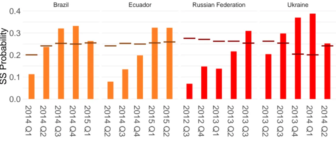
We then move to the post-GFC period and ask the same question. While sudden stops in the GFC are more or less synchronized, afterwards they are more distributed across the test period: instead of a regional aggrega-tion, we proceed on a case-by-case basis. In particular, we study the behavior of fitted probabilities before four interesting crises: Russia 2014 Q1, Ukraine 2014 Q3, Brazil 2015 Q3 and Ecuador in 2015 Q4 (Figure 7).23
21See for examplePark et al.[2013].
22South Korea and Indonesia are the countries in the group with the highest predicted probabilities. The first had sound macroeconomic fundamentals,
but a large level of short-term dollar denominated liabilities in the banking sector. The second was the last country in the region to experience a reversal of gross inflows and as such probabilities are greatly influenced by shattered global factors and regional contagion.
23We focus on these occurrences because they are associated with at least a quarter of recession throughout the sudden stop duration, while other
Figure 7: Post GFC Sudden Stops
Brazil Ecuador Russian Federation Ukraine
2014 Q1 2014 Q2 2014 Q3 2014 Q4 2015 Q1 2014 Q2 2014 Q3 2014 Q4 2015 Q1 2015 Q2 2012 Q3 2012 Q4 2013 Q1 2013 Q2 2013 Q3 2013 Q2 2013 Q3 2013 Q4 2014 Q1 2014 Q2 0.0 0.1 0.2 0.3 0.4 SS Probability
Note: Out-of-sample fitted probabilities in the pre-crisis period for four different sudden stops episodes: Brazil 2015Q3, Ecuador 2015 Q4, Russian Federation 2014 Q1 and Ukraine 2014 Q4. The thick line corresponds to the time-varying optimal threshold.
Our EWS sends a signal half a year before for Russia, the minimum allowed. For the other crises, the advance widens: Ukraine is called more than one year in advance, Brazil one year and Ecuador three quarters. Even though probabilities are much lower compared to the GFC, owing mostly to improved global conditions, is ex-tremely encouraging that all the four episodes would have been signalled with advance.24 Moreover, this result is achieved without considering important factors that analyst have linked to these crises: worsening political landscape (Ukraine and Brazil) and the occurrence of natural disasters (Ecuador). This means that even if the last two may have contributed to the drop in inflows, multiple factors exerted pressure on these countries.
4.4 Sudden Stop Impact and Fitted Probabilities
Hitherto we based the evaluation of our EWS solely on missed crises (Type 1 errors) and fake alarms (Type 2 errors), in line with the literature. The underlying assumption of such an evaluation framework is that external crises are alike episodes and produce the same effects on the economies hit. Nevertheless, it is a well-known fact that some crises are more painful than others. This owes to different factors: the magnitude of the external shock, the conditions of the domestic economy at the time and of course, the policy response that follows as well as the behaviour of domestic investors. These elements are not mutually exclusive, but rather complementary.
Therefore, when evaluating an EWS, policymakers should also be concerned about which specific events are predicted and which not. In doing so, the novelty of this paper is that we link two parts of the literature that have so far been kept separated: one is the classic EWS literature that tries to predict in advance the occurrence
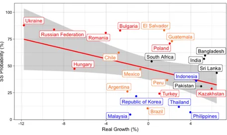
of a crisis, while the second, instead, tries to predict its incidence. Figure 8 shows the relationship between the estimated pre-crisis median probability and the median growth experienced during the episode for every country-specific sudden stop in the GFC.
Figure 8: Fitted Probabilities and Ex-Post Growth
Note: The figure shows the relationship between the median out-of-sample probability in the pre-crisis period for GFC related sudden stops and the median growth during the associated sudden stop. Red line is the regression line with 95% confidence intervals.
At a first glance, EECA countries monopolize the north-western quadrant. This means these are the countries that suffered more during the GFC sudden stops and contemporaneously those that exhibit the highest median probabilities. Further, from Figure 6b, they are also the sudden stops for which a signal was sent with large advance by our model. On the other hand, East Asian countries occupy mostly the south eastern quadrant i.e. countries that suffered less and with the lowest median probabilities. Latin American countries are, once again, highly heterogeneous. We consider two countries during the GFC, one from the EECA and the other from the East-Asian group e.g. Romania and Thailand. The first suffered from a full-fledged recession with a median quarterly contraction of 4% of GDP, while the second continued to grow at a moderate pace, around 2.5%. For the first a signal would have been sent early and with extreme certainty, while the second belongs to the group of missed crises.25
We further proceed investigating formally the issue: we pool all the out-of-sample observations together and estimate the cross-sectional relationship. Table 7 shows the regression results. We find that an increase in median
25While median growth rate during the sudden stop is a simple proxy of output impact, this measure, however, ignores that countries might have different
trend growth rates before the event: therefore, we test robustness of the relationship using a different metric. We construct this new measure as the median growth rate during the sudden stop minus the median growth rate in the preceding tranquil period: the resulting scatter plot displays a similar pattern (See Figure 11 in the appendix).
pre-crisis probability by a percentage point decreases significantly growth during the sudden stop by 0.07%. Sudden stops predicted with more certainty by our EWS are also the most destructive ones in terms of output losses, while those that are not identified (Type 1 error) or identified with relatively low probabilities are those with mild consequences for the real economy. Against this new evidence, reporting standard evaluation metrics without investigating for which sudden stops a signal would have been sent and for which not, would highly underestimate the true value of an Early Warning for policymakers.
Table 7: Predicted Probability and Sudden Stop Incidence
Dependent variable: Median Growth
Coeff. Std. error t-statistic P> |t| Pre-crisis probability −0.070 0.027 −2.54 0.02
Observations 41
Note: The sample comprises the 41 sudden stops episodes occured after 2006 Q1, the beginning of the out-of-sample period. Dependent variable is the median growth calculated over the duration of each episode. Indipendent variable is the median out-of-sample probability estimated over the whole pre-crisis period. Intercept omitted and robust standard error reported.
5 Conclusion
This paper contributes to the financial crisis literature investigating the predictability of sudden stops in emerg-ing markets. We extend the existemerg-ing literature in different ways. First, we test a large variety of domestic and global indicators and evaluate their relative importance in the materialization of sudden stops: if emerging mar-kets are only at the mercy of policy decisions in the global financial centres, the scope for intervention by domes-tic policymakers results highly limited even when a signal is issued. Second, we propose a framework to evaluate the performance of the model in quasi-real time, taking heed not to include future information in the recursive exercise. Third, we study the relationship between the probabilities estimated by our model and the output loss associated with the ensuing sudden stop.
We find a near equivalence between the marginal impact of domestic and global factors on the probability of a crisis: this result highlights the role EWSs can play not only as a surveillance, but also as a stability tool available to policymakers. We then proceeded evaluating the out-of-sample performance of the model. The recursive exercise yields encouraging results with a parsimonious specification: the pre-crisis periods correctly called are close to 50% of the total with fake alarms corresponding to less than 15%. This means that the un-certainty involved with the predictions is low: compared to the unconditional probability of being in a pre-crisis quarter (roughly 20%), the conditional probability given a signal rises to 50%. Finally, we brought forward a new argument in “defense” of EWSs. We show that there is a negative, statistically and economically significant rela-tionship between the median probability predicted for the whole pre-crisis period and median economic growth experienced during the associated sudden stop: in other words, the model works well in predicting catastrophic events and less so for rather innocuous ones.
All in all, even if the prediction of rare events like sudden stops remains a humbling task, our model would have sent reliable, timely and relevant signals. This is especially promising in view of the lengthy out-of-sample horizon chosen and the different non-economic factors that exerted pressure on emerging markets in the recent decade.
References
Iñaki Aldasoro, Claudio Borio, and Mathias Drehmann. Early Warning Indicators of Banking Crises: Expanding the Family. BIS Quarterly Review, 2018.
Lucia Alessi and Carsten Detken. ’Real Time’ Early Warning Indicators for Costly Asset Price Boom/Bust Cycles -A role for Global Liquidity. ECB Working Paper, 2009.
Lucia Alessi and Carsten Detken. Identifying excessive credit growth and leverage. Journal of Financial Stability, 2018.
Stefan Avdjiev, Leonardo Gambacorta, Linda S Goldberg, and Stefano Schiaffi. The Shifting Drivers of Global Liquidity. BIS Working Papers, 2017.
Jan Babecký, Tomáš Havránek, Jakub Matˇej ˚u, Marek Rusnák, Katerina Smidková, and Vašicek Borek. Banking , Debt , and Currency Crises Early Warning Indicators for Developed Countries. ECB Working Paper, 2012.
Suman S Basu, Roberto A Perrelli, and Weining Xin. External Crisis Prediction Using Machine Learning : Evidence from Three Decades of Crises Around the World. IMF Working Paper, 2019.
Andrew Berg and Catherine Patillo. Are Currency Crises Predictable? A Test. IMF Staff Papers, 42(2):107–138, 1999.
Andrew Berg, Eduardo Borensztein, and Catherine A. Pattillo. Assessing Early Warning Systems: How Have they Worked in Practice? Imf Staff Papers, 2005.
Johannes Beutel, Sophia List, and Gregor Von Schweinitz. An evaluation of early warning models for systemic banking crises: Does machine learning improve predictions? Bundesbank Discussion Paper, 2018.
Olivier J Blanchard, Hamid Faruqee, and Mitali Das. The Initial Impact of the Crisis on Emerging Market Coun-tries. Brookings Papers on Economic Activity, 2010.
Fernando Broner, Tatiana Didier, Aitor Erce, and Sergio L Schmukler. Gross Capital Flows: Dynamics and Crises.
Journal of Monetary Economics, 60(1):113–133, 2013.
M Bussière and M Fratzscher. Towards a new early warning system of financial crises. Journal of International
Money and Finance, 2006.
Matthieu Bussière. Balance of Payment Crises in Emerging Markets : How Early Were the "Early" Warning Sig-nals? ECB Working Paper, 2007.
Matthieu Bussière. In Defense Of Early Warning Signals. Banque de France Working Paper, 2013.
GA Calvo, A Izquierdo, and LF Mejia. On the empirics of sudden stops: the relevance of balance-sheet effects.
NBER Working Paper, 2004.
Francesco Caramazza, Luca Ricci, and Ranil Salgado. Trade and Financial Contagion in Currency Crises. IMF
Working Paper, 2000.
Luis A V Catão and Gian Maria Milesi-Ferretti. External Liabilities and Crises. Journal of International Economics, 2014.
Eugenio Cerutti, S. Claessens, and Andrew K. Rose. How Important is the Global Financial Cycle? Evidence from capital flows. BIS Working Papers, 2017.
Menzie D. Chinn and Hiro Ito. A New Measure of Financial Openness. Journal of Comparative Policy Analysis:
Research and Practice, 2008.
Fabio Comelli. Comparing parametric and non-parametric early warning systems for currency crises in emerging market economies. Review of International Economics, 2014.
Fabio Comelli. Estimation and out-of-sample Prediction of Sudden Stops: Do Regions of Emerging Markets Behave Differently from Each Other? IMF Working Paper, 2015.
Mathias Drehmann, Claudio Borio, and Kostas Tsatsaronis. Characterising the Financial Cycle: Don’t Lose Sight of the Medium Term! BIS Working Papers, 2012.
Marco Lo Duca and Tuomas A. Peltonen. Assessing systemic risks and predicting systemic events. Journal of
Banking and Finance, 2013.
B Eichengreen and P Gupta. Managing sudden stops. World Bank Policy Research Working Paper, 2016.
Barry Eichengreen, Poonam Gupta, and Oliver Masetti. Are Capital Flows Fickle? Increasingly? and Does the Answer Still Depend on Type? Asian Economic Papers, 2018. ISSN 15360083. doi: 10.1162/asep{\_}a{\_}00583.
Andrés Fernández, Michael W Klein, Alessandro Rebucci, Martin Schindler, and Martín Uribe. Capital Control Measures: A New Dataset. IMF Working Paper, 2015.
Kristin J Forbes and Francis E Warnock. Capital Flow Waves: Surges, Stops, Flight, and Retrenchment. Journal of
Jeffrey Frankel and George Saravelos. Can leading indicators assess country vulnerability ? Evidence from the 2008 – 09 global financial crisis . Journal of International Economics, 2012.
Jeffrey A. Frankel and Andrew K. Rose. Currency Crashes in Emerging Markets: an Empirical Treatment.
Interna-tional Finance Discussion Papers, 1996.
Marcel Fratzscher. Push versus pull factors and the global financial crisis. Journal of International Economics, 2012.
Pierre-Olivier Gourinchas and Maurice Obstfeld. Stories of the Twentieth Century for the Twenty-First. American
Economic Journal: Macroeconomics, 2012.
Markus Holopainen and Peter Sarlin. Toward robust early-warning models: a horse race, ensembles and model uncertainty. ECB Working Paper, 2016.
Sebnem Kalemli-Ozcan. Emerging Market Capital Flows under COVID : What to Expect Given What We Know.
IMF Research, 2020.
Graciela L. Kaminsky. Varieties of currency crises. Annals of Economics and Finance, 2003.
Graciela L. Kaminsky and Carmen M. Reinhart. The Twin Crises: The Causes of Banking and Balance-Of-Payments Problems. American Economic Review, 1999.
Andrei A. Levchenko and Paolo Mauro. Do some forms of financial flows help protect against "sudden stops"?
World Bank Economic Review, 2007.
Paolo Manasse and Nouriel Roubini. "Rules of thumb" for sovereign debt crises. Journal of International
Eco-nomics, 2009. ISSN 00221996. doi: 10.1016/j.jinteco.2008.12.002.
Paolo Manasse, Nouriel Roubini, and Axel Schimmelpfennig. Predicting Sovereign Debt Crises. IMF Working
Paper, 2003.
Maurice Obstfeld. Rational and Self-Fulfilling Balance-of-Payments Crises. NBER Working Paper, 1986.
Donghyun Park, Arief Ramayandi, and Kwanho Shin. Why Asia Fare Better during the Global Financial Crisis than during the Asian Financial Crisis ? In Responding to Financial Crisis: Lessons from Asia Then, the United
States and Europe Now. 2013.
Carmen Reinhart, Graciela Kaminsky, and Saul Lizondo. Leading Indicators of Currency Crises. Staff Papers
Carmen M. Reinhart. Financial crises: past and future. AEI Economics Working Paper, 2018.
Hélène Rey. Dilemma not Trilemma: The Global Financial Cycle and Monetary Policy Independence. NBER
Working Paper, 2015.
Dani Rodrik, Andrés Velasco, and John F Kennedy. Short Term Capital Flows. NBER Working Paper, 1999.
Andrew K. Rose and Mark M. Spiegel. Cross-Country Causes And Consequences Of The 2008 Crisis: Early Warn-ing. Global Journal of Economics, 2010.
Andrew K. Rose and Mark M. Spiegel. Cross-country causes and consequences of the crisis: An update. European
Economic Review, 2011.
Joel Suss and Henry Treitel. Predicting bank distress in the UK with machine learning. Bank of England, Working
Appendices
A Data
Table 8: Countries List
Country Region
Argentina Latin America
Bangladesh Other Emerging Markets
Belarus EECA
Bolivia (Plurinational State of ) Latin America
Brazil Latin America
Bulgaria EECA
Chile Latin America
Colombia Latin America
Ecuador Latin America
El Salvador Latin America Guatemala Latin America
Hungary EECA
India Other Emerging Markets
Indonesia East Asia
Kazakhstan EECA
Malaysia East Asia
Mexico Latin America
Pakistan Other Emerging Markets
Peru Latin America
Philippines East Asia
Poland EECA
Country Region
Romania EECA
Russian Federation EECA
South Africa Other Emerging Markets Sri Lanka Other Emerging Markets
Thailand East Asia
Turkey EECA
Ukraine EECA
Uruguay Latin America
A.1 Sudden Stops
Figure 9: Sudden Stops Identification
Argentina −30000 −20000 −10000 0 10000 20000 1995 Q4 1996 Q4 1997 Q4 1998 Q4 1999 Q4 2000 Q4 2001 Q4 2002 Q4 2003 Q4 2004 Q4 2005 Q4 2006 Q4 2007 Q4 2008 Q4 2009 Q4 2010 Q4 2011 Q4 2012 Q4 2013 Q4 2014 Q4 2015 Q4 2016 Q4 Millions of US Dollars Bangladesh −2000 0 2000 1995 Q4 1996 Q4 1997 Q4 1998 Q4 1999 Q4 2000 Q4 2001 Q4 2002 Q4 2003 Q4 2004 Q4 2005 Q4 2006 Q4 2007 Q4 2008 Q4 2009 Q4 2010 Q4 2011 Q4 2012 Q4 2013 Q4 2014 Q4 2015 Q4 2016 Q4 Millions of US Dollars Belarus −10000 −5000 0 5000 2002 Q4 2003 Q4 2004 Q4 2005 Q4 2006 Q4 2007 Q4 2008 Q4 2009 Q4 2010 Q4 2011 Q4 2012 Q4 2013 Q4 2014 Q4 2015 Q4 2016 Q4 Millions of US Dollars Bolivia −2000 0 2000 1995 Q4 1996 Q4 1997 Q4 1998 Q4 1999 Q4 2000 Q4 2001 Q4 2002 Q4 2003 Q4 2004 Q4 2005 Q4 2006 Q4 2007 Q4 2008 Q4 2009 Q4 2010 Q4 2011 Q4 2012 Q4 2013 Q4 2014 Q4 2015 Q4 2016 Q4 Millions of US Dollars Brazil −1e+05 −5e+04 0e+00 5e+04 1e+05 1995 Q4 1996 Q4 1997 Q4 1998 Q4 1999 Q4 2000 Q4 2001 Q4 2002 Q4 2003 Q4 2004 Q4 2005 Q4 2006 Q4 2007 Q4 2008 Q4 2009 Q4 2010 Q4 2011 Q4 2012 Q4 2013 Q4 2014 Q4 2015 Q4 2016 Q4 Millions of US Dollars Bulgaria −10000 0 10000 1997 Q4 1998 Q4 1999 Q4 2000 Q4 2001 Q4 2002 Q4 2003 Q4 2004 Q4 2005 Q4 2006 Q4 2007 Q4 2008 Q4 2009 Q4 2010 Q4 2011 Q4 2012 Q4 2013 Q4 2014 Q4 2015 Q4 2016 Q4 Millions of US Dollars
Chile −20000 −10000 0 10000 20000 1997 Q4 1998 Q4 1999 Q4 2000 Q4 2001 Q4 2002 Q4 2003 Q4 2004 Q4 2005 Q4 2006 Q4 2007 Q4 2008 Q4 2009 Q4 2010 Q4 2011 Q4 2012 Q4 2013 Q4 2014 Q4 2015 Q4 2016 Q4 Millions of US Dollars Colombia −10000 0 10000 2002 Q4 2003 Q4 2004 Q4 2005 Q4 2006 Q4 2007 Q4 2008 Q4 2009 Q4 2010 Q4 2011 Q4 2012 Q4 2013 Q4 2014 Q4 2015 Q4 2016 Q4 Millions of US Dollars Ecuador −5000 0 5000 1998 Q4 1999 Q4 2000 Q4 2001 Q4 2002 Q4 2003 Q4 2004 Q4 2005 Q4 2006 Q4 2007 Q4 2008 Q4 2009 Q4 2010 Q4 2011 Q4 2012 Q4 2013 Q4 2014 Q4 2015 Q4 2016 Q4 Millions of US Dollars El Salvador −2000 −1000 0 1000 2004 Q4 2005 Q4 2006 Q4 2007 Q4 2008 Q4 2009 Q4 2010 Q4 2011 Q4 2012 Q4 2013 Q4 2014 Q4 2015 Q4 2016 Q4 Millions of US Dollars Guatemala −3000 −2000 −1000 0 1000 2000 1995 Q4 1996 Q4 1997 Q4 1998 Q4 1999 Q4 2000 Q4 2001 Q4 2002 Q4 2003 Q4 2004 Q4 2005 Q4 2006 Q4 2007 Q4 2008 Q4 2009 Q4 2010 Q4 2011 Q4 2012 Q4 2013 Q4 2014 Q4 2015 Q4 2016 Q4 Millions of US Dollars Hungary −1e+05 −5e+04 0e+00 5e+04 1e+05 1999 Q4 2000 Q4 2001 Q4 2002 Q4 2003 Q4 2004 Q4 2005 Q4 2006 Q4 2007 Q4 2008 Q4 2009 Q4 2010 Q4 2011 Q4 2012 Q4 2013 Q4 2014 Q4 2015 Q4 2016 Q4 Millions of US Dollars
India −80000 −40000 0 40000 1997 Q4 1998 Q4 1999 Q4 2000 Q4 2001 Q4 2002 Q4 2003 Q4 2004 Q4 2005 Q4 2006 Q4 2007 Q4 2008 Q4 2009 Q4 2010 Q4 2011 Q4 2012 Q4 2013 Q4 2014 Q4 2015 Q4 2016 Q4 Millions of US Dollars Indonesia −20000 0 20000 1995 Q4 1996 Q4 1997 Q4 1998 Q4 1999 Q4 2000 Q4 2001 Q4 2002 Q4 2003 Q4 2004 Q4 2005 Q4 2006 Q4 2007 Q4 2008 Q4 2009 Q4 2010 Q4 2011 Q4 2012 Q4 2013 Q4 2014 Q4 2015 Q4 2016 Q4 Millions of US Dollars Kazakhstan −30000 −20000 −10000 0 10000 20000 2001 Q4 2002 Q4 2003 Q4 2004 Q4 2005 Q4 2006 Q4 2007 Q4 2008 Q4 2009 Q4 2010 Q4 2011 Q4 2012 Q4 2013 Q4 2014 Q4 2015 Q4 2016 Q4 Millions of US Dollars Malaysia −40000 0 40000 2007 Q4 2008 Q4 2009 Q4 2010 Q4 2011 Q4 2012 Q4 2013 Q4 2014 Q4 2015 Q4 2016 Q4 Millions of US Dollars Mexico −50000 −25000 0 25000 1995 Q4 1996 Q4 1997 Q4 1998 Q4 1999 Q4 2000 Q4 2001 Q4 2002 Q4 2003 Q4 2004 Q4 2005 Q4 2006 Q4 2007 Q4 2008 Q4 2009 Q4 2010 Q4 2011 Q4 2012 Q4 2013 Q4 2014 Q4 2015 Q4 2016 Q4 Millions of US Dollars Pakistan −4000 0 4000 1995 Q4 1996 Q4 1997 Q4 1998 Q4 1999 Q4 2000 Q4 2001 Q4 2002 Q4 2003 Q4 2004 Q4 2005 Q4 2006 Q4 2007 Q4 2008 Q4 2009 Q4 2010 Q4 2011 Q4 2012 Q4 2013 Q4 2014 Q4 2015 Q4 2016 Q4 Millions of US Dollars
Peru −15000 −10000 −5000 0 5000 10000 1999 Q4 2000 Q4 2001 Q4 2002 Q4 2003 Q4 2004 Q4 2005 Q4 2006 Q4 2007 Q4 2008 Q4 2009 Q4 2010 Q4 2011 Q4 2012 Q4 2013 Q4 2014 Q4 2015 Q4 2016 Q4 Millions of US Dollars Philippines −20000 −10000 0 10000 1995 Q4 1996 Q4 1997 Q4 1998 Q4 1999 Q4 2000 Q4 2001 Q4 2002 Q4 2003 Q4 2004 Q4 2005 Q4 2006 Q4 2007 Q4 2008 Q4 2009 Q4 2010 Q4 2011 Q4 2012 Q4 2013 Q4 2014 Q4 2015 Q4 2016 Q4 Millions of US Dollars Poland −75000 −50000 −25000 0 25000 2006 Q4 2007 Q4 2008 Q4 2009 Q4 2010 Q4 2011 Q4 2012 Q4 2013 Q4 2014 Q4 2015 Q4 2016 Q4 Millions of US Dollars Republic of Korea −1e+05 −5e+04 0e+00 5e+04 1e+05 1995 Q4 1996 Q4 1997 Q4 1998 Q4 1999 Q4 2000 Q4 2001 Q4 2002 Q4 2003 Q4 2004 Q4 2005 Q4 2006 Q4 2007 Q4 2008 Q4 2009 Q4 2010 Q4 2011 Q4 2012 Q4 2013 Q4 2014 Q4 2015 Q4 2016 Q4 Millions of US Dollars Romania −20000 −10000 0 10000 1997 Q4 1998 Q4 1999 Q4 2000 Q4 2001 Q4 2002 Q4 2003 Q4 2004 Q4 2005 Q4 2006 Q4 2007 Q4 2008 Q4 2009 Q4 2010 Q4 2011 Q4 2012 Q4 2013 Q4 2014 Q4 2015 Q4 2016 Q4 Millions of US Dollars Russian Federation −2e+05 −1e+05 0e+00 1e+05 2000 Q4 2001 Q4 2002 Q4 2003 Q4 2004 Q4 2005 Q4 2006 Q4 2007 Q4 2008 Q4 2009 Q4 2010 Q4 2011 Q4 2012 Q4 2013 Q4 2014 Q4 2015 Q4 2016 Q4 Millions of US Dollars
South Africa −30000 −20000 −10000 0 10000 20000 1995 Q4 1996 Q4 1997 Q4 1998 Q4 1999 Q4 2000 Q4 2001 Q4 2002 Q4 2003 Q4 2004 Q4 2005 Q4 2006 Q4 2007 Q4 2008 Q4 2009 Q4 2010 Q4 2011 Q4 2012 Q4 2013 Q4 2014 Q4 2015 Q4 2016 Q4 Millions of US Dollars Sri Lanka −2000 0 2000 2000 Q4 2001 Q4 2002 Q4 2003 Q4 2004 Q4 2005 Q4 2006 Q4 2007 Q4 2008 Q4 2009 Q4 2010 Q4 2011 Q4 2012 Q4 2013 Q4 2014 Q4 2015 Q4 2016 Q4 Millions of US Dollars Thailand −40000 −20000 0 20000 1995 Q4 1996 Q4 1997 Q4 1998 Q4 1999 Q4 2000 Q4 2001 Q4 2002 Q4 2003 Q4 2004 Q4 2005 Q4 2006 Q4 2007 Q4 2008 Q4 2009 Q4 2010 Q4 2011 Q4 2012 Q4 2013 Q4 2014 Q4 2015 Q4 2016 Q4 Millions of US Dollars Turkey −50000 0 50000 1995 Q4 1996 Q4 1997 Q4 1998 Q4 1999 Q4 2000 Q4 2001 Q4 2002 Q4 2003 Q4 2004 Q4 2005 Q4 2006 Q4 2007 Q4 2008 Q4 2009 Q4 2010 Q4 2011 Q4 2012 Q4 2013 Q4 2014 Q4 2015 Q4 2016 Q4 Millions of US Dollars Ukraine −40000 −20000 0 20000 2000 Q4 2001 Q4 2002 Q4 2003 Q4 2004 Q4 2005 Q4 2006 Q4 2007 Q4 2008 Q4 2009 Q4 2010 Q4 2011 Q4 2012 Q4 2013 Q4 2014 Q4 2015 Q4 2016 Q4 Millions of US Dollars Uruguay −5000 0 5000 2006 Q4 2007 Q4 2008 Q4 2009 Q4 2010 Q4 2011 Q4 2012 Q4 2013 Q4 2014 Q4 2015 Q4 2016 Q4 Millions of US Dollars
Venezuela −10000 0 10000 2000 Q4 2001 Q4 2002 Q4 2003 Q4 2004 Q4 2005 Q4 2006 Q4 2007 Q4 2008 Q4 2009 Q4 2010 Q4 2011 Q4 2012 Q4 2013 Q4 2014 Q4 2015 Q4 2016 Q4 Millions of US Dollars
Note: The figure shows the algorithm proposed byForbes and Warnock[2012] for the identification of sudden stops applied to our sample. A sudden stop begins when the y-o-y gross capital inflows (dark orange line) go below their rolling mean minus one standard deviation (light blue line) conditional on crossing the rolling mean minus two standard deviations (yellow line). The episode ends when y-o-y gross inflows come back above their rolling mean minus one standard deviation. The duration is highlighted by the grey shaded area.
Table 9: List of Sudden Stops
Country Quarter Duration (in quarters)
Argentina 1998 Q4 4 Argentina 2000 Q4 7 Argentina 2008 Q2 7 Bangladesh 2005 Q4 2 Bangladesh 2009 Q2 3 Bangladesh 2011 Q1 4 Belarus 2008 Q4 4 Belarus 2012 Q1 4
Bolivia (Plurinational State of ) 1999 Q2 9 Bolivia (Plurinational State of ) 2006 Q3 4 Bolivia (Plurinational State of ) 2014 Q3 4
Brazil 1999 Q1 2 Brazil 2008 Q2 6 Brazil 2015 Q3 4 Bulgaria 2008 Q4 5 Bulgaria 2015 Q4 2 Chile 2000 Q2 3 Chile 2009 Q1 3 Chile 2013 Q3 3 Colombia 2015 Q2 6 Ecuador 1999 Q2 9 Ecuador 2015 Q4 3 El Salvador 2004 Q3 2 El Salvador 2009 Q1 4 Guatemala 1999 Q4 8 Guatemala 2008 Q4 4
Country Quarter Duration (in quarters) Hungary 2002 Q2 2 Hungary 2009 Q1 5 India 2008 Q3 5 India 2015 Q4 4 Indonesia 1997 Q4 4 Indonesia 2006 Q4 2 Indonesia 2009 Q1 3 Indonesia 2011 Q4 3 Indonesia 2015 Q3 4 Kazakhstan 2007 Q4 5 Kazakhstan 2014 Q2 8 Malaysia 2008 Q3 4 Malaysia 2014 Q4 4 Mexico 2006 Q4 3 Mexico 2008 Q4 4 Mexico 2014 Q4 5 Pakistan 1998 Q3 4 Pakistan 2008 Q2 5 Peru 2008 Q4 4 Peru 2013 Q4 3 Philippines 1997 Q3 5 Philippines 2008 Q1 5 Poland 2008 Q4 4 Republic of Korea 1997 Q4 5 Republic of Korea 2008 Q2 5 Republic of Korea 2015 Q3 4 Romania 2008 Q3 7 Russian Federation 2008 Q4 4
Country Quarter Duration (in quarters) Russian Federation 2014 Q1 6 South Africa 1998 Q3 4 South Africa 2000 Q3 3 South Africa 2008 Q3 4 South Africa 2015 Q3 4 Sri Lanka 2001 Q2 4 Sri Lanka 2008 Q1 2 Sri Lanka 2010 Q3 2 Sri Lanka 2015 Q1 4 Thailand 1996 Q4 7 Thailand 2007 Q1 2 Thailand 2008 Q2 4 Thailand 2011 Q4 3 Turkey 2001 Q1 4 Turkey 2007 Q4 9 Ukraine 2008 Q4 6 Ukraine 2014 Q4 3 Uruguay 2013 Q3 2 Uruguay 2015 Q3 6
Venezuela, Bolivarian Republic of 2006 Q2 3 Venezuela, Bolivarian Republic of 2012 Q2 2