A robust control method for electrostatic microbeam dynamic shaping with capacitive detection

(1)

HAL Id: hal-00371310

https://hal.archives-ouvertes.fr/hal-00371310

Submitted on 27 Mar 2009

HAL is a multi-disciplinary open access archive for the deposit and dissemination of sci-entific research documents, whether they are pub-lished or not. The documents may come from teaching and research institutions in France or abroad, or from public or private research centers.

L’archive ouverte pluridisciplinaire HAL, est destinée au dépôt et à la diffusion de documents scientifiques de niveau recherche, publiés ou non, émanant des établissements d’enseignement et de recherche français ou étrangers, des laboratoires publics ou privés.

A robust control method for electrostatic microbeam

dynamic shaping with capacitive detection

Chady Kharrat, Eric Colinet, Alina Voda

To cite this version:

Chady Kharrat, Eric Colinet, Alina Voda. A robust control method for electrostatic microbeam dynamic shaping with capacitive detection. IFAC WC 2008 - 17th IFAC World Congress, Jul 2008, Séoul, South Korea. pp.568-573. �hal-00371310�

(2)

capacitive detection

Chady Kharrat*, Eric Colinet* Alina Voda**

*Electronics and Information Technologies Laboratory (CEA-LETI-MINATEC), 17 rue des martyrs, 38054 Grenoble, France. (Tel: 334-3878-2487; e-mail: [chady.kharrat;eric.colinet]@cea.fr).

**Automatic control Laboratory of Grenoble (LAG), ENSIEG-INPG, BP 46, 38402, Saint Martin d'Hères, France. (e-mail: alina.voda@inpg.fr)

Abstract: A robust closed-loop control and observation methodology for an electrostatic dynamic shaping

of a microbeam using N small separate electrodes is described. After decomposing the displacements vector on the n eigenmodes using the modal analysis, n controllers are designed to control the dynamic coefficients of each mode and thus to deliver the stresses that must be distributed throughout the beam. In previous works, we considered direct access to non noisy displacement measurements. In this paper, we investigate the capacitive measurement of the local displacements done by each small electrode, which gives a noisy readout. Robust control methodology applied on extended standard model permits to design

n observers associated to n controllers and guarantees precise shape tracking, free from noise and robust against parameters incertitude.

1. INTRODUCTION

Electrostatically actuated MEMS are widely used for positioning, sensing and signal filtering purposes. It involves simple circuitry and has a major advantage in the fact that it offers both electrostatic actuation as well as integrated detection, without the need of an additional position sensing device (Napoli et al., 2004). Its main drawbacks are the noninearity remaining in the equation linking the voltage input to the force output and the “pull-in” instability which occurs when the voltage applied between the fixed electrode and the microbeam creates an electrostatic force higher than any other restoring force for any displacement. Capacitive sensors have many advantages such as high sensitivity, low temperature dependence, low noise, large dynamic range, and potential monolithic integration with CMOS circuits (Chu et al., 2002). In the other hand, these associated electronic circuits for output readout and the ADC converters generate electronic noise that reaches, in some cases, significant magnitudes in relative to the capacitive measured signal. Also, due to the uncertainties resulting from manufacturing processes, material properties, and modelling assumptions, these microsystems may exhibit significant variations in their performance compared to nominal designs (Min et al., 2007). Also, residual stresses and large deflections make the non-linearity stretching terms significant factors governing the microbeam behaviour (Younis et al., 2007). In addition, arrays of MEMS begin to play an important role in several applications. Thus mechanical and electrostatic couplings between individual microstructures appear and increase the complexity of the model. In consequence, and for all these problems, the control of such microsystems becomes a difficult task to accomplish because of the important computation capacity needed for the processor to find the

appropriate nonlinear decoupling command signals and to ensure the stability and the control of the whole system. The flexible structures are generally susceptible to structural vibration and deformation, and thus vibration suppression and shape control are important. Shape control represents one of the most important applications of smart materials and structures. In lightweight adaptive optics, piezoelectric (PZT) actuators were bonded in optical mirrors to achieve designed surface shapes (Liu et al., 1993; Huonker et al., 1997). Precise shape control for a flexible circular plate mirror was achieved by (Philen et al., 2004) using PZT strips with a decoupled actuation direction, while high precision in static shape control of smart structures was achieved by using the orthotropic actuators in (Luo et al., 2006). The FEM (finite element method) was used by (Isobe et al., 1998) for its capability to express the behaviour of the whole system by evaluating the stiffness equations but with reducing the number of dots. Recently, dynamic shape tracking has gained attention; this integrates structural shape control with motion control. In (Krommer et al., 2007), dynamic displacement tracking of smart beams is studied using distributed self-stresses strain sensors and actuators or piezoelectric ones (Irschik 2002). In (Luo et al., 2007), an efficient algorithm for dynamic shape tracking with optimum energy control is proposed. However all these works still require important computational time and algorithms as well as a complex controller network for the control of each local displacement. In this work, a novel automatic based-mode-control method is proposed to ensure the dynamic displacement reference tracking on each position along the microbeam with good regulation dynamics, robustness against parameters incertitude and rejection of the measurement noise influence. This is done by controlling only the modal dynamic

(3)

coefficients and using distributed electrostatic actuators and capacitive sensors. The nonlinearities as well as the couplings between the displacements in each position are also taken into consideration.

First, the system is described, and practical limitations are exposed. Then the detailed modelling of the microbeam and the modal analysis of its behaviour are explained. In the third part, the “regulator problem” (Wonham, 1985) and the LTR (Loop Transfer recovery) control technique are exposed for designing the mode-based-controllers and observers guarantying the control specifications. In previous work (Kharrat et al., 2007), the controllers used were PIDs who were limited in performance and for whom noisy measurements had strong influence on shape outputs. Finally, simulation results of the whole controlled system on Matlab are shown, with tests of robustness, noise rejection and performances.

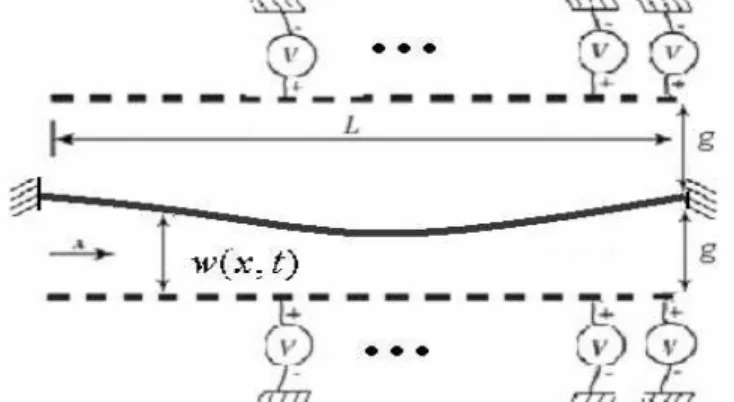
2. SYSTEM DESCRIPTION

The studied system consists of a continuous deformable microbeam, clamped on both extremities and subjected to distributed time-variant electrostatic forces generated by the application of distributed time-variant voltages on N

electrodes chosen from the two sets disposed on the both sides of the microbeam.

Fig. 1. The deformable microbeam surrounded with two sets of N electrodes on each side, subjected to different variant distributed voltages.

The two sets are necessary to make possible the generation of attractive forces on both directions depending on the calculated control signals. The 1st_{order approximative}

relation linking the electrostatic force to the applied voltage on a determinate position x, is:

2 2 0 )) , ( ( ) , ( . 2 1 ) , ( t x w g t x u S t x f e − = ε (1)

where Se is the electrode surface, u( tx, ) is the applied instantaneous voltage, g is the initial gap between the

microbeam and the electrode and w( tx, ) is the transverse

displacement of the microbeam which is measured using the capacitive principle. The 1st order approximative equation

relating the measured capacitance to the displacement is:

) , ( ) , ( 0 t x w g S t x C e − = ε (2)

When on a fixed instant t, an electrode is used as an

electrostatic actuator and is subjected to a voltage, the other one is connected to a capacitive electronic measurement circuit, while a low voltage is applied on the microbeam for the detection aim.

The electric measurement circuitries as well as the ADC converters add noise to the output signals. Smaller are the electrode surfaces, smaller are the measured capacitance magnitudes with the same electric noise and thus the signal to noise ratio decreases with the increasing number of the electrodes used. In addition, the complexity of fabrication, miniaturization and computation increases and the controller becomes more difficult to integrate when using classical control methods. In the other hand, the bigger is the number of the electrodes and the more continuous is the generated local forces along the microbeam which allows more precise reference tracking. In this work, 1000 electrodes are used.

3. DEFORMATION MODELLING

The behaviour of the deformation of a rectangular microbeam with length l, thickness e, width h, subjected to an external

distributed strength obeys to the following differential equation: 2 2 4 4 ₍ _, ₎ )) , ( ( ) , ( x t x w t x w T x t x w EI ∂ ∂ + ∂ ∂ ) , ( ) , ( ) , ( 2 2 t x f t t x w S t t x w b = ∂ ∂ + ∂ ∂ + ρ (3)

with S=h.e the transversal section of the beam, E the

Young’s modulus, I the moment of inertia, ρ the density, b

the friction coefficient associated to the interaction with the surrounding fluid, w( tx, ) the time dependent transverse

displacement at position x, and T(w) is the stress associated to

the elongation of the beam.

Fig. 2. The clamped-clamped microbeam with dimensions l, h and e.

Following Galerkin procedure of standard modal analysis,

) , ( tx

w _{can be written as:}

∑

₌ = n k ak t wk x t x w 1 (). ( ) ) , ( (4)

where wk(x) are the n mode shape vectors and ak(t) the

dynamic related coefficients. A solution of this equation, with respect to the boundary conditions and considering a

(4)

clamped-clamped microbeam, is shown in (Kharrat et al., 07)

and leads to the modal shapes space wk(x) shown in fig. 3.

Using equation (4) in (3) and projecting on each vector wi,

we get n equations representing the n modes that can be

written in a matrix form:

F X M X B X N KX + ( )+ &+ &&= (5) where [ ]T n t a t a t a X= 1() 2() L () ,M =ρ.S.In,               = 4 4 2 4 1 0 0 0 0 0 0 n EI K λ λ λ L O M M L ,             = n b b b B 0 0 0 0 0 0 2 1 L O M M L ,               = n w f w f w f F _M 2 1

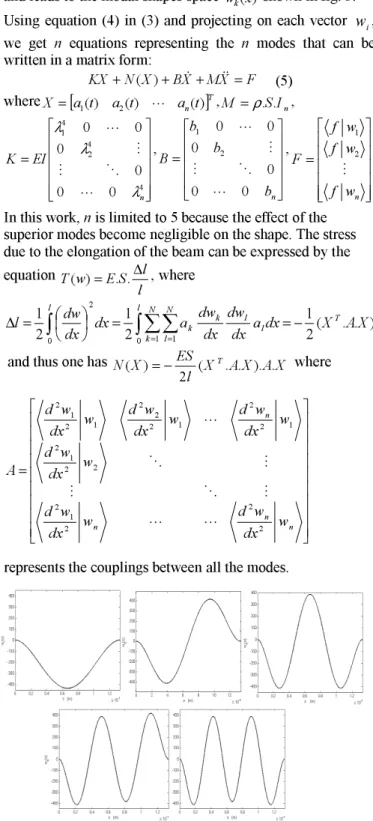
In this work, n is limited to 5 because the effect of the

superior modes become negligible on the shape. The stress due to the elongation of the beam can be expressed by the equation l l S E w T( )= . .∆ , where ) . . ( 2 1 2 1 2 1 0 1 1 2 0 X A X dx a dx dw dx dw a dx dx dw l T l l l N k N l k k l − = =       = ∆

_∫

_∫∑∑

= =

and thus one has X AX AX l ES X N ₍ T_. _. _). _. 2 ) ( =− where                       = n n n n w dx w d w dx w d w dx w d w dx w d w dx w d w dx w d A 2 2 2 1 2 2 21 2 1 2 2 1 22 2 1 21 2 L L M O M M O L

represents the couplings between all the modes.

Fig. 3. The first five wk(x) representing the first five modal

shapes of the microbeam.

4. "REGULATOR PROBLEM" AND "LTR" TECHNIQUE FOR MODE-BASED-CONTROL

To control the microbeam shape having the N actuators with

the displacements reference vector and the displacements measures in each position along the microbeam, a

rudimentary idea is to calculate each local tracking error and to use it as controller input for the computation of the required local force to be applied, at a cost of a huge network of N controllers. Also, one will be dealing with the equation

(1) directly which has unknown coupling terms with the other displacements and no desired exact dynamics can be imposed on displacements responses. By controlling the dynamic mode coefficients ak(t), the sum of the modulated shape

vectors

_∑

= = n k ak t wk x t x w 1 (). ( ) ) ,

( will lead to the desired shape

when all ak(t)→akr, the reference mode coefficients. Any vibrating shape reference is described by different sinusoidal dynamic coefficients whose model is added to the system state space model to obtain the so-called standard model. To take into consideration a possible disturbance action on the input, a model of a constant disturbance d is

also added so that the standard model becomes:

k kr kr k k k kr kr k k f m a ad a a m b m k m a ad a a                 +                                 − − − =                 0 0 0 / 1 0 0 0 0 0 1 0 0 0 0 0 0 0 0 0 0 0 0 / / 0 0 / 1 1 0 2 _& & && & & && & ω

ω is the vibration pulsation. This standard model with its

tracking errors e and outputs y can be written as:

u B x x A A A x x       +             =       0 0 1 2 1 22 12 11 2 1 & & _[ _] k kr e e _x a a x C C e _= −      = 2 1 2 1 ,

[

]

_      =       = kr k y y _a a x x C C y 2 1 2 1

where x1 are the system states and x2 are the exosytstem states (disturbance and reference).

                    22 12 11 0 , A A A C C y e is observable, ( ) 1 11, B A is stabilizable and 22

A is unstable. Finding a regulator K that tends e towards 0

for any initial conditions and keeps the closed loop system stable is what was referred to as “regulator problem with internal stability” (RPIS) by (Wonham 1985). If the solutions

(

_∈_ℜ2×3_, _∈_ℜ1×3

)

a

a T

F of the following equations:    = + − − = + + − 0 2 1 1 12 22 11 e a e a a a C T C F B A A T T A ₍₆₎

exist, than the regulator of an FSF (Full State Feedback) – observer type with the gains F =[F1 F1Ta +Fa] where F1 is such that A11+B1F1 is stable and K is such that A−KC is stable, guaranties the stability of the closed-loop system and the reference tracking. Resolving these equations in our case gives _      − − = 1 0 0 0 1 0 a T and Fa=

[

−1 kk−mω2 bk

]

.

(5)

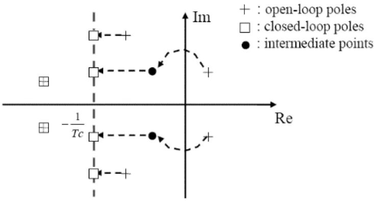
Having the appropriate standard model (the number of reference and disturbance states included in the standard model is equal or bigger than the number of measured output) a robust asymptotic reference tracking can be achieved (De Larminat, 1995). For robust stability, one has to adjust the gains F1 and K=[Kxd Kr] for system + disturbance (Ksd) and reference (Kr) states observation. The LTR technique was used to choose these gains:

Considering possible access to the all the states, and by choosing the closed-loop poles that ∀i and ∀w,

i i jw po

pc

jw− ≥ − , where pci and poi are respectively the closed-loop and open-loop poles, one has

1 1 1 _≤ − −

∏

= = n i i n i i pc jw po

jw _{thus the loop sensibilty}

1 ) (jw ≤ S , 1 ) ( 1+ ≥

⇒ L jw , ∀w which means that the loop transfer

function L( jw) is always outside the circle of centre -1 and

beam equal to 1 in the Nyquist diagram, which guaranties good stability margins. This can be done by choosing a parameter −1/Tc which defines the axis in the left side of the complex space (De larminat, 2000). After projection of the unstable open-loop poles to the left quadrant, the projections on the −1/Tc axis of those who are on its right + those who are on its left represent the closed-loop system poles. In other words, Tc represents the desired response speed for the closed-loop system. Once the poles are chosen, resolving the Ackerman’s formula allows to obtain the gains of F1.

Fig. 4. The poles placement technique that assures the robust stability of the closed loop system.

When we don’t have access to all the “system+disturbance” states (which is our case), an observer is needed which leads to a new Ln( jw). For an exact LTR, this latter is equal to the

target one but this can only be obtained with a derivative regulator that amplifies the noise influence on control signals and outputs. That’s why an asymptotic LTR is adopted and a parameter −1/To is chosen, which defines the axis in the left side of the complex space. After projection of the unstable open-loop zeros to the left quadrant, the projections on the

o

T / 1

− axis of those who are on its left + those who are on its

right + the remaining observer poles set on −1/To, represent

the observer poles. It was proven that when To →0, and the

observer poles are set exactly on the open-loop zeros and the remaining ones on −∞ and so Ln(jw)→L(jw) (Saberi et al.,

1993). Generally, To is chosen 3, 5 or 10 times smaller than c

T. Once the poles are chosen, resolving the Ackerman’s

formula allows to obtain the gains of Ksd. As for the reference observer’s poles, they can be chosen with dynamics faster than those defined by the reference vibration frequency, which allows precise reconstruction of the reference and of its derivative. Using Ackerman’s formula, the gain of Kr is calculated.

The two parameters Tc and To are chosen by taking into consideration the control specifications and the reference dynamics. The smaller Tc is and the faster is the response speed which can be useful in case of disturbance rejection. In addition, robustness via the parameters uncertainties is improved. But, in the other hand, the noise influence is higher on output and on control signal and big solicitation of the actuators is predicted. Once the target loop is selected with

c

T, To is tuned so that we approach the specified performances and the robustness of the target loop but without having an important derivative action, to obtain a better noise rejection. Guarantying one of the two objectives is easy to obtain, but having both on the same time is much more complex and a compromise must be done.

This control scheme is applied to each of the five dynamic coefficients of the first five modes, requiring five regulators instead of N ones. The calculated control signals fk allow the calculation of the distributed desired electrostatic force

∑

₌ = n k fk t wk x t x f 1 (). ( ) ) ,

( and the required local voltages to be

applied on the N electrodes are calculated by

S t x f t x w g t x u 0 ) , ( 2 . ) , ( ) ,

( = − _ε and are applied on the higher

electrode if f(x,t)>0, and on the lower one if f(x,t)<0. A

problem is that w( tx, ) are the noisy measurements so the

calculated voltages u( tx, ) will not generate exactly the

required forces for the real displacements. This limits the intended advantages just when these required forces have big magnitudes which amplify the noise in the calculated voltages.

5. PRACTICAL CASE OF SIMULATIONS AND TESTS The microbeam model is implemented in Simulink/Matlab with a length l=13,35µm, a width h=0.2µm and a thickness

m

e=0.2µ . The moment of inertia is then _I₌_h._e3/12. The

gap between the electrodes is g=0.5µm, So the parameters

of the model are: _. _. 4 k k EI k = λ , Qm k b k k . = and m=ρ.e.h

with _E₌₁₆₉_.₁₀9, _ρ₌₂_.₂₃₂_.₁₀3 and Q₌₄₀₀₀ for all the modes. λ are the calculated eignevalues of the modes and

(6)

one has (λkl)=[4.73 7.85 10.99 14.13 17.27 L]

.

The

resonance frequencies of the 5 modes go from 10 Mhz to 134 Mhz. The chosen reference coefficients define a certain shape, vibrating with a frequency f = 10 Mhz. The couplings

between the displacements represented by the couplings between the different modes are taken into consideration. The electrical noise is modelled as a white noise of spectral power equal to 10−5aF / Hz for a sampling frequency of 1 GHz. A

constant disturbance is added to the electrostatic forces. In addition to all these specifications, a modification of 20% on all the microbeam's parameters were considered to test the robustness of the control scheme even in case of noisy measurement and disturbing environment with uncertain systems.

Depending on their initial dynamics and parameters, different c

T and To are chosen for the different modes and are shown in table 1.

Table 1. Control and observation parameters

Mode num

Tc

To

1

st

_mode

_2.10

-8

_Tc/4

2

nd

_mode

_1.10

-8

_Tc/5

3

rd

_mode

_8.10

-9

_Tc/4

4

th

_mode

_7.10

-9

_Tc/4

5

th

_mode

_5.10

-9

_Tc/3

The results obtained for the shape tracking without disturbance application are shown in the following figures:

Fig. 5. The 5 dynamic coefficients ak of the noisy measured

shape used as regulators inputs (on top) compared to the real shape coefficients of the closed-loop system (on bottom). When a constant disturbance is added to the actuators forces as an instantaneous step (which can represent a mechanical shock or a curt acceleration), the designed controllers exhibit good performance (for the same values of Tc, To) and results are shown in fig. 9.

Fig. 6. The comparison between the reference shape (blue curve) and the output shape (red curve) of the microbeam on a fixed instant tf (on top) and the correspondent desired force

distribution of the actuators (on bottom).

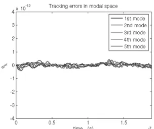
Fig. 7. The modal tracking errors coefficients for the 5 modes. One can notice that errors don't exceed the 10% of the reference coefficients.

6. CONCLUSION

This paper details the design of a fully integrable control loop for a microbeam dynamic shaping by electrostatic actuation done with two sets of 1000small electrodes disposed on both sides of the microbeam. First of all, the detailed modelling of the structure using modal analysis is presented. Then the control problem of each of the first five modes was formulated as a “regulator problem with internal stability” for extended systems models containing the modes dynamics models as well as the “exosystems”, considering a known reference trajectory after projection on the modal space of dimension 5, and a constant disturbance to be rejected. Then the controllers are designed by placing the poles of the closed-loop systems such that good robustness, stability and performance are expected and observers are designed accordingly to the “LTR” technique to approach the closed target loops. This procedure was successfully simulated on Matlab and control specifications are obtained.

(7)

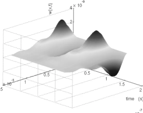
Fig. 8. Microbeam shape evolution with time.

Fig. 9. The 5 dynamic error coefficients ek in case of

disturbance application on force inputs, having the same Tc

and To chosen for other control specifications.

REFERENCES

Chu L.L., Que L., Li M.H. and Gianchandani Y.B. (2002), “Measurements of material properties using differential capacitive strain sensors”,

J. MEMS

, Vol. 11 (5), pp.

489-498.

De Larminat, P. (1995), "The sufficient duplication principle : an alternative issue to the internal model principle",

IFAC Conference On System Structure and

Control

, Nantes, France.

De Larminat Ph (2000),

“Contrôle d’état standard”

, Collection pédagogie d’automatique, Hermès, Paris. Huonker M, Waibel G, Giesen A and Hugel H (1997), “Fast

and compact adaptive mirror”,

Proc. SPIE-Int. Soc.

Opt. Eng

.

3097, pp. 310-319.

Isobe D and Nakagawa H (1998), “A Parallel Control System for Continuous Architecture Using Finite Element Method”,

Journal of Intelligent Material

Systems and Structures

, Vol. 9, No. 12, pp.

1038-1045.

Irschik H (2002), “A review on static and dynamic shape control of structures by piezoelectric actuation

”,

J Eng

Struct

, Vol. 24, pp.5–11.

Kharrat C, Colinet E and Voda A (2007), “Microbeam dynamic shaping by closed-loop electrostatic actuation using modal control”,

3rd IEEE Conference on

Ph.D. Research in Microelectronics and

Electronics, PRIME

-

2007.

Krommer M. and Irschik H. (2007), “Sensor and actuator design for displacement control of continuous systems”,

Smart Structures and Systems

, Vol. 3, No. 2, pp.

147-172.

Liu C H, Hagood N W and Hall E K (1993), “Adaptive lightweight mirrors for the correction of self-weight and thermal deformations”

ASME

,

Aerosp. Div.,

Adapt. Struct. Mater. Syst

. 35, pp. 171-183.

Luo Q and Tong L (2006), “High precision shape control of plates using orthotropic piezoelectric actuators”,

Finite

Element. Anal. Des

.

42, 1009-20.

Luo O. and Tong L. (2007), “A segment based sequential least squares algorithm with optimum energy control for tracking the dynamic shapes of smart structures”.

Smart Mater. Struct

.

Vol. 16, pp. 517–1526.

Min Liu, Kurt Maute and Dan M. Frangopol (2007), “Multi-objective design optimization of electrostatically actuated microbeam resonators with and without parameter uncertainty”,