Airline-Driven Performance-Based Air Traffic Management:
Game Theoretic Models and Multicriteria Evaluation
The MIT Faculty has made this article openly available.
Please share
how this access benefits you. Your story matters.
Citation
Evans, Antony et al. “Airline-Driven Performance-Based Air Traffic
Management: Game Theoretic Models and Multicriteria Evaluation.”
Transportation Science 50,1 (February 2016): 180–203 © 2016
INFORMS
As Published
http://dx.doi.org/10.1287/trsc.2014.0543
Publisher
Institute for Operations Research and the Management Sciences
(INFORMS)
Version
Author's final manuscript
Citable link
http://hdl.handle.net/1721.1/112157
Terms of Use
Creative Commons Attribution-Noncommercial-Share Alike
1
Airline-Driven Performance-Based Air Traffic Management: Game Theoretic
Models and Multi-Criteria Evaluation
Antony Evansa, Vikrant Vazeb and Cynthia Barnhartc aUCL Energy Institute, University College London bThayer School of Engineering, Dartmouth College
cDepartment of Civil and Environmental Engineering, Massachusetts Institute of Technology
Abstract
Defining Air Traffic Management as the tools, procedures and systems employed to ensure safe and efficient operation of air transportation systems, an important objective of future air traffic management systems is to support airline business objectives, subject to ensuring safety and security. Under the current model for designing air traffic management initiatives, the central authority overseeing and regulating air traffic management in a region makes trade-offs between specified performance criteria. The research presented in this paper aims instead to allow the airline community to set performance goals and thus make trade-offs between different performance criteria directly, before specific air traffic management strategies are determined. We propose several approaches for collecting inputs from airlines in a systematic way and for combining these airline inputs into implementable air traffic management initiatives. These include variants of averaging, voting and ranking mechanisms. We also propose multiple criteria for evaluating the effectiveness of each approach, including Pareto optimality, airline profitability, system optimality, equity, and truthfulness of airline inputs. We apply a game-theoretic approach to examine the potential for strategic (gaming) behavior by airlines. We offer a broad evaluation of each approach, first by providing some theoretical insights, and then by simulating each of the approaches for a generic system using Monte-Carlo methods, sampling values for input parameters from a wide range. We also provide an indication of how the approaches might perform in a real system by simulating ground delay programs at two airports in the New York City area. We first apply a simplified model that simulates the process of selecting only planned end times of a ground delay program, using Monte-Carlo methods. Next, we apply a more detailed model that simulates the process of selecting planned end times and reduced airport arrival rates. Finally, we characterize the effectiveness of each of the considered approaches on the proposed criteria and identify the most desirable approaches. We conclude that voting schemes, which score highly on all criteria (including airline profitability, system optimality and equity), represent the most promising approaches (among those considered) to elicit airline preferences, thereby allowing the central authority to design air traffic management initiatives that optimize system performance while respecting the objectives of airlines.
Keywords
2
1. Introduction
Air Navigation Service Providers (ANSPs), such as the Federal Aviation Administration (FAA) in the United States and EUROCONTROL in Europe, are the central authorities responsible for safe and efficient operation of our air transportation systems. In order to ensure these goals, ANSPs employ various tools, procedures and systems, which together are termed Air Traffic Management (ATM). ATM systems in the U.S. and Europe are currently poised for a major overhaul, under projects titled Next Generation Air Transportation System (NextGen) in the U.S., and Single European Sky ATM Research (SESAR) in Europe. An important objective of future ATM systems as envisioned by the FAA is supporting the business objectives of airlines, subject to ensuring safety and security (JPDO, 2007; FAA, 2011). In addition to safety and security, airlines value many different operational aspects of the air transportation system, such as capacity, efficiency, flexibility, predictability etc. Better availability of sufficient capacity in the various components of the system reduces or eliminates congestion related delays. Greater efficiency in resource utilization translates into reduced operating costs. Greater flexibility in scheduling operations enables airlines to make appropriate changes closer to departure times, as their needs evolve with time. Better predictability, which refers to the reliability of the system to deliver on planned performance, leads to more certainty about future operations, which in turn helps airlines plan better. Different airlines might value these different performance criteria differently.
An ANSP may support airlines’ business objectives by designing Traffic Management Initiatives (TMIs) in such a way as to maximize a single performance goal or some pre-defined combined measure based on multiple performance criteria, subject to ensuring safety and security. Here, performance goal refers to the quantified value, based on some defined metric, of a performance criterion. However, an ANSP cannot typically maximize all performance goals simultaneously, and must identify an appropriate trade-off between them. For example, consider a Ground Delay Program (GDP), a common TMI implemented by the FAA to control the flow of aircraft into an airport by delaying flights destined for that airport at their respective origin airports. A GDP is typically implemented for a period of time when increased aircraft spacing is considered necessary between landing aircraft, to ensure safety, and is often associated with adverse weather. However, weather forecasts are uncertain, so the point when conditions improve and additional spacing is no longer necessary is usually difficult to predict. Setting a GDP end time to be optimistically early maximizes the airport capacity and therefore throughput, because inbound flights are not delayed at their departure gates any longer than necessary. Therefore, no matter when conditions improve, and the airport capacity can be returned to the normal level, there are aircraft positioned to land. However, last minute extensions may have to be made to the GDP if the adverse weather continues longer than was forecast, potentially requiring airborne holding. So an early GDP end time would be at the expense of predictability (in addition to safety concerns and fuel costs associated with airborne holding). To maximize predictability, the GDP end time should be set conservatively late, allowing airlines to be confident that the GDP would not be extended. But this would be at the expense of throughput, as capacity might be underutilized if conditions were to improve earlier than the set GDP end time. There is therefore a trade-off between throughput and predictability. Different airlines might have different preferences for prioritizing throughput over predictability. For example, for an airline operating a frequent shuttle service with low load factors, which allows easy
3
rebooking of passengers and easy reassignment of aircraft, some throughput reduction is not as detrimental as operating an unpredictable schedule. On the other hand, for an airline with lower frequency and higher load factors, for which delay recovery is difficult, high throughput may be preferred to predictability so that the airline does not have to cancel flights. The primary motivation for our research is to investigate various approaches for ANSPs to determine the trade-off between performance criteria, based on inputs (i.e., preferences) from airlines. We apply our research specifically to the case of GDPs.
In the existing literature, supporting airline preferences has typically been studied at the level of individual flight trajectories, through trajectory-based initiatives. In such initiatives, airlines are, for example, given authority to modify their own flight trajectories in a far- and mid-term time horizon to avoid an identified constraint, such as a region of airspace with high traffic or a region impacted by weather (e.g., Garcia-Chico
et al., 2008). Alternatively, airlines are given the opportunity to provide the ANSP with multiple prioritized
flight trajectories, individual flight priorities, or route priorities (e.g., Sheth and Gutierrez-Nolasco, 2008). In this paper, we consider accommodating airline preferences at the more aggregate level, shifting the focus from flight trajectories to overall system performance. To the best of the authors’ knowledge, ours is the first study that addresses the challenge of supporting airline preferences at a system level. Such a performance-based ATM system would be capable of making trade-offs between different performance criteria, such as capacity, efficiency, flexibility, predictability etc., at the system level, and could account for the system-level performance preferences of different airlines. The chosen system performance objectives would then serve as the basis for deciding on specific parameters, such as the length, scope and magnitude of TMIs, that include GDPs, Ground Stops, Miles-in-Trail (MIT) restrictions, traffic re-routes, etc.
The performance of the U.S. National Airspace System (NAS) is typically measured by the number of delayed flights and by the length, scope and magnitude of TMIs. The length of a GDP, Ground Stop, MIT restriction or re-route typically refers to the planned duration of the initiative. In the case of a GDP, Ground Stop, MIT restriction or re-route, scope refers to the subset of flights impacted by the initiative. For example, in the cases of a GDP or Ground Stop, scope refers to the set of flights delayed on departure as a consequence of the initiative. This set is comprised of all flights whose destination is the constrained airport and whose origins are within a specified maximum distance from the constrained airport. The magnitude of a GDP refers to the specified airport arrival rate (AAR) at the destination airport, which in the case of a Ground Stop is zero. The magnitude of a MIT restriction is the actual in-trail spacing required of the traffic, while the magnitude of a re-route can be considered to be how far from the planned flight trajectory the reroute takes the traffic. These values, however, do not represent the performance of the system per se, but are rather indicators of aspects of the system performance (FAA, 2011). They are also inadequate to describe differences in system-level preferences and requirements of different airlines. It is therefore important to identify what the performance criteria of airlines are, and to describe them in quantifiable terms. The International Civil Aviation Organization (ICAO, 2005) lists performance criteria, or the “expectations of the ATM community”, as follows: access and equity, capacity, cost-effectiveness, efficiency, environment, flexibility, global interoperability, participation by the ATM Community, predictability, safety, and security. In this paper, we focus directly on a subset of these performance criteria rather than dealing with indicators of aspects of performance, as has been done traditionally. The reader is referred to Liu and Hansen (2012) for an example of how performance goal vectors can be expressed as a function of these indicators of aspects
4
of performance. A performance goal vector refers to a vector with individual components that are the values or goals for specific performance criteria, such as capacity, predictability etc. In this paper, we make use of the expressions of capacity and predictability developed by Liu and Hansen (2012) when analyzing specific TMIs in Section 5.
Given the differences in the valuation of these performance criteria by different airlines, an approach or a mechanism is needed to reconcile their competing preferences. In contrast, in the existing ATM system, the
ANSP has sole responsibility for determining these offs when designing TMIs. For example, the
trade-off of throughput and predictability is determined in designing a GDP with the ANSP selecting the GDP end time, as described above, as well as scope and magnitude. The research presented in this paper aims instead to allow the airline community to influence TMI design by providing preferences in advance of the TMI design and implementation. In so doing, the ANSP can then design TMIs that capture airline preferences in the most effective way. A primary aim of this research is to design and assess various candidate mechanisms for this process, and demonstrate their applicability through general experiments and specific, real-world motivated case studies.
Consistent with the FAA objective of supporting airlines’ business objectives, a large amount of research has been focused on formulating and solving the problem of system optimality in air transportation (e.g., Odoni and Bianco, 1987; Bertsimas and Stock-Patterson, 1998, 2000; Lulli and Odoni, 2007). In effect, these studies describe ways in which airlines and the ANSP might attempt to maximize total airline profits and minimize system cost by trading off performance goals, without compromising safety and security. The ICAO performance criteria that are most likely to be traded in such a scenario are capacity, efficiency, predictability and flexibility. Because each airline may prefer a different trade-off, it becomes important to ensure equity in how each airline’s preferences are combined to set the final system-wide performance goals. It is noted that, as described by Bertsimas et al. (2011), the trade-off that minimizes system cost might not, in fact, be equitable, depending on how equity is defined. This is further complicated by the fact that when an airline requests certain performance goals, the request might not, in fact, represent the airline’s true preferences. In other words, an airline might not be truthful about its preferences, and might behave strategically, in effect gaming the system, requesting performance goals different from its true preference in order to draw the finally selected system performance goals closer to its desired outcome. This can have significant consequences for equity, because, while it might appear that a solution is equitable based on the submitted preferences, it could be far from it. Furthermore, if airlines game severely (requesting solutions far from their true preferences), the ANSP is provided with an inaccurate picture of the airlines’ preferences, and therefore of how well it is serving the airlines. Therefore, in this paper, in addition to airline profitability and system optimality, we also use equity and truthfulness to assess the effectiveness of any mechanism under consideration.
As mentioned earlier, due to safety and security concerns, not all of the relevant system-wide performance criteria, such as capacity, efficiency, predictability and flexibility, can be simultaneously maximized. This is especially true in cases of high traffic and/or adverse weather. Thus, there is a tradeoff between these different system-wide performance goals. An increase in one performance goal beyond a certain level necessarily requires a reduction in another. We define the trade space as the set of all combinations of
5
system-wide performance goals that are feasible, subject to ensuring safety and security. Note that the trade space as well as the performance goals are defined at the system level and all else being equal, each airline is assumed to prefer a higher value of a system performance criterion at least as much as a lower value of the same performance criterion. A subset of the boundary of the trade space is Pareto efficient, in that, for any point A in this Pareto efficient subset of boundary points, there does not exist another point B in the trade space such that the value of each performance criterion at point B is at least as high as the value of that performance criterion at point A and the value of at least one performance criterion at point B is strictly greater than the value of that performance criterion at point A. We define this subset of the boundary of the trade space as the Pareto frontier.
2. Contributions
In this paper, a number of contributions are made to performance-based ATM research:
This is the first study that investigates various approaches to allow the airline community to set the system-level performance goals of the ATM system, and thus make trade-offs between performance criteria directly. We do this using a rigorous game-theoretic approach, which identifies the potential for gaming by airlines.
We propose several approaches for collecting inputs from airlines in a systematic way and for combining these airline inputs into implementable TMIs. These include an approach which takes a weighted average of the airline-preferred performance goals; an approach that pushes the weighted average of the airline-preferred performance goals out to the Pareto frontier; an approach that makes a weighted random choice of airline-preferred performance goals; an approach that allows airlines to rank preferred performance goals; and an approach in which airlines vote on preferred performance goals.
We propose multiple criteria for evaluating the effectiveness of each approach to performance-based ATM, including Pareto optimality, airline profitability, system optimality, equity, and truthfulness of airline preferences.
By first performing a theoretical analysis and then simulating each of the approaches for a generic system using Monte-Carlo methods (sampling values for input parameters from a wide range), we offer a broad evaluation of each approach to performance-based ATM.
We also apply the approaches to more realistic cases in which we simulate GDPs at Newark Liberty International airport (EWR) and at LaGuardia airport (LGA), both in the New York City area. Two models are run: one simplified GDP model that simulates decisions regarding the planned GDP end time, and is applied using Monte-Carlo methods; and a second more detailed model that simulates decisions regarding both planned GDP end time and GDP magnitude, and is run for a single GDP case at each of EWR and LGA, respectively. The results of these simulations provide an indication of how the approaches would perform in a real system, and how the results differ from those for the generic experiments.
6
Finally, we characterize the effectiveness of each of the considered approaches on the proposed criteria and identify the most desirable approach accordingly. Taking a weighted average of the user preferred performance goal vectors, making a weighted random choice of the user preferred performance goal vectors, and voting on ANSP provided candidate performance goal vectors were all found to be reasonable candidates for practical implementation. However, the voting scheme shows particular promise, scoring highly on all criteria.
3. Framework
Figure 1 provides a high level view of the process to be investigated.
Figure 1. Architecture for process by which performance goals are set
The ultimate output of the process is a set of system-wide performance goals (upper right-hand box in Figure 1) that would be used by the ANSP to set specific TMIs. A possible form of these performance goals is described in Section 5. This set of performance goals could be for a single TMI within a single resource, such as the GDP at an airport described in the example in Section 1. Alternatively, the set of performance goals could be for multiple initiatives with multiple resources, or for the national airspace system as a whole. The process may start with an initial set of candidate performance goals suggested by the ANSP, or directly with inputs from each airline (set of boxes on upper left in Figure 1), which would be the performance goals preferred by each airline. A performance goal resolution process would then take the inputs from all airlines, confirm the feasibility of each input, and identify a set of system-wide performance goals by combining these different inputs in some way. The ANSP can then provide individual airline feedback, which would be a description of how the system-wide performance goals translate into changes in each specific airline’s operational plan, e.g. delays to individual flights scheduled to arrive at an airport under a GDP. This allows each airline to assess the impact of the system-wide performance goals on its operational performance, such as propagated delays, passenger and crew schedule disruptions, additional fuel burn, etc., through an airline
assessment process. In this process, each airline considers the feedback and determines what adjustments to
make to its input in order to influence the system-wide performance goals in such a way as to improve its own operational performance. This feedback loop can be executed several times until an equilibrium is reached, where no airline can unilaterally adjust its own inputs to produce a “better” set of system-wide
Performance Goal Resolution Airline 1 Feedback Airline 1 Assessment Airline 1 Input System-Wide Performance Goals
7
performance goals (better being in terms of the performance objectives of that airline). This represents a pure strategy Nash equilibrium, a concept commonly used in game-theoretic literature to model situations with multiple, interacting, autonomous decision makers. We will use this concept to model the outcome of this iterative process.
The airline inputs and the performance goal resolution process may take a number of different forms. In this paper, different forms are studied in order to identify which has the best characteristics for setting system-wide performance goals. Each is described in detail in Sections 3.1 and 3.2 respectively. This is followed by a description of the metrics used to evaluate all approaches in Section 3.3.
3.1 Form of Airline Inputs
In this paper we analyze two forms of airline inputs:
1. A preferred performance goal vector – Each airline k simply specifies its preferred performance goal vector (Ik). This airline input is most applicable to a continuous trade space. In the example of a GDP
described in Section 5.2, this input would take the form of each airline’s preferred trade-off between capacity and predictability, using some pre-defined metrics. This trade-off could be input in the form of the parameters of the GDP (such as GDP end time and AAR), or it could be input in the form of capacity and predictability metrics that are calculated from these parameters. For example, a metric describing capacity could be the ratio of expected throughput, given known uncertainty in the GDP end time, to the maximum throughput that would be possible with perfect information. Similarly a metric for predictability could be the ratio of the expected flight delay assuming the GDP were to end as planned, to the expected delay given known uncertainty in the GDP end time. These metrics are described in more detail in Section 3.3.
2. Votes or rankings on a set of candidate performance goal vectors – Each airline k specifies its preferences in the form of votes or rankings Ikp for each of the P candidate performance goal vectors
𝐺𝑝: 𝑝 ∈ {1, 2, … , 𝑃}. This airline input is most applicable for a discrete trade space, in which only a
finite set of candidate performance goal vectors are valid or are under consideration. In the GDP example described in Section 5.2, this input would take the form of either a vote or a ranking, from each airline, for each of the candidate vectors.
3.2 Performance Goal Resolution Approaches
The ANSP determines the system-wide performance goal vector (G*) by combining all airline inputs according to a defined resolution approach. Five different approaches are analyzed in this paper. For each approach described below and each airline k, the weights (wk) are proportional to some non-decreasing
function of the number of operations of k impacted by the initiative.
1. Taking a weighted average of all airline-preferred performance goal vectors – This is a simple and intuitive way of combining continuous-valued airline inputs. After each airline k has specified its preferred performance goal vector Ik, a weighted average performance goal vector is calculated.
8
G* = k wk Ik (1)
In the case of the GDP example, if specific parameters of the GDP representing capacity and predictability are traded off, such as GDP end time T and AAR C (specifying the duration and magnitude of the GDP), this equation is represented by (2), with the inputs from each airline k represented by Tk and Ck, and the system-wide solution represented by T* and C*.
[T*, C*] = [k wk Tk, k wk Ck] (2)
The iterative framework described above is applied, allowing airlines to modify their preferred performance goal inputs according to inputs from other airlines. The process is continued for a set number of iterations, or until convergence to an equilibrium, as described in Section 5.
A sample outcome of such an iterative process is illustrated in Figure 2 for the case of two airlines and two performance criteria. In this example, the Pareto frontier is represented by an arc of a circle centered at the origin, and concave increasing quadratic payoff functions are assumed for each airline. Truthful solutions for both airlines are shown (as red and blue circles). A line of constant payoff for a particular airline and payoff value is defined as the set of all performance goal vectors corresponding to that payoff value for that airline. In Figure 2 it represents the range of trade-offs between the simulated performance goals that would result in identical payoff to the airline. As we move towards the upper right of the figure, increasing the values of both performance goals, airline payoff increases. Therefore, the truthful solutions at which each airline maximizes its payoff lie where the lines of constant payoff are tangent to the Pareto frontier, as shown. Airline inputs at equilibrium are shown respectively by red and blue ×s for the two airlines. These are the results of the aforementioned iterative process where each airline maximizes its payoff, given the input of the other airline. In the case of this sample instance, these points differ from the truthful solutions, because each airline is able to increase its payoff from the system-wide performance goal vector by gaming. As can be seen, each airline attempts to “pull” the system-wide solution towards its truthful solution. The final system-wide performance goal vector, calculated as a weighted average of goal vectors input by each airline, is also shown on the figure (black ×). This is an interior point, and therefore not Pareto optimal.
9
Figure 2. Sample result applying weighted average of all user preferred performance goal vectors.
2. Taking a weighted average of all airline-preferred performance goal vectors (as in 1), and pushing the
result out to the Pareto frontier – This approach is similar to that presented above but avoids the issue
of the combined output vector being in the interior of the trade space, and therefore not Pareto-optimal. In the case of a convex trade space where this Pareto frontier is non-linear, a weighted average of airline-preferred inputs might not fall on the Pareto frontier itself. After each airline k has specified its preferred performance goal vector Ik, a weighted average performance goal vector is
calculated in the same way as in approach 1, above. This is then shifted out to the Pareto frontier. This shift can be done in many different ways. One reasonable approach is to do this in such a way as to maintain the same ratios of the values of each performance goal, generating a new system-wide performance goal vector that is on the Pareto frontier. This approach is also most applicable for a continuous trade space, for which the airline inputs are preferred performance goal vectors. Mathematically, this can be represented as:
G* ParetoFrontier (3)
such that: Gm* / Gn* = Gm’ / Gn’ for all m, n
where G‘ = k wk Ik
Note that this point, G*, on the Pareto frontier will always be unique because if there are two such points with the same ratio of the values of each performance goal then one of the two points will have a lower value of each performance goal compared to that for the other point and hence the former will not lie on a Pareto frontier.
In the case of the GDP example described above, this equation would be represented as follows:
T* = f(C*) (4)
such that: T* / C* = T’ / C’
10
As in approach 1, the iterative framework described above is applied, allowing airlines to modify their preferred performance goal inputs according to inputs from other airlines. The process is continued for a set number of iterations, or until convergence to an equilibrium, as described in Section 5.
A sample outcome of such an iterative process is illustrated in Figure 3 for the case of two airlines and two performance criteria. Comparing Figure 3 to Figure 2, it is immediately clear that, by pushing the system-wide solution to the Pareto frontier, there is more gaming from both airlines. Airline inputs at equilibrium are shown respectively by red and blue ×s for the two airlines. These are the results of the aforementioned iterative process where each airline maximizes its payoff, given the input of the other airline. In Figure 3a, a case is shown in which the airline inputs (red and blue ×s) for both airlines fall at corner points. In Figure 3b, a case is shown in which only one of the airlines input is at a corner point. The other airline does not request a corner point because it is able to “pull” the system-wide solution to coincide with its truthful solution without moving to the corner point.
(a) (b)
Figure 3. Sample result applying weighted average of all user preferred performance goal vectors, pushed to Pareto frontier: (a) both airlines request corner point solutions, (b) only one airline requests
a corner point solution.
3. Making a weighted random selection of the airline-preferred performance goal vectors – The main motivation for considering this approach is that it eliminates strategic gaming behavior by the airlines, as we will see later in Section 6 and in Appendix B. After each airline k has specified its preferred performance goal vector Ik, one of the airline-preferred performance goal vectors Ik is randomly
selected for G*. The probability of each airline-preferred performance goal vector being selected is proportional to its weight wk. This approach is applicable for both continuous and discrete trade
spaces, for which the airline inputs are preferred performance goal vectors. Mathematically, this can be represented as:
11 where Pr( j = k ) = wk for all k
In the case of the GDP example, this equation would be represented as follows:
[T*, C*] = [Tj, Cj] (6)
where Pr( j = k ) = wk for all k
A sample result is illustrated for the case of two airlines and two performance criteria in Figure 4. As shown, the airline inputs and truthful solutions coincide. The reason for this is that airlines are not incentivized in any way to submit a different, non-truthful input because, if their solution is not chosen, their input does not affect the chosen solution in any way. Thus, they are incentivized to submit truthful solutions irrespective of how the probabilities are defined to randomly choose one of the airline inputs. This also means that the iterative framework described above is not necessary, as there is no incentive for any airline to change its preferred performance goal inputs based on other airline inputs. The system-wide goal vector (G*) is also always Pareto optimal because each user input is Pareto optimal.
Figure 4. Sample result applying weighted random selection of the user preferred performance goal vectors.
One disadvantage of this approach is that it does not account for the fact that the payoff of any chosen solution may vary significantly across airlines. The chosen solution may therefore have highly disproportionate impacts on each airline. A solution may exist that has the lowest overall impact on all airlines, but is not the most preferred solution for any of the airlines.
4. Ranking the candidate performance goal vectors based on airline preferences – After each airline k has specified its preferences for each of the P performance goal vectors Gp in the form of descending
ranks Ikp from P to 1 (P being the rank of that airline’s most preferred performance goal vector, and 1
the rank of its least preferred performance goal vector), the combined rank for each vector is calculated as a weighted sum of individual ranks assigned by different airlines to that vector. The
12
performance goal vector with the greatest combined rank is assigned to be the system-wide performance goal vector G*. This approach is most applicable for a discrete trade space, in which only a candidate set of performance goal vectors is valid. Mathematically, this can be represented as:
G* = Gq (7)
where q is such that Rq = max ( R1 , R2 , …,RP )
and Rp = k wk Ikp for all p{1, 2, …, P}
In the case of the GDP example described above, this equation would be represented as follows:
[T*, C*] = [Tq, Cq] (8)
where q is such that Rq = max ( R1 , R2 , …,RP )
and Rp = k wk Ikp for all p{1, 2, …, P}
As in approaches 1 and 2, the iterative framework described above is applied, allowing airlines to modify their rankings according to rankings from other airlines. The process is continued for a set number of iterations, or until convergence to an equilibrium, as described in Section 5.
Ranking is intuitive to understand and use, and unlike the first three approaches discussed above allows the airline to input its relative preferences for all the candidate performance goal vectors, instead of just specifying its single most preferred performance goal vector. Furthermore, an airline does not require exact knowledge of the payoffs of each performance goal vector to submit an input to the ranking mechanism. Instead airlines are only required to have a good idea of their comparative preference of one vector over the others. However, ranking is not devoid of drawbacks; the most significant is that the approach frequently does not converge, nor is a solution necessarily unique. Convergence is not guaranteed because airline rankings can alternate between two different rankings from iteration to iteration. In the cases run in this paper, this is a significant problem, with as little as 8% of runs converging (in the simplified GDP case at LGA). Convergence is highly dependent on the input parameters, and therefore different cases perform very differently (in contrast to the LGA case, 73% of runs converged in the simplified GDP case at EWR). In contrast, while convergence is not guaranteed for any of the other approaches (with the exception of taking a weighted random choice of user preferred performance goal vectors), convergence is significantly better under these other approaches than under ranking, as shown in Section 5.
5. Voting on the candidate performance goal vectors based on airline preferences – After each airline k has specified its preferences for each of the P performance goal vectors Gp in the form of Ikp votes, the
weighted sum of votes is calculated. This approach differs from ranking in that airlines can apply varying numbers of votes to each performance goal vector, according to their preferences, instead of just rank order. The total number of votes that can be assigned by an airline across different performance goal vectors is the same for each airline. The performance goal vector with the highest weighted sum of votes is assigned to be the system-wide performance goal vector G*. This approach is most applicable for a discrete trade space, in which only a candidate set of performance goal vectors is valid. Mathematically, the approach can be represented as:
G* = Gq (9)
13
and Vp = k wk Ikp for all p{1, 2, …, P}
In the case of the GDP example described above, this equation would be represented as follows:
[T*, C*] = [Tq, Cq] (10)
where q is such that Vq = max( V1 , V2 , …,VP )
and Vp = k wk Ikp for all p{1, 2, …, P}
A very general voting framework is considered, in which each airline has a fixed maximum number of votes that it can distribute across available options (i.e., a form of range voting). We set this fixed number to 100. The airline may assign all its votes to its highest preference, or may distribute the votes across multiple options. The value of each airline’s vote in determining the system-wide performance goal vector is proportional to that airline’s weight. As in approaches 1, 2 and 4, the iterative framework described above is applied, allowing airlines to modify their votes according to what other airlines have voted. The process is continued for a set number of iterations, or until convergence to an equilibrium, as described in Section 5.
In the voting framework simulated, airlines are not required to allocate all their votes at any time, and can increase their votes from iteration to iteration. Only integer votes are considered. In order to ensure convergence, an airline is not permitted to reduce its vote for any candidate vector between iterations. An airline can only increase its vote, or maintain it at the same level.
As with ranking, voting allows airlines to input their relative preferences for all the candidate performance goal vectors, instead of just specifying their single most preferred performance goal vector. Unlike ranking, however, voting allows airlines to apply different values to different preferred performance goal vectors, beyond simply providing the rank order.
3.3 Characterization of Mechanism Performance Metrics
In order to evaluate different approaches to combine airline preferences to set system-wide performance goals, it is important to compare how each approach performs relative to the goals of each airline. A number of metrics are defined for this purpose: Pareto optimality, airline profitability, system optimality, equity and truthfulness. These are described and defined below. For the experiments modeling the generic initiative and the simplified GDP, each of these metrics is calculated for each run of a Monte-Carlo simulation, described in Section 5. A simple average is taken across different runs to estimate the expected value of each metric. In all cases, the metrics are designed to vary from 0 to 1, with larger values being better.
1. Pareto Optimality – Defined as how close the final system-wide solution is, on average, to the Pareto frontier. This metric provides a general indication of whether or not the selected system performance goals make maximum use of the available resources. It is defined as follows:
𝑃𝑎𝑟𝑒𝑡𝑜𝑂𝑝𝑡 =𝑎
𝑏 . (11)
where a and b are as defined in Figure 5a. a is the distance of the system-wide solution from the origin and b is the length of the vector from the origin to the Pareto-frontier, which passes through
14
the wide solution. The metric provides an indication of how far from the origin the system-wide solution is compared to how far it would be if on the Pareto frontier with the same ratio of the values of individual performance goals. The metric equals 1 when the system-wide solution is in fact Pareto optimal for every Monte-Carlo run.
(a) (b)
Figure 5. Parameters for defining metrics for (a) Pareto optimality, and (b) truthfulness.
2. Airline Profitability – Defined as the normalized difference between each airline’s maximum payoff and its payoff applying the system-wide solution. Each airline’s maximum payoff is the payoff obtained if we maximize that airline’s payoff function over the trade space. The metric is averaged over all airlines, and provides an indication of how close each airline’s profit is, at the system-wide solution, to its maximum possible profit over the trade space. It is defined as follows.
𝐴𝑖𝑟𝑙𝑖𝑛𝑒𝑂𝑝𝑡 = ∑ (1− 𝑃𝑀𝑘−𝑃 ∗ 𝑘 𝑚𝑎𝑥(|𝑃𝑀𝑘|,|𝑃∗𝑘|)) 𝐾 𝑘=1 𝐾 . (12)
where P*k represents the payoff for airline k applying the system-wide solution G*, PMk the
maximum payoff for airline k, and K is the number of airlines. Note that the payoff can be negative, i.e., a cost. In order to ensure that the metric is meaningful (i.e. varying from 0 to 1) in this case, we define the denominator in equation (12) to be the larger of the absolute value of the maximum payoff and the absolute value of the payoff at the system-wide solution. We subtract the metric from 1 to ensure that the larger values of the metric are to be considered better.
3. System Optimality – Defined as the difference between the total payoff across all airlines for the system optimal solution and the total payoff across all airlines applying the system-wide solution, normalized by the system optimal total payoff. The system optimal total payoff is calculated by maximizing the sum of airline payoff functions over the trade space. This metric provides an indication of how closely the ANSP goal of maximum system “effectiveness” is achieved. It is defined as follows. System-wide Soln Performance Goal 1 Pe rf o rm a n ce G o a l 2 Pareto Frontier Performance Goal 1 Pe rf o rm a n ce G o a l 2 Pareto Frontier
Airline Truthful Soln Airline Strategic Soln
15 𝑆𝑦𝑠𝑂𝑝𝑡 = 1 − ∑𝐾𝑘=1𝑃𝑆𝑦𝑠𝑂𝑝𝑡𝑘−∑𝐾𝑘=1𝑃∗𝑘 𝑚𝑎𝑥(|∑ 𝑃𝑆𝑦𝑠𝑂𝑝𝑡 𝑘 𝐾 𝑘=1 |,|∑𝐾𝑘=1𝑃∗𝑘|) . (13) where P*k represents the payoff for airline k applying the system-wide solution G*, and PSysOptk the
payoff for airline k at the point of system optimality (maximum total payoff across all airlines). Again, we define the denominator to ensure that the metric has meaningful value (i.e. varying from 0 to 1) even when payoffs are negative (costs). Also, we subtract the metric from 1 to ensure that the larger values of the metric are considered to be better.
4. Equity – Equity or fairness in resource allocation problems, in which some scarce resources must be allocated among multiple players by a central decision maker, has been extensively studied in social sciences, welfare economics and engineering. However, because of the multiple interpretations of concepts of fairness, and the different characteristics of different problems, no single criterion is universally accepted. For the purposes of this paper, we use one of the most prominent concepts in the literature: the max-min concept of fairness. This is one of the two concepts that Bertsimas et al. (2011) consider most applicable to air transportation (the other is the proportional concept of fairness). The max-min concept of fairness is a generalization of Rawlsian justice (Rawls, 1971) and the Kalai-Smorodinksy solution to the two-player game (Kalai & Smorodinksy, 1975). It maximizes the minimum (normalized) utility level that all players derive. In the context of this work, we denote this as PFair, the point of maximum minimum-payoff, or the “Fair” solution, which we calculate by solving a separate optimization problem in which the minimum payoff across all airlines is maximized over the trade space. If we define 𝑒𝑘 as the normalized change in payoff for airline 𝑘 at
the system-wide solution, and 𝑓𝑘 as the normalized change in payoff for airline 𝑘 at the “Fair”
solution, our equity metric is defined as the ratio of the minimum value of (1 − 𝑒𝑘) across all
airlines to the minimum value of (1 − 𝑓𝑘) across all airlines, as shown in equation (14). Subtracting
the normalized change in payoff from 1 ensures that: (a) the metric is higher for a more equitable (as defined by the max-min fairness concept) strategic solution than for a less equitable strategic solution; and (b) the maximum possible value of the metric is 1, which is consistent with the definitions all our other performance metrics.
𝐸𝑞𝑢𝑖𝑡𝑦 = 𝑚𝑖𝑛𝑘(1−𝑒𝑘) 𝑚𝑖𝑛𝑘(1−𝑓𝑘) , (14) where 𝑒𝑘 = 𝑃𝑀𝑘−𝑃∗𝑘 𝑚𝑎𝑥(|𝑃𝑀 𝑘|,|𝑃∗𝑘|) and 𝑓𝑘= 𝑃𝑀𝑘−𝑃𝐹𝑎𝑖𝑟𝑘 𝑚𝑎𝑥(|𝑃𝑀 𝑘|,|𝑃𝐹𝑎𝑖𝑟𝑘|) .
P*k represents the payoff for airline k applying the system-wide solution G*, and PFairk the payoff for
airline k at the point of maximum minimum-payoff, that is, at the “Fair” solution. Again, our definition of the denominator ensures that the metric always takes values between 0 and 1.
5. Truthfulness – Defined as how close a solution submitted as an input by an airline (also known as the airline’s “strategic” solution) is, on average, to the true preference of the airline (the airline’s “truthful” solution). This “truthful” solution is the “maximum-payoff” solution referred to in metric 2 above. This provides an indication of the degree to which the airline is gaming the system. Truthfulness is not of value in itself, unlike the other metrics, but does provide an indication of whether the airline inputs are close to their true preferences. This is important because the larger the
16
extent of gaming, the less likely it is that a fair mechanism can be implemented. The metric is defined as follows. 𝑇𝑟𝑢𝑡ℎ = ∑ 𝑚𝑎𝑥(1−𝑐𝑘 𝑑𝑘, 0) 𝐾 𝑘=1 𝐾 . (15)
where 𝑐𝑘 and 𝑑𝑘 are as defined in Figure 5b for airline k, and K is the number of airlines. 𝑑𝑘 is the
distance of an airline’s truthful solution from the origin. 𝑐𝑘 is the distance from the truthful solution to the strategic solution of an airline. Subtracting the ratio 𝑐𝑘/𝑑𝑘 from 1 ensures that: (a) our
truthfulness metric is higher for a strategic solution closer to the true solution than for a strategic solution farther from the true solution; and (b) the maximum possible value of the metric is 1, which is consistent with the definitions of all the other performance metrics. It is noted that because 𝑐𝑘 can
be greater than 𝑑𝑘, we take a maximum of the numerator with 0 to ensure that the metric remains in
the range from 0 to 1. (Note that in almost 100% of the cases in our experiments, the ratio 𝑐𝑘/𝑑𝑘 is
less than or equal to 1.)
4. Theoretical Insights
In this section, we provide some insights into the theoretical aspects of each approach. We attempt to evaluate the five approaches for performance goal resolution (as described in Section 3.2) based on five mechanism performance metrics, namely Pareto optimality, system optimality, airline profitability, equity, and truthfulness (as described in Section 3.3). Unless explicitly stated otherwise, our theoretical analysis in this section assumes concave non-decreasing payoff functions and a convex trade space.
First, we note that none of these five approaches, except for the Weighted Random Choice approach, is completely immune to manipulation by players. Voting and ranking approaches have a long and notorious history of results about their potential manipulability, starting with Arrow (1951) who famously stated that “when voters have three of more distinct alternatives, no voting system can convert the ranked preferences of individuals into a community-wide (complete and transitive) ranking while also meeting a certain set of criteria, namely: unrestricted domain, non-dictatorship, Pareto efficiency, and independence of irrelevant alternatives.” This result and the subsequent body of research (notably including Gibbard 1973 and Satterthwaite 1975) shows that our voting and ranking approaches are not completely immune to manipulation, and we cannot guarantee their system optimality and truthfulness, in general.
For the Weighted Average approach, Appendix A provides some guarantees of pure strategy equilibrium existence, uniqueness, truthfulness, and the convergence of the best response dynamic. Most of these results are only applicable for the case of linear payoff functions, which is a special case of the concave payoff functions that we have assumed in this paper (described in Section 5). Appendix B states, and proves, three propositions related to the necessary and sufficient conditions for the truthfulness of the Weighted Random Choice approach and the Weighted Average approach. Propositions 2 and 3 in Appendix B prove that the truthfulness of the Weighted Average approach under quadratic payoff functions and arc-shaped and parabolic Pareto frontiers can be disproved unless some very restrictive conditions are met. A similarly restrictive result can be proved for the piecewise linear case. It involves many more cases than the first two, and as a result is both lengthy and relatively less informative. Hence we decided to exclude this proof from
17
this paper. Instead, we motivate the issues with the truthfulness of the Weighted Average approach for the piecewise linear Pareto frontier using the following simple example. Consider a case of two equally weighted airline players. If their respective truthful solutions lie at two different points on the same line segment of the Pareto frontier, then each will be incentivized to move its strategic solution away from other’s solution in order to ‘pull’ the resultant system-wide solution closer to the respective truthful solutions. So the points, on the same line segment of the Pareto frontier, that are on the side opposite to the other’s solution will be more attractive to the airline compared to it’s truthful solution. The Weighted Average Pushed to Pareto Frontier approach (approach 2) is typically even more prone to manipulation than the Weighted Average approach, as we will see in Section 5. The exact conditions for truthfulness are more difficult to prove in this case. Figure 3 provides some intuition towards this end. Finally, Proposition 1 in Appendix B proves that the Weighted Random Choice approach is always guaranteed to yield a truthful solution. However, it is easy to see that unless each player’s truthful solution is identical to the system optimal solution, the system-wide solution will not be system optimal.
Note that all of these aforementioned results focus purely on the truthfulness and system optimality properties in an absolute sense. These results do not eliminate the possibility of these approaches yielding a system-wide solution that is relatively close to the Pareto frontier, the system-optimal solution, the most profitable solution, the most equitable solution, and/or the truthful solution. In the next section, we investigate these issues in detail. Through Monte-Carlo simulation, we evaluate and compare the five approaches in terms of their relative closeness to these idealized solution points. Here, the closeness is as defined by the five metrics in Section 3.3.
5. Computational Experimental Setup
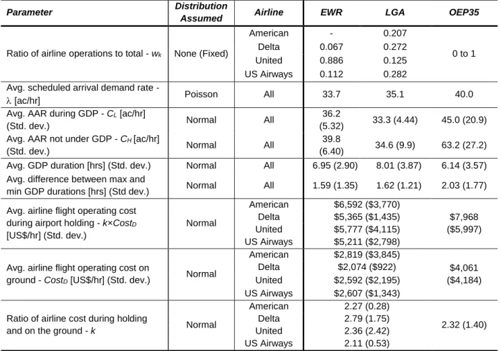
In order to gain a better understanding of how effective the approaches described in Section 3 are in setting system-wide performance goals, each approach is simulated, first for a generic TMI, and then for a specific TMI, a Ground Delay Program (GDP), at each of EWR and LGA airports. This allows us to derive general results, which cover various types of initiatives, and specific results, which provide an indication of likely results for a real-world case. In order to simplify the analysis, trade-offs are simulated between only two performance criteria, for a small number of airlines (between 3 and 4). This small number of airlines is reasonable given that the number of airlines with greater than 5% of operations at EWR and LGA, two of the busiest airports in the U.S., is 3 and 4, respectively (FAA, 2012). The forms of the trade space, Pareto frontier and airline payoff functions are described for each initiative in the following sections, followed by a description of the simulation methodology.
5.1 Generic Traffic Management Initiative
Trade Space and Pareto FrontierFor a generic TMI, we define a convex trade space, with the Pareto frontier defined by one of three alternative functions: an arc, a parabola, and a piecewise-linear function. The functional form of each of these is shown below as a function of G1 and G2, performance goals for two performance criteria (e.g.,
18
1. An arc: G12 + G22 = 1 (16)
2. A parabola: G2 = aG12 + bG1 + c, (17)
where a = –1 / (G1TP – 1)2; b = –2aG1TP; and c = –a – b.
G1TP represents the value of performance goal 1 at the turning point of the parabola, sampled from a uniform
distribution between 0 and 1. Defining the parabola in this way results in a Pareto frontier that more closely resembles the Pareto frontiers in the more realistic GDP scenarios described below. Note that only the right half of the parabola forms the Pareto frontier. The upper portion from the turning point to the G2 axis is
formed by a horizontal straight line, as shown in Figure 6b.
3. A piecewise-linear function: G2 = -m1G1 + 1, and (18)
G2 = -m2G1 + m2 (19)
m1 is sampled from a uniform distribution between 0 and 1, while m2 is sampled from a uniform distribution
between 1 and ∞. In our experiments, the Pareto frontier is described by only two lines, as shown in Figure 6c. In theory, any number of lines can be used.
(a) (b) (c)
Figure 6. Alternative Pareto frontiers describing the trade space for the generic TMI: a) an arc, b) a parabola, and c) a piecewise-linear function.
Airline Payoff Functions
The airline payoff functions are defined by concave increasing functions in these performance goals, rather than linear functions, because of the small buffers and redundancies built into airline schedules to reduce the impact of performance goal reductions of smaller magnitudes. Beyond a certain threshold, decreases in, e.g., capacity, lead to faster than linear increases in passenger re-accommodation costs, crew delay and reserve crew costs, airline recovery costs, etc. For the generic TMI, the payoff function for airline k is defined as the sum of quadratic functions of each of the two performance goals G1 and G2, as follows.
Pk = ∑ (𝑎𝑔,𝑘(𝐺𝑔∗) 2
+ 𝑏𝑔,𝑘
𝑔 (𝐺𝑔∗) + 𝑐𝑔,𝑘), ∀𝑘 (20)
19
The linear case is a special case of this function setting all 𝑎𝑔,𝑘 values to 0. Note that the additive constant
𝑐𝑔,𝑘 is later dropped from this expression without any loss of generality because it is inconsequential to any
of the analysis. The parameters defining each airline’s payoff function, ag,k and bg,k, are sampled from
uniform distributions from -1 to 0 (in the case of ag,k) and from 0 to 2 (in the case of bg,k, ensuring that bg,k >
-2ag,kso that the payoff is non-decreasing in each performance goal). It is noted that payoff functions do not
in fact need to be additive functions of G*g, and may include coupling between different performance goals.
The simpler additive function is, however, retained for this paper.
5.2 Ground Delay Program
Trade Space and Pareto FrontierFor the specific TMI, we consider a GDP under capacity uncertainty, in which we trade-off capacity and predictability. As described earlier, a GDP typically has three decision variables: duration, scope and magnitude. We apply two different models of a GDP. In the first, a simplified, computationally efficient model is applied in which we consider only duration, while in the second, we apply a more detailed model and consider both GDP duration and magnitude. In all cases we ignore the impact of GDP modification in response to updated information. The first model is run using Monte-Carlo methods, making use of the expressions for the expected values of capacity and predictability metrics developed by Liu and Hansen (2012). The second model is run for two specific GDP scenarios, one at each of EWR and LGA respectively, making use of expressions for the capacity and predictability metrics described in Appendix C. In the absence of closed form expressions for their expected values, we resort to numerical integration. A detailed Monte-Carlo simulation of the second model is not within the scope of this paper, but is considered a useful next step in this research. The second model should be treated as an example of how our modeling framework is easily extendable to more complex forms of ATM initiatives and its results further validate our main conclusions, as shown later in Section 5.
For the simplified model of the GDP, we utilize metrics for capacity and predictability derived for a single airport by Liu and Hansen (2012), assuming a constant scheduled arrival demand rate, λ. When the GDP is initiated, the AAR is reduced from a known constant high level, CH, which is assumed to be greater than λ, to
a known constant low level, CL, which is lower than λ. The planned duration of the GDP is T, at which time
the AAR is expected to return to CH. However, due to errors in prediction, the AAR may return to CH at a
different time, τ. When the GDP is initiated, T is set but τ is unknown, and assumed to be uniformly distributed between tmin and tmax. Conceptually, if T is set close to tmin, τis likely to be larger than T, and the
GDP ends late. In this case, capacity will be more fully utilized but there will be less predictability. Alternatively, if T is set close to tmax, then τis likely to be smaller than T, and the GDP ends early. In this
case, capacity will be underutilized and unnecessary delay will result. However, the delay is predictable. Thus, for this specific TMI, the only input from the airline is T, the planned duration of the GDP. Mathematical representations for capacity utilization and predictability, as developed by Liu and Hansen (2012), are presented below.
20
Capacity Utilization, αc, is defined as the ratio of realized throughput, from the beginning of the GDP until
the time when there is no more delay, to the maximum possible throughput with perfect information, were the airlines able to take advantage of the increase in AAR at time τ. αc varies from 0 to 1, and is shown by
Liu and Hansen (2012) to have the expected value shown below, which we use to define our metric for the performance goal of capacity Gc:
𝐺𝑐 = 𝐸[𝛼𝑐] = 𝑡𝑚𝑎𝑥−𝑇 𝑡𝑚𝑎𝑥−𝑡𝑚𝑖𝑛+ 𝑎 𝑐 ⁄ 𝑡𝑚𝑎𝑥−𝑡𝑚𝑖𝑛∙ 𝑙𝑜𝑔 ( 𝐵+𝑐𝑇 𝑏+𝑐𝑡𝑚𝑖𝑛), (21) where a = 𝜆𝐶𝐻−𝐶𝐿 𝐶𝐻−𝜆 𝑇 , 𝑏 = 𝐶𝐻 𝐶𝐻−𝐶𝐿 𝐶𝐻−𝜆 𝑇, and 𝑐 = 𝐶𝐿− 𝐶𝐻.
Predictability, αp, is defined as the ratio of expected flight delay, assuming the GDP ends at the planned time
T, to the total realized delay, i.e., the delay actually incurred given the early or late increase in AAR at τ.
Again, αp varies from 0 to 1 (given that we ignore GDP modifications in response to updated information),
and is shown by Liu and Hansen (2012) to have the expected value shown below, which we use to define our metric for the performance goal of predictability Gp:
𝐺𝑝= 𝐸[𝛼𝑝] = 1
𝑡𝑚𝑎𝑥−𝑡𝑚𝑖𝑛∙ (−
𝑇2
𝑡𝑚𝑎𝑥+ 2𝑇 − 𝑡𝑚𝑖𝑛). (22)
For the more detailed model of a GDP, we calculate expected values of the metrics for capacity and predictability through numerical integration for a single airport using a similar approach to that used by Liu and Hansen (2012), but allowing for a varying scheduled arrival demand rate λ(t), and planned and actual values of GDP AAR equal to CL and Cl, respectively. When the GDP is initiated, a planned AAR, CL, is
specified, which is lower than λ. This represents the expected AAR for the duration of the GDP. As in the simplified model, the planned duration of the GDP is T, at which time the airport capacity is expected to return to the known CH, which is greater than λ. Due to errors in prediction, the actual AAR (Cl) for the GDP
may be different than that planned. Similarly, the AAR returns to CH at a time τ, which may be different than
that planned. When the GDP is initiated, CL and T are set but Cl and τ are unknown. They are assumed to be
uniformly distributed between CL min and CL max, and tmin and tmax, respectively. Conceptually, if CL is set close
to CL min, Clis likely to be larger than CL, and the rate at which aircraft arrive at the airport will be lower than
the available capacity. In this case, capacity will be underutilized and unnecessary delay will result. However, the delay is predictable. Alternatively, if CL is set close to CL max, then Clis likely to be smaller
than CL, and arriving aircraft will be required to hold because they will arrive at a faster rate than the airport
can accommodate. In this case, the available capacity will be more fully utilized but there will be less predictability. As in the simplified model, if T is set close to tmin, τis likely to be larger than T, and the GDP
ends late. In this case, capacity will be more fully utilized but there will be less predictability. Alternatively, if T is set close to tmax, then τis likely to be smaller than T, and the GDP ends early. In this case, capacity will
be underutilized but predictability will be high.
As in the simplified model, Capacity Utilization, αc, is defined as the ratio of realized throughput, from the
beginning of the GDP until the time when there is no more delay, to the maximum possible throughput with perfect information, were the airlines able to take advantage of the actual GDP AAR Cl, and the increase in
AAR at time τ. The value of αc varies from 0 to 1. Predictability, αp, is defined as the ratio of expected flight
delay, assuming the planned GDP AAR CL and the planned GDP end time T, to the total realized delay, i.e.,
21
the value of αp varies from 0 to 1 (given that we ignore GDP modifications in response to updated
information). Expressions for αc and αp are presented in Appendix C. Based on these expressions, the
expected value of the performance goals for capacity Gc and predictability Gp, can be calculated through
numerical integration assuming uniform distributions of Cl between CL min and CL max, and τ between tmin and
tmax. For numerical integration, we divide the range of possible values of Cl into 60 discrete points (steps of
0.1 aircraft/hour, across 6 aircraft/hour) and the range of possible values of τ into 60 discrete points (steps of 2 minutes, across 2 hours).
Given the specification of performance goals for capacity and predictability, the trade space is identified by calculating Gc and Gp across the range of planned CL values from CL min to CL max, and T values from tmin and
tmax, using data from the FAA Aviation Systems Performance Metrics (ASPM) database (FAA, 2012) and
GDP duration data made available by Metron Aviation®, described in detail in Section 5.3 below. The Pareto
frontier is then identified for this trade space by discretizing the range of Gp values into a set number of
points (100), and extracting the maximum corresponding value of Gc in each case. The relationship between
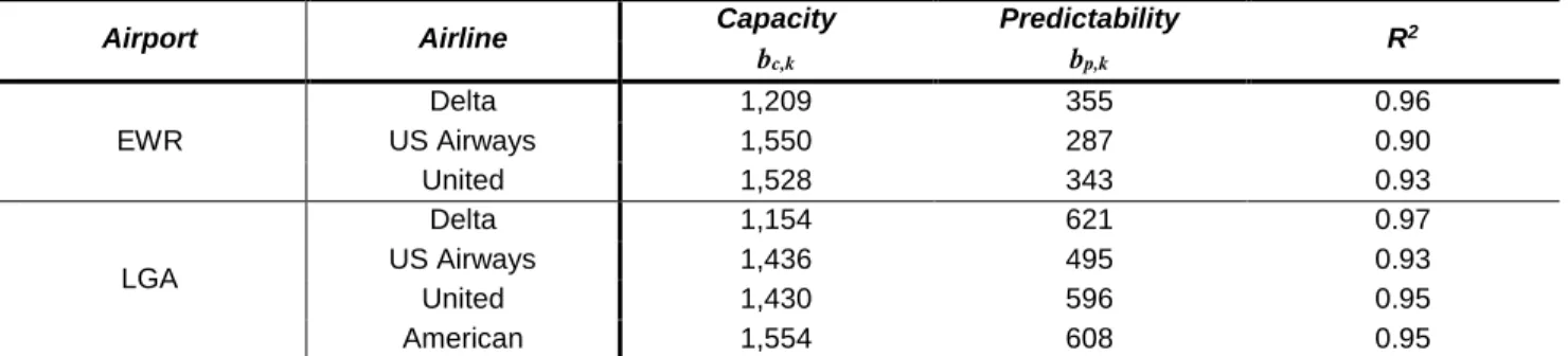
the capacity and predictability metrics on the Pareto frontier was found to be very close to parabolic. A parabolic function is therefore fitted to the resulting maximum values of Gc for each given value of Gp, of the
form:
Gc = aGp2 + bGp + c (23)
We used the aforementioned 100 points on the Pareto frontier to estimate 3 parameter values (a, b, and c). Note that this model described in equation (23) is linear in parameters and hence the parameters can be estimated using an ordinary least squares (OLS) estimator. The estimation was performed using the standard
MATLAB function for linear regression. Using data from the ASPM database (FAA, 2012), Form 41
database (DOT, 2012), and GDP duration data made available by Metron Aviation®, described in detail in
Section 5.3, the estimated parameters and fit performance at EWR and LGA are shown in Table 1. The parabolic nature of the relationship is confirmed by the consistently highR2 values shown.
Airport a b c R2
EWR -0.485 0.663 0.776 0.91
LGA -1.086 1.626 0.395 0.93
Table 1. Estimated Pareto frontier parameters for the detailed GDP model
Airline Payoff Functions
For the simplified GDP model, airline payoff functions are defined based on the cost of the flight delays incurred as a result of the GDP (payoff is therefore negative), similar to the way in which Liu and Hansen (2012) define a metric for efficiency. We assume that all the flights depart their respective origin airports under the assumption that the GDP ends at exactly the planned GDP end time T. If the actual GDP end time,
τ, is before or equal to T, flights incur a delay on the ground equal to the difference between the actual
departure time based on the planned GDP end time and the originally scheduled departure time. We assume that this delay is incurred at a specific ground delay cost of CostD dollars/minute, which varies by airline. If,