HAL Id: hal-01322875
https://hal.archives-ouvertes.fr/hal-01322875
Submitted on 28 May 2016
HAL is a multi-disciplinary open access archive for the deposit and dissemination of sci-entific research documents, whether they are pub-lished or not. The documents may come from
L’archive ouverte pluridisciplinaire HAL, est destinée au dépôt et à la diffusion de documents scientifiques de niveau recherche, publiés ou non, émanant des établissements d’enseignement et de
Projecting and valuing domestic water use at regional
scale: A generic method applied to the Mediterranean
at the 2060 horizon
Noémie Neverre, Patrice Dumas
To cite this version:
Noémie Neverre, Patrice Dumas. Projecting and valuing domestic water use at regional scale: A generic method applied to the Mediterranean at the 2060 horizon. Water Resources and Economics, Elsevier, 2015, 11, �10.1016/j.wre.2015.06.001�. �hal-01322875�
Projecting and valuing domestic water use at regional
scale: a generic method applied to the Mediterranean at
the 2060 horizon
No´emie Neverrea,b,d,∗, Patrice Dumasa,c
a
Centre International de Recherche sur l’Environnement et le D´eveloppement (CIRED), Campus du Jardin Tropical, 45 bis avenue de la Belle Gabrielle, 94736 Nogent sur
Marne, France, b
Centre National de la Recherche Scientifique (CNRS), 3 rue Michel-Ange, 75016 Paris, France
c
Centre de coop´eration Internationale en Recherche Agronomique pour le D´eveloppement (CIRAD), 42 rue Scheffer, 75016 Paris, France
d
Ecole Nationale des Ponts et Chauss´ees (ENPC), Cit´e Descartes, 6-8 avenue Blaise Pascal, 77455 Champs-sur-Marne, France
Abstract
The present work focuses on the demand side of future water scarcity assessment, and more precisely on domestic water demand. It proposes a quantitative projection of domestic water demand, combined with an origi-nal estimation of the economic benefit of water at large scale. The general method consists of building economic demand functions taking into account the impact of the level of equipment, proxied by economic development. The cost and price of water are assumed to grow with economic development.
The methodology was applied to the Mediterranean region, at the 2060 horizon. Our results show the evolution of water demand and value, mea-sured by surplus, over time. As long as GDP per capita and water price remain low, demand per capita increases along with economic development, and surplus per capita increases with demand. As demand approaches sat-uration, the combined negative effects of water cost and price increase on surplus grow stronger, and surplus per capita begins to decrease.
The developed methodology is meant to be used for large-scale hydroe-conomic modelling, in particular for regions with heterogeneous levels of development and low data-availability.
Keywords: Domestic water demand, Water value, Projection, Hydroeconomic modeling, Mediterranean
∗
corresponding author
Email addresses: neverre@centre-cired.fr (No´emie Neverre), dumas@centre-cired.fr (Patrice Dumas)
1. Introduction
Pressure on water resources is a major issue in the Mediterranean region. More than half of the world’s “water-poor” population is located in the re-gion, which concentrates 7.3% of the world’s population for only 3% of its water resources [25]. Global changes are expected to exacerbate this pres-sure on resources in the following decades: on the one hand water demand will increase with demographic growth and economic development, while on the other hand climate change is predicted to reduce water availability and intensify droughts around the Mediterranean [7].
Spatially contrasted situations, with some basins more affected by water scarcity than others, could foster water related interactions between basins such as water transfers, activity relocations and, indirectly, migrations. Such interactions could particularly arise in the case of the Mediterranean, which has a history of exchanges and migrations between rims [9].
In such a context, it is important to anticipate future water scarcity issues and identify basins at risk, in order to inform management strategies and policies. Traditionally, water management policies focused on adapting supply to demand, by mobilizing new water resources. But as resources become increasingly scarce and costly, policy makers have developed demand side management aiming at reducing water wastage.
In the present work we concentrate on the demand side of the water scarcity issue, and more precisely on domestic water demand. Irrigation is the largest water use sector in the Mediterranean, representing 63% of total water use [25], and its projection is a research field of interest [10]. However, its share in total water use is decreasing [25]. Moreover, domestic demand, while accounting for a lower share of demand, is critical in terms of needs. Indeed, irrigation needs can be adjusted to some extent by virtual water trade, water scarce areas having the possibility of importing food rather than producing it themselves [4]. Domestic needs cannot be adjusted in that way. In addition, domestic uses such as consumption, food preparation and hygiene are essential to human life.
Some projections of domestic water use in Mediterranean countries exist, but they are not homogeneous between countries in terms of time horizons, methods and scenarios. In most cases they rely on simple trend prolonga-tions [25]. When looking at the whole region, a global projection method-ology applicable to the different countries, taking into account sociodemo-graphic changes to come and simulating comparable scenarios across coun-tries is pertinent.
Generic global scale modelling of domestic water use is covered exten-sively in the literature [2, 3, 36, 17, 37]. The general principle is to model and project a unitary water use intensity per capita, that is to be multiplied by the projected number of inhabitants. In the WaterGAP methodology [1], the per capita water use intensity is modelled to evolve with the level of economic
development (relationship statistically estimated at country scale) and de-crease over time with technological improvement (represented by a fixed rate of improvement). In the Total Runoff Integrating Pathways (TRIP) model, future levels of domestic water use per capita in developing countries have been modelled either to converge towards that of present developed countries as economic growth continues [36, 19], or independently from eco-nomic growth [17]. Other authors consider the impact of additional factors: Hughes et al. [21] statistically estimate municipal water use per capita as a function of climatic variables and GDP per capita; Ward et al. [37] estimate municipal water demand as a function of GDP per capita and urbanisation rate, taking into account regional dummies and country characteristics as fixed effects.
While evaluating water quantities at stake is essential, it is also relevant to have an idea of the economic benefits associated with water uses and the potential economic losses associated with water shortage. Economic valua-tion can be an indicavalua-tion on how to manage at best the available resource and allocate it between competitive uses when water is scarce. In hydroeco-nomic models, instead of considering water demands as fixed requirements, water is allocated to its different uses based on the economic benefits it gen-erates: the economically optimal allocation is the one that maximises the aggregated economic value of the water used [18].
However, economic valuation of domestic water, as well as methods to project changes in water value, are absent from the large-scale literature. Because markets are absent or inefficient for the water sector, it is not pos-sible to observe directly the economic value of water. It is necessary to develop alternative non-market valuation techniques to reveal and estimate water’s value [39]. For the domestic sector, water is valued using willingness to pay and deriving economic surplus from econometric estimations of price-elasticity and demand functions [39]. Such a method requires much data, which could be among the reasons explaining why hydroeconomic models have been developed mainly at an infra-national geographical scale [18].
To account for changes in both demands and economic benefits, in a region with heterogeneous data-availability, we develop an original generic method. We build an economic demand function, analogous to the demand function modelling approach used in hydroeconomic models of smaller scale [30], which enables water valuation. In order to take into account the link between water use and economic development, a methodology similar to WaterGap [1] is used.
This paper first describes the methodology developed to build generic demand functions that project both quantities and economic values of future domestic water demands at large scale and at a time horizon enabling to picture global changes (Cf. diagram in AppendixA). Then it proposes an application to countries of the Mediterranean rim, from Western and Eastern Europe, Middle East and North Africa (Cf. map of Mediterranean countries
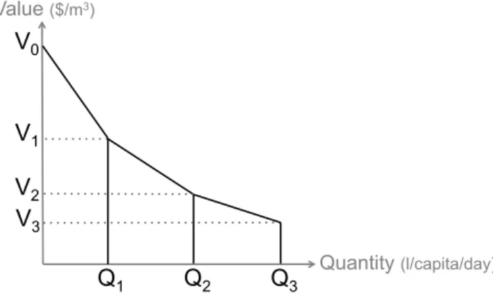
V2 V0 Q1 Q2 Q3 Value ($/m3) Quantity (l/capita/day) V3 V1
Figure 1: General structure of the three-part inverse demand function (with volumes Q and willingness to pay V )
in AppendixB).
2. Building generic demand functions taking into account struc-tural change
2.1. Overview
Our approach is to build simple three-part inverse demand functions (Figure 1), in which the willingness to pay for water decreases with quantity [18]. Each part of the demand function corresponds to a different cate-gory of use. The first catecate-gory corresponds to basic water requirements for consumption, food and hygiene, which are very highly valued (e.g. hand washing). The second category corresponds to intermediate needs, including additional hygiene (regular laundry, showers etc.), less valued than uses of the first category. The last category corresponds to least-valued supplemen-tary consumption, such as further indoor uses (e.g. leisure bath) or outdoor uses (lawn watering, pool, fountain etc.).
To build a demand function for each country, we determine the bounds of the demand blocks corresponding to these three categories: their respective volume limits (noted Q) and the marginal willingness to pay (noted V ) for those volumes.
Hence, the first step of the methodology is to determine the volume limits of the demand blocks, taking into account that demand will be impacted by economic development processes. The second step is to determine the willingness to pay for water at those volumes of reference, in order to value water. This second step also makes it possible to take into account the possible impact of water price on demand.
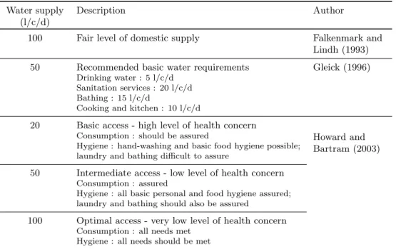
Table 1: Domestic water supply levels of reference, in litres per capita per day (l/c/d). The figures 50 l/c/d and 100 l/c/d are used in the demand function.
Water supply (l/c/d)
Description Author
100 Fair level of domestic supply Falkenmark and
Lindh (1993)
50 Recommended basic water requirements
Drinking water : 5 l/c/d Sanitation services : 20 l/c/d Bathing : 15 l/c/d
Cooking and kitchen : 10 l/c/d
Gleick (1996)
20 Basic access - high level of health concern
Consumption : should be assured
Hygiene : hand-washing and basic food hygiene possible; laundry and bathing difficult to assure
Howard and Bartram (2003) 50 Intermediate access - low level of health concern
Consumption : assured
Hygiene : all basic personal and food hygiene assured; laundry and bathing should also be assured
100 Optimal access - very low level of health concern
Consumption : all needs met Hygiene : all needs should be met
2.2. Volumes of the demand blocks: taking into account structural change Following Alcamo et al. [1] and their “structural change” modelling, we want to take into account that average domestic water demand per capita grows along with economic development, proxied by GDP per capita, in or-der to take into account equipment effects. Indeed, as their income increases households get more water-using appliances (washing machines, dishwasher etc.) and use more water; eventually they reach equipment saturation and water use stabilizes whilst income continues to grow. To take into account structural change, we consider that the volumes of the blocks of our demand function evolve over time following economic development.
We assume that only non-essential uses are sensitive to this equipment effect, so we consider that the volume of the first block of our demand function is fixed. Following Gleick [16] and Howard and Bartram [20] (Table 1), we set the volume limit of the first demand block to 50 litres per capita per day, which meets needs for consumption, food and personal hygiene.
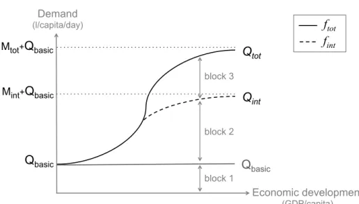
The volumes of the second and third demand blocks are assumed to evolve with the level of GDP per capita, with a saturation, drawing a sigmoid curve (Figure 2). When GDP per capita is low, water demand is composed of only basic uses and intermediate uses (categories 1 and 2); intermediate uses grow with economic development. Then, as GDP per capita further increases, third category uses appear and the third demand block grows
Qbasic Demand (l/capita/day) block 3 block 2 block 1 Qtot Qint Economic development (GDP/capita) Mtot+Qbasic Mint+Qbasic Qbasic ftot fint
Figure 2: Evolution of domestic water demand with economic development: “structural change” modelling (with volumes Qbasic, Qint and Qtot)
along with the intermediate demand block. Eventually, demand reaches saturation and stabilizes.
To determine the total demand (Qtot) structural change curve, we use
the sigmoid function ftot:
Qtot= ftot(GDP ) = mtot+ Mtot.[1 − exp(−γtot.GDP2)]
The function ftot is defined by three parameters: the minimum demand
(mtot), the maximum additional demand (Mtot) and the curve parameter
(γtot); GDP stands for average GDP per capita. Parameter mtot is set to
match basic needs: mtot = Qbasic= 50 l/c/d. The two remaining
param-eters of ftot are to be statistically estimated at country scale using GDP,
population and domestic water demand data (Section 3.1).
Then, to distinguish between second-block and third-block volumes, we introduce the following sigmoid curve fint:
fint(GDP ) = mint+ Mint.[1 − exp(−γint.GDP2)]
This curve fint is defined only starting from its intersection with ftot, noted
(GDP°, Q°). Before this wealth level GDP°, demand of the third category is null; after, intermediate demand is: Qint = fint(GDP ), and demand of
the third category is: Qtot− Qint(Figure 2).
Parameters of fint are completely determined without need for a
sta-tistical estimation. First, we set: mint= Qbasic= 50 l/c/d. Then Mint is
set so as to match the reference figures of a “fair level of domestic supply” from the literature [12, 20]: Mint+ mint= 100 l/c/d (Table 1). Finally, we
constrain fintby setting its inflection point so as to belong to the curve ftot,
which determines γint.
Once structural change curves parameters are calibrated for a chosen country, the volumes of the blocks of its demand function can be determined for a given year depending on the level of GDP per capita (Figure 2). 2.3. Willingness to pay for water along the demand function
Once the volumes of water demand are determined, we estimate the will-ingness to pay (WTP) for water along the demand function. The following section describes how we determine the WTP at the lower and upper bound volumes of each category (i.e. 1st, 50th and 100th l/c/d, and maximum po-tential demand), then interpolate linearly.
We collected econometric studies, located in the Mediterranean region or in Europe, that estimate the response of domestic water demand to price. Studies that provided both estimated price elasticities and observed levels of price and demand were used to calculate the marginal willingness to pay for water along the demand curve for each study, following the point-expansion method [18]. Demand values were adjusted for some studies [6, 14, 15, 28, 29, 27] to include collective uses, based on the assumption that collective uses represent 25% of total municipal uses, the remainder corresponding to residential uses. For one of the studies [31] the number of persons per household was assumed to be 2.57, which was the average 1990 household size in France at the time of the study (data from the French National Institute of Statistics and Economic Studies).
Some studies [6, 28, 29, 27] displayed very low prices (0.49 to 0.86 $2005/m3), associated with very low demands (104 to 157 l/c/d). One study
[15] on the contrary displayed a very high demand (369 l/c/d) for a higher price (1.64 $2005/m3). Some studies performed the econometric estimation
with a linear structural form [15, 28, 29, 27] , others with a log-log structural form (i.e. constant price-elasticity) [6, 14, 31, 35]. The linear studies led to low slopes, with a very low WTP for water for the first litre consumed (1.59 to 4.98 $/m3), and WTP in the [0.57 $/m3; 4.09 $/m3] range for the 100th
l/c/d [15, 28, 29, 27].
For low demand levels, the linear structural forms are likely to under-estimate water values since under-estimates are much lower than prices actually paid for (e.g. bottled water, which can reach 300 $/m3 or higher). More-over, such low values do not agree with the notion that water is essential [5]. Values given by log-log structural forms are higher, but the econometric esti-mations were performed in conditions where observed demands were higher than 100 l/c/d. For low demand levels, i.e. the 1st and 50th l/c/d, which are far from the observations range of the estimations, we chose not to rely on econometric estimates of WTP for water and made simple assumptions (Table 3).
0
50
100
150
200
250
300
350
Volume (l/capita/day)
0
2
4
6
8
10
12
14
16
18
Wi
llin
gn
ess
to
pa
y (
$
2005/m
3)
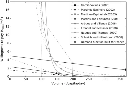
Garcia-Valinas (2005) Martinez-Espineira (2002) Martinez-EspineiraME2003) Martins and Fortunato (2005) Arbues and Villanua (2006) Frondel and Messner (2008) Nauges and Thomas (2000) Schleich and Hillenbrand (2008) Demand function built for FranceFigure 3: Marginal willingness to pay along the demand curve, calculated from the results of various econometric studies. In grey: econometric es-timations using a log-log structural form, in black: linear structural form. Markers indicate the average observed levels of demand and price for each study. The dotted curve represents the demand function built for France, the pentagonal marker indicates the point of maximum potential demand calibrated for France and current water price in France.
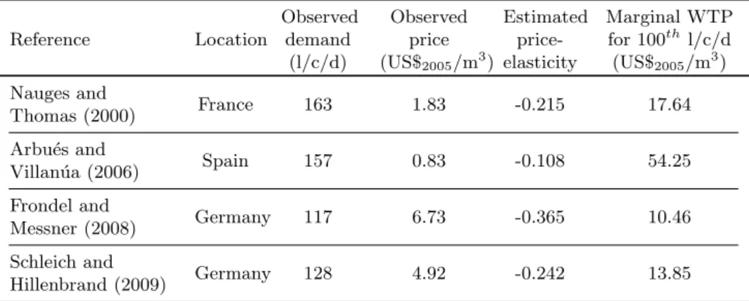
For the 100thl/c/d, values given by the linear form are much lower than values obtained with log-log structural form. Even though there is no strong evidence that the values given by the linear form are incorrect, we assumed that values were too low at this demand level. Therefore, we chose to rely only on the marginal WTP for water calculated from studies using a log-log structural form. Three studies remained, after we chose not to use the results derived from Arbu´es and Villan´ua [6], for which a high observed demand combined with a low price-elasticity imply a steeper slope and much higher values than the other studies (Figure 3 and Table 2). Demand consists of total domestic demand (i.e. residential uses and collective uses).
The marginal WTP for the 100thl/c/d ranges from 10.46 to 17.64$/m3,
with a 25% variation range around the average of 14. We assume that
the WTP for the 100th l/c/d is 14 $/m3. Because the error range of this parameter is high, it is included in the sensitivity analysis performed in Section 4.
Table 2: Marginal willingness to pay (WTP) for the 100th litre per capita per day (l/c/d), calculated from the results of four econometric studies
Reference Location Observed demand (l/c/d) Observed price (US$2005/m3) Estimated price-elasticity Marginal WTP for 100thl/c/d (US$2005/m3) Nauges and Thomas (2000) France 163 1.83 -0.215 17.64 Arbu´es and Villan´ua (2006) Spain 157 0.83 -0.108 54.25 Frondel and Messner (2008) Germany 117 6.73 -0.365 10.46 Schleich and Hillenbrand (2009) Germany 128 4.92 -0.242 13.85
For the upper bound of the third block, we use available data on cur-rent water price. Combining observed quantity and observed price could give us a point of the demand curve. However, if equipment limits demand, there is some rationing and the point of observed demand does not corre-spond to the consumption level where willingness to pay equals price and consumer’s marginal surplus becomes null. To estimate this level of de-mand, unconstrained by equipment, we use the maximum potential demand Qbasic+Mtot, i.e. the plateau of the structural change function ftot. Hence we
use Qbasic+ Mtot and Pt=0 as a reference point of the demand curve, where
Pt=0 is the current water price, determined by the authors from available
data (Table 5 and Section 3.2). This point constitutes the upper bound of the third category demand block (Table 3). Then, for a given year, the third block actually ends when reaching Qtot, i.e. the actual total demand for the
level of GDP per capita of the considered year, as demand is constrained by revenue and domestic equipment (Figure 4).
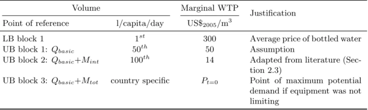
Table 3 summarises the figures used to define the WTP for water at the bounds of the blocks of our three-part inverse demand function. Once the WTP for water at the volume points of reference of the three categories of demand has been determined, a linear interpolation is used to build the demand function. The linear form is chosen for its simplicity, in absence of data justifying another shape.
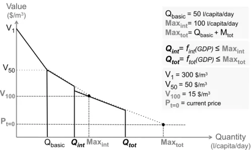
In this way, we build a domestic demand function for each country, whose parameters take into account the impact of economic development on demand. The structure of that final demand function is pictured in Figure 4, where Qintand Qtot are being redetermined for each year following projected
GDP per capita. The total economic value of the water used can be derived from this demand function, depending on the cost of water, the price of water and the level of satisfaction of the demand: it consists of consumers’
Table 3: Marginal willingness to pay (WTP) at the bounds of the blocks of the three-parts demand function, with LB: lower bound, UB: upper bound.
Volume Marginal WTP
Justification
Point of reference l/capita/day US$2005/m3
LB block 1 1st 300 Average price of bottled water
UB block 1: Qbasic 50th 50 Assumption
UB block 2: Qbasic+Mint 100th 14 Adapted from literature
(Sec-tion 2.3)
UB block 3: Qbasic+Mtot country specific Pt=0 Point of maximum potential
demand if equipment was not limiting
Table 4: Calibrated maximum potential demand for the different countries (where m3/c/y: cubic metre per capita per year; and l/c/d: litre per capita per day)
Country Mtotparameter Maximum potential demand Willmott index
of agreement (m3/c/y) (m3/c/y) (l/c/d) France 54.52 72.77 199 0.00 Israel 71.79 90.04 247 0.41 Italy 92.11 110.36 302 0.63 Malta 54.49 72.74 199 0.65 Slovenia 82.08 100.33 275 0.44 Spain 91.26 109.51 300 0.83 Othersa 77.58 95.83 263 -a
Albania, Algeria, Bosnia, Croatia, Cyprus, Egypt, Greece, Lebanon, Libya, Morocco, Syria, Tunisia, Turkey, Montenegro
V100 Pt=0
Qbasic Qint Qtot Maxtot V50 Value ($/m3) Quantity (l/capita/day) Maxint Qbasic = 50 l/capita/day Maxint= 100 l/capita/day Maxtot= Qbasic+ Mtot Qint= fint(GDP) ≤ Maxint
Qtot= ftot(GDP) ≤ Maxtot V1 = 300 $/m3
V50= 50 $/m3 V100 = 15 $/m3 Pt=0 = current price V1
Figure 4: Structure of the final three-parts inverse demand function and its points of reference (volumes Q and values V ). Qbasicis set to 50 l/capita/day,
whereas Qint and Qtot depend on the level of GDP per capita on the
con-sidered year. Qint and Qtot grow with GDP per capita with a saturation,
their maximum value are respectively M axint and M axtot. M axintis set to
100 l/capita/day, whereas M axtot is calibrated at country scale.
surplus plus the water utility’s revenue (AppendixC). Water utility’s revenue can be negative if price is lower than cost.
A sensitivity analysis is later carried out to assess the impact of the different assumptions (Section 4).
3. Application to the Mediterranean region
The first step is to calibrate structural change curves for each country. Then, for a given year t and level of GDP per capita GDPt, potential
in-termediate and total demands can be determined and used to define the volumes of the blocks of the three-part demand function for year t (Figure 4). Finally, actual demand for year t can be determined depending on the price of water Pt.
3.1. Calibration of structural change curves for the Mediterranean countries Structural change curves parameters (M and γ, Cf. Section 2.2) were calibrated for countries of the Mediterranean rim based on data available at a regional scale. Historical water demands were determined using water withdrawal data at country level from the Mediterranean Information Sys-tem on Environment and Development database (SIMEDD [33]) and water withdrawal to water demand ratios (i.e. water networks’ efficiency) from
Margat and Treyer [25]. Population data were taken from UNO, GDP data from World Bank. All GDP figures are expressed in purchasing power parity terms, in US$2005.
Data was available to calibrate the structural change curves for six coun-tries (France, Italy, Israel, Malta, Slovenia, Spain). For the other councoun-tries, historical GDP per capita is low and data is concentrated in the lower part of the sigmoid, so the plateau of the curve cannot be estimated. In such case, assumptions based on available data and assumptions on country sim-ilarities1 need to be made. For Montenegro, we used the plateau calibrated on Greece. For the remaining countries, in absence of a suitable country of reference, we set the maximum additional demand parameter (Mtot) and
pricing (Pt=0) to the average value in countries where it could be estimated,
and calibrated only the curve parameter (γtot). For Montenegro, we did not
have sufficient data to fit the curve parameter either, so we used the curve parameter calibrated on Greece.
Results of the calibration of the Mtot parameter and resulting
maxi-mum potential demands for each country are presented in Table 4. The plateau level is the lowest in Malta and France, and the highest in Spain and Italy. Goodness of fit between country data and the obtained calibrated function is evaluated with Willmott index of agreement in its original form [38], which is suitable for sigmoid curves. For France, the curve fits well visually (AppendixD), but in this specific case the Willmott index is not an appropriate indicator of goodness of fit because historical consumption has already reached the plateau and observations are flat (instead of being of a sigmoid form), so the sum of squares of the regression (SSR) is null.
In our methodology the projection variable is demand, leaving the pos-sibility of making various assumptions about the evolution of network ef-ficiency when determining the corresponding withdrawal. To be able to compare our calibration results with those of the WaterGAP methodology applied to European countries [13], we converted our demand figures into withdrawals under the assumption that demand to withdrawal ratios re-main equal to current ratios (average current ratios, adapted from Margat and Treyer [25], Cf. Table 6). For Spain and Slovenia, our results are very similar to Fl¨orke and Alcamo [13] findings, with less than 10% of difference in maximum potential withdrawals, whereas for France and Italy we obtain substantially lower results (-65 to -85%). Fl¨orke and Alcamo [13] perform their structural change calibration using adjusted data: they offset past im-provements in water use efficiency by applying a fixed annual technological change rate. The adjusted data they use are therefore higher than historical data, which can explain the differences with our results for France and Italy.
1Maximum potential demands should reflect cultural effects, along with other factors influencing domestic water demand (climate, household characteristics etc.).
For Malta, Fl¨orke and Alcamo [13] obtained a very low plateau (about two times lower than ours), which could be because their data do not take into account desalinated water.
3.2. Projection scenarios
The calibrated three-part demand curves were used for the projection and valuation of domestic water demands in the Mediterranean countries, as a function of economic development and water price. Since demands are mostly higher than the upper bound of the second block (100 l/capita/day), for simplification we used the average value of water per block instead of the variable marginal value in the first two blocks of the demand functions when calculating consumer’s surplus. This could lead to an underestimation of consumer’s surplus when demand is lower than 100 l/capita/day (Morocco before year 2010, Bosnia before 2015, Tunisia before 2020, Algeria until 2050 under the reference scenario).
Projection and valuation of future domestic water demands at the 2060 horizon were performed under contrasted scenarios of economic development and population growth. For economic development scenarios, we used GDP projections of the five Shared Socioeconomic Pathways (SSPs) [34] available in the SSP Database (version 0.9.3). For population projections, we used four UNO scenarios: the medium, low and high variants, and the constant fertility variant. The medium population variant combined with the SSP2 economic scenario is used as the reference scenario.
The cost of water was assumed to evolve over time as countries develop and invest in water infrastructures. Current cost level in France was chosen as a target cost of reference, because we consider it to be representative of a mature domestic water distribution and sewerage service, with a cost-recovery ratio close to one. We assume that, as far as conventional water resources are concerned, water costs mainly consist of distribution and sew-erage costs and do not differ greatly between countries (this assumption is relaxed in Section 3.4). Cost evolution was hence represented as follows: in every country water cost increases over time and converges towards the current cost level in France, following the evolution of GDP per capita. It is not allowed to decrease if GDP per capita drops. Water cost reaches the target cost level when GDP per capita reaches the current level of GDP per capita in France.
For Malta, the particular context of the water sector implies a very high cost of water due to intensive desalination: 62% of the water used came from desalination in 1998-1999 [25]. For Croatia, the current cost of water is also above the target cost level. Therefore, no further increase in water cost was projected for Malta and Croatia.
The cost-recovery ratio was assumed to converge towards one as GDP per capita grows, reaching one when GDP per capita reaches the current
level of GDP per capita in France. The price of water changes over time, resulting from the combination of cost evolution and cost-recovery evolution. Current water prices and costs in each country were not directly avail-able, they had to be reconstructed using available data on water costs or prices from Margat and Treyer [25], OECD [32] and International Bench-marking Network for Water and Sanitation Utilities database (IBNET [22]), cost-recovery ratios from Margat and Treyer [25], Euro-Mediterranean Wa-ter Information System database (EMWIS [11]) and IBNET, and sewerage coverage ratios from EMWIS and IBNET. Domestic water prices and costs are estimated with two different methods: using available data on prices and costs, or reconstructing costs based on the most robust data and sew-erage covsew-erage rates. Then the maximal value given by these two methods is selected, to avoid unrealistically low values.
For the first method, in a first step data on water prices and costs are deflated. When possible, missing costs are determined using the cost/price ratio in each country. If this information is not available, the water volumes weighted average Mediterranean cost/price ratio is used (using SIMEDD data for year 2000 water volumes). The obtained values are then multiplied by a 1.3 factor to take into account additional costs (other than operational costs). The 1.3 figure originates from data on France from Margat and Treyer [25]. Robust water costs data are available for four countries (France, Greece, Italy and Spain), the minimum estimated costs are observed for Italy (2.17$/m3). This minimum cost accounts for both water services and sanitation services, each representing 50% of this cost. We use this value as a basis to calculate minimum costs for all the other countries in the second method.
For the second method, we estimate a minimal domestic water cost de-pending on the sewerage coverage rate. For countries where robust water costs data are not available, we assume that water distribution services costs are 2.17/2 $/m3 (i.e. half of the minimum total cost among countries with robust data). We then add sanitation costs, which vary from 0 to 2.17/2 $/m3, depending on the sewerage coverage rate.
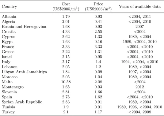
Final cost and price data used are displayed in Table 5. 3.3. Projection results
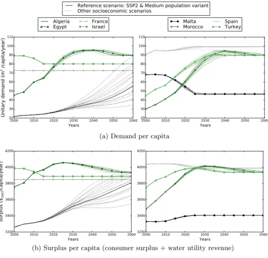
Results of projected water demand per capita are presented in Figure 5 for a selection of countries and in Table 6. Developed countries have mostly reached demand saturation: demand per capita does not increase in France, Israel and Malta, and it increases by only 2.1% to 9.7% in Spain between 2000 and 2060 under the different scenarios. In contrast, demand per capita grows sharply in developing countries, at a pace depending on socioeconomic drivers. In Egypt, domestic water demand per capita is of 45.36 m3/c/y in 2000, and it grows rapidly and reaches potential demand around 2030-2035 (Figure 5(a)). In Morocco and Algeria, initial demand
Table 5: Reconstructed current costs and prices of domestic water in Mediterranean countries (around year 2000)
Country Cost Price Years of available data
(US$2005/m3) (US$2005/m3)
Albania 1.79 0.93 <2004, 2011
Algeria 2.01 0.41 <2004, 2010
Bosnia and Herzegovina 1.68 0.93 2007
Croatia 4.33 2.55 <2004 Cyprus 2.62 1.33 1989, <2004 Egypt 1.63 0.16 1989, <2004, 2010 France 3.33 3.33 <2004, <2010 Greece 2.22 1.31 <2004, <2010 Israel 2.15 0.95 <2004, <2010 Italy 2.17 1.4 1994, <2004, <2010 Lebanon 2.05 1.2 1989, <2004
Libyan Arab Jamahiriya 1.84 0.09 1997, <2004
Morocco 2.05 1.04 1989, <2004
Malta 10.58 2.08 <2004
Montenegro 1.65 0.93 2012
Slovenia 2.81 1.66 <2004
Spain 2.75 1.62 <2004, <2010
Syrian Arab Republic 2.83 0.91 1989, <2004
Tunisia 1.9 0.91 1989, 1996, <2004, 2010
Turkey 2.1 1.17 <2004, 2008
is lower (respectively 29.97 and 21.70 m3/c/y in 2000); whereas it grows rapidly in Morocco, reaching potential demand around 2035-2040, it grows more slowly in Algeria where GDP per capita evolves at a slower pace, and maximum potential demand is not yet reached in 2060 under the reference scenario.
An overshoot effect is perceptible for Egypt and Morocco (Figure 5(a)) after 2040, as the growth of demand per capita is counterbalanced by in-creases in water price (with an order of magnitude of -6.3% in demand in 2060 due to price increase). This impact of price on demand is also visible for Israel and for Spain (respectively -10.9% and -8.9% in 2060).
While GDP per capita and water price remain low, demand per capita increases with economic development, and surplus per capita increases with demand. Eventually, when GDP per capita and price reach a certain level, demand per capita begins to saturate and decrease, which impacts surplus negatively. In parallel, as the country develops the cost of water increases, which also impacts surplus negatively. As a result, surplus per capita begins to decrease sooner than demand per capita. The negative net effect on surplus is visible for Egypt, Israel, Morocco, Spain and Turkey (Figure 5(b)). Malta is a particular case. The cost of water is the highest among Mediterranean countries: 10.58 $2005/m3 compared with an average cost
Table 6: Projected domestic demands in Mediterranean countries for years 2010, 2025 and 2050, for the reference socioeconomic scenario
Country
Total demand Demand per capita Demand to
withdrawal ratios (%)a (km3/y) (m3/c/y) 2010 2025 2050 2010 2025 2050 Albania 0.30 0.32 0.28 93.49 95.72 93.21 45 Algeria 0.83 1.22 2.03 23.52 29.04 43.57 50
Bosnia and Herzegovina 0.13 0.21 0.27 35.63 59.01 89.79 40
Croatia 0.31 0.35 0.33 69.97 83.3 84.73 67.5 Cyprus 0.07 0.08 0.12 61.54 64.57 86.39 77 Egypt 4.86 8.78 11.35 59.93 86.96 91.96 52.5 France 4.57 4.89 5.27 72.77 72.77 72.77 70 Greece 0.81 0.91 1.05 71.6 78.45 89.79 66.5 Israel 0.64 0.74 0.96 86.39 80.22 80.22 81.5 Italy 6.21 6.05 5.86 102.64 98.99 98.99 73 Lebanon 0.34 0.44 0.42 80.68 94.44 89.79 65 Libya 0.55 0.7 0.79 87.06 93.94 89.79 75 Malta 0.03 0.02 0.02 67.69 46.74 46.74 65 Montenegro 0.02 0.03 0.05 32.74 44.38 74.59 63 Morocco 1.31 2.67 3.6 41.07 73.28 91.81 78.5 Slovenia 0.17 0.19 0.18 85.44 91.64 91.64 67.5 Spain 4.36 4.92 5.1 94.61 99.47 99.38 70 Syria 1.25 2.33 3.05 61.18 89.56 92.24 72.5 Tunisia 0.33 0.61 1.14 31.58 51.29 89.79 69 Turkey 4.11 6.92 8.23 56.5 82.37 89.79 50
2000 2010 2020 2030 2040 2050 2060 Years 20 30 40 50 60 70 80 90 100 110 Un ita ry de ma nd (m 3/ca pit a/y ea r) Algeria
Egypt FranceIsrael
2000 2010 2020 2030 2040 2050 2060 Years 20 30 40 50 60 70 80 90 100 110 Malta
Morocco SpainTurkey Reference scenario: SSP2 & Medium population variant
Other socioeconomic scenarios
(a) Demand per capita
(b) Surplus per capita (consumer surplus + water utility revenue)
(c) Total domestic water demand at country scale
Figure 5: Projection of water demand and value over time for different socioeconomic scenarios (reference scenario with a solid line, others with dotted lines), for a selection of countries.
this high cost of water. The impact of price on demand per capita is more pronounced for Malta (-35.7% in 2060) than for other countries, as the price of water converges towards a higher cost.
Total demand at country scale is the result of demand per capita evolu-tion and populaevolu-tion growth. In some countries, such as Turkey and Egypt, the combination of a strong population growth and increase in individual water demand leads to a rapid rise of total water demand: +170% for Turkey and +210% for Egypt between 2000 and 2030, under the reference scenario (Figure 5(c)). In other countries, such as Algeria, demand per capita remains limited by revenue constraints and so, despite a high population increase, total demand does not grow that sharply in the first decades: +110% be-tween 2000 and 2030 under the reference scenario. By 2060, total demand could almost triple under the reference scenario: +186% in Turkey, +273% in Egypt, and +286% in Algeria (compared with year 2000).
We compared our results with domestic water use projections in Mediter-ranean countries available in the literature (AppendixE). Globally our pro-jections fall in the range of existing figures, which can be wide for non OECD countries.
3.4. Simulation of a strong cost increase scenario
Under the standard price evolution modelled in Section 3.3 (Malta not included), the effect of price increase leads to a decrease in demand of up to 10.9% in 2060. These results were obtained under the assumption that the cost of water will converge towards the current cost in France. But if the resource is too scarce and cannot meet the growing demand, some countries might need to mobilize alternative water supply sources, that are more costly. Taking into account demand sensitivity to price is useful for simulating stronger price increase scenarios.
As an illustration, another price evolution scenario was simulated for a selection of countries: a strong increase in the cost of water, due to the need to resort to non-conventional water resources such as desalination. In this scenario, desalination is introduced in 2020 and its share in total water production increases progressively so as to reach 25% of water demand in 2050 in Algeria, 50% in Tunisia and 100% in Libya. Such desalination rates are consistent with the fact that over 80% of current water withdrawals come from non sustainable resources in Libya, over 30% in Algeria and over 20% in Tunisia [25].
The cost of desalinated water is assumed to be 10.58$2005/m3, which is
the current cost of water in Malta2. Similarly to the standard price evolution
2Costs could however become more important in the future, evolving with the cost of energy.
2000 2010 2020 2030 2040 2050 2060
Years
20 30 40 50 60 70 80 90 100De
ma
nd
(m
3/ca
pit
a/y
ea
r)
Libya 2000 2010 2020 2030 2040 2050 2060 20 30 40 50 60 70 80 90 100 Algeria GDP effect onlyGDP effect + Standard Price evolution GDP effect + Desalination scenario
2000 2010 2020 2030 2040 2050 2060 20 30 40 50 60 70 80 90 100 Tunisia
(a) Demand per capita
2000 2010 2020 2030 2040 2050 2060 Years 3200 3400 3600 3800 4000 4200 Su rp lu s ($20 05 /c ap it a/ ye ar ) Libya 2000 2010 2020 2030 2040 2050 2060 3200 3400 3600 3800 4000 4200 Algeria
GDP effect + Standard Price evolution GDP effect + Desalination scenario
2000 2010 2020 2030 2040 2050 2060 3200 3400 3600 3800 4000 4200 Tunisia
(b) Surplus per capita
Figure 6: Impact of the “desalination increase scenario” on demand and sur-plus projections in Libya, Algeria and Tunisia (with reference socioeconomic scenario)
scenario, the cost-recovery ratio is assumed to increase over time, converging towards one.
Impacts of this desalination scenario on demand evolution and surpluses are presented in Figure 6, projections are performed under the reference socioeconomic scenario (SSP2 and Medium variant for population).
In Algeria, the simulated price evolution scenarios do not impact de-mand. Indeed, in Algeria, the evolution of demand per capita is constrained by the low level of economic development, and does not reach 36.5 m3/c/y until the end of the considered time horizon. Therefore, the willingness to pay for the last unit consumed is still high. In addition, cost recovery ratio stays low, so the increase in price is limited. Thus, in Algeria the revenue-effect remains stronger, even with the desalination scenario (Figure 6). Cost still has an impact on total economic surplus since the increase in water cost lowers water utility’s revenue.
demand per capita in the next decades, the price effect decreases demands by 6.3% and 5.4% respectively in 2060 under the standard price evolution scenario. The price effect becomes more important under the implemented desalination scenario, with decreases in demands of respectively 44.36% and 24.61% for Libya and Tunisia in 2060. This illustrates how a change in water price could affect demand.
4. Sensitivity analysis
In the developed methodology, a number of elements could not be deter-mined with available data and had to be considered as exogenous. A sen-sitivity analysis was performed to explore the impacts of the assumptions made about the value of those parameters: volume of first block (Qbasic),
parameter for maximum volume of second bock (Mint), parameter for
max-imum potential demand (Mtot) for concerned countries, marginal value of
the 100th l/c/d (Vint) and current price of water (Pt=0). In the analysis the
parameters range of variation is [-50%, +100%] for parameters Mtot, Vint
and Pt=0. Parameter Qbasic varies from -60% to +40%: the lower bound
corresponds to 20 l/c/d (Table 1), the upper bound variation is constrained so that Qbasicremains lower than the upper bound of the second block. Then
the upper bound of the second block varies from -20% to +40%, which cor-responds to a variation range of [-78%, +136%] of the Mint parameter.
The sensitivity of projected demands to Mtot parameter was checked for
the countries where it could not be calibrated (countries with a low current level of GDP per capita, Cf. Section 3.1 and Table 4) and was unsurpris-ingly found to be determinant when countries approach the demand plateau (Figure 7). Projection scenarios would hence need to be readjusted when there is more precise data or scenarios on maximum potential demand in those developing countries of the Mediterranean. The model is more robust to the other parameters settings (Figure 7). Under the reference socioeco-nomic scenario, the impact of the combined variations of Qbasic, Mint, Vint
and Pt=0parameters on demand per capita in 2060 in the different countries
is an average [-38%, +23%] range of variation around the mean.
Regarding the projection of the economic value of water, the most impor-tant parameter is Qbasic(Figure 7). This result is not surprising since water
is very highly valued in the first block of the demand function. Under the reference socioeconomic scenario, the combined variations of Qbasic, Mint,
Vint and Pt=0 parameters lead to an average variation around the mean of
[-16%, +31%] in surplus per capita in 2060 in the different countries.
5. Discussion and conclusion
The presented methodology can project the combined impact of eco-nomic development and water price on future domestic water demands, in
Figure 7: Sensitivity of demand and surplus projections to the variation of five parameters, for year 2060 under the reference scenario, in the Mediter-ranean countries. The grey area represents the range of variation between countries.
terms of both quantity and economic benefits.
The method was applied to a region with heterogenous levels of develop-ment. The decision to use the same generic methodology for both developed and developing countries is debatable. We found that it was not possible to fully calibrate the structural change curves used to build the final demand function, for a number of countries past data alone did not enable to de-termine the level of demand saturation. Still, the methodology enables to capture some socioeconomic determinants of the rate of change, via the cal-ibration of the slope parameter of the structural change curves. In addition, when some countries are expected to catch up with some others, it makes sense to use a method suitable for different stages of the same evolution process. Indeed, some countries are still at the beginning of the process, some mid-way and some already at the end. It is very likely that developing countries will undergo structural change, shifting from demand being con-strained by equipment and revenue to demand being concon-strained by water costs, so we try to represent how this may happen even if there is currently no data to fully calibrate the process.
A number of parameters could not be determined with the available data, and were considered to be exogenous (Section 3.1). For instance, the levels of demand saturation for most countries converge towards the exogenously fixed average calibrated plateau. On the one hand this points
out a limitation of the methodology which, although generic, is not able to capture all features with globally-available data. On the other hand such exogenous parameters arise from the incomplete knowledge of future conditions, and can enable the simulation of different exploratory scenarios. It is possible to readjust scenarios when new data or more precise scenarios about the exogenous elements of the methodology become available.
Other parameters were determined using ad hoc assumptions (e.g. will-ingness to pay for the 100thand the 50thlitre per capita per day). Better evi-dence could improve parameter determination in the future. In the Mediter-ranean, the sensitivity analysis showed that a variation of [-50%,+100%] in WTP for the 100th l/c/d led to a variation of [-22%,+30%] in demand per capita (Section 4).
Our demand projection approach does not explicitly account for techno-logical change, nor does it consider evolutions in cultural effects. The level of demand saturation could indeed evolve over time with technological change improving water efficiency, although a rebound effect could lead to an in-crease in per capita demand. Water price inin-crease could be an incentive to invest in less water-intensive devices. However, we did not specifically model technical change. First, it is difficult to distinguish the effect of tech-nological progress from the effect of revenue and price evolution. Indeed, the adoption of more technologically efficient water appliances by a house-hold should somehow be conditioned by the level of GDP per capita, which constrains the purchase of a new appliance (the technology must be avail-able but also affordavail-able). Second, though technological change would be expected to have an effect it is not visible in the data we used for the ap-plication of the methodology to the Mediterranean: for now the available data do not show a decrease in per capita domestic water intensity even in countries which have already reached demand saturation. Thus, unlike Alcamo et al. [1], we do not correct data for technological change before estimating the parameters of the sigmoid structural change curve. In fact, the sigmoid curve we estimate accounts for both structural change effects and embedded technological change effects (which may have slowed down demand increase), as a function of GDP per capita. In particular, once a country has reached the demand plateau there is no further technological change, unlike in the WaterGAP modelling [1].
Technological change and cultural changes could however become more important in the future. Though data from developed countries can give us an idea of the current value of the demand saturation plateau, future pathways are not easily predictable. Demand evolution parameters are esti-mated with historical data, and their validity to represent future evolutions is uncertain [17], breaks in trend could arise.
In conclusion, given the scale of the study and the scarce globally avail-able data, especially for countries from the eastern and southern Mediter-ranean rims, a generic method seems appropriate. Despite identified
limi-tations for the least-developed countries, it has the merit of offering a com-prehensive estimation of future domestic water demands and values in the region. Since the methodology is generic and not too data intensive, it can be easily transposed to other large-scale regions of applications, in particular developing regions where little reliable data are available. Assumptions on costs and costs evolution, and on source of missing parameters need to be made on a per country basis, depending on available data.
The novelty of the method lies in its taking into account of the eco-nomic value of water in a large scale projection framework. It makes it possible to evaluate impacts of water scarcity in terms of welfare, measured by surplus losses. The method can simulate the impacts of different price evolution scenarios. Projection results showed that price increase can limit water demands (Section 3.4), which illustrates the potential of incentive wa-ter pricing policies. This result is inwa-teresting in view of demand-side wawa-ter management, since limiting water abstractions instead of developing wa-ter supply infrastructure could reduce the burden of adaptation to climate change [21].
This work’s large scale, both geographical and temporal, is suitable to study the impacts of global socioeconomic and hydroclimatic changes on the water sector and consider potential interactions between sub-basins. Some models compare water availability and water abstraction on a large scale [17, 8], not taking into account the value of water. Our work opens up the possibility of using water values in this type of framework, to assess water uses’ economic benefits and model water allocation between competitive uses.
Acknowledgements
This work was financially supported by DGA (Direction G´en´erale de l’Armement), through a PhD grant. The authors would like to thank the anonymous reviewers for their constructive remarks, and in particular a reviewer for his many comments and suggestions to improve the manuscript.
References
[1] Alcamo, J., D¨oll, P., Henrichs, T., Kaspar, F., Lehner, B., R¨osch, T., and Siebert, S. (2003a). Development and testing of the WaterGAP 2 global model of water use and availability. Hydrological Sciences Journal, 48(3):317–337.
[2] Alcamo, J., D¨oll, P., Henrichs, T., Kaspar, F., Lehner, B., R¨osch, T., and Siebert, S. (2003b). Global estimates of water withdrawals and availabil-ity under current and future “business-as-usual” conditions. Hydrological Sciences Journal, 48(3):339–348.
[3] Alcamo, J., Fl¨orke, M., and M¨arker, M. (2007). Future long-term changes in global water resources driven by socio-economic and climatic changes. Hydrological Sciences Journal, 52(2):247–275.
[4] Allan, J. A. (1997). ’Virtual water’: a long term solution for water short Middle Eastern economies? School of Oriental and African Studies, University of London.
[5] Arbu´es, F., Garc´ıa-Vali˜nas, M. A., and Mart´ınez-Espi˜neira, R. (2003). Estimation of residential water demand: a state-of-the-art review. The Journal of Socio-Economics, 32(1):81–102.
[6] Arbu´es, F. and Villan´ua, I. (2006). Potential for pricing policies in water resource management: Estimation of urban residential water demand in Zaragoza, Spain. Urban Studies, 43(13).
[7] Barros, V., Field, C., Dokken, D., Mastrandrea, M., Mach, K., Bilir, T., Chaterjee, M., Ebi, K., Estrada, Y., Genova, R., Girma, B., Kissel, E., Levy, A., MacCracken, S., Mastrandrea, P., and White, L. (2014). Climate Change 2014: Impacts, Adaptation, and Vulnerability. Part B: Regional Aspects. Contribution of Working Group II to the Fifth Assessment Report of the Intergovernmental Panel on Climate Change. IPCC, Cambridge, United Kingdom and New York, USA, cambridge university press edition. [8] Biemans, H. and Haddeland, I. and Kabat, P. and Ludwig, F. and Hutjes, R. W. A. and Heinke, J. and von Bloh, W. and Gerten, D. (2011). Impact of reservoirs on river discharge and irrigation water supply during the 20th century. Water Resources Research, 01/2006(47(3)):2421–2442.
[9] de Haas, H. (2011). Mediterranean migration futures: Patterns, drivers and scenarios. Global Environmental Change, 21:S59–S69.
[10] D¨oll, P. and Siebert, S. (2002). Global modeling of irrigation water requirements. Water Resources Research, 38(4):8–1–8–10.
[11] Euro-Mediterranean Water Information System (2013). Countries wa-ter profiles. url: www.semide.net/thematicdirs/leaflet/countries-wawa-ter- www.semide.net/thematicdirs/leaflet/countries-water-profiles.
[12] Falkenmark, M. and Lindh, G. (1993). Water and economic develop-ment. In Water in Crisis. A Guide to the World’s Freshwater Resources., pages 80–91. P.H. Gleick, Oxford, UK, oxford university press edition. [13] Fl¨orke, M. and Alcamo, J. (2004). European outlook on water use.
Final report, Center for Environmental Systems Research, University of Kassel, Germany.
[14] Frondel, M. and Messner, F. (2008). Price perception and residential water demand: evidence from a german household panel. In 16th Annual Conference of the European Association of Environmental and Resource Economists, Gothenburg, Sweden.
[15] Garc´ıa-vali˜nas, M. A. (2005). Efficiency and equity in natural resources pricing: A proposal for urban water distribution service. Environmental and Resource Economics, 32(2):183–204.
[16] Gleick, P. H. (1996). Basic water requirements for human activities: Meeting basic needs. Water international, 21(2):83–92.
[17] Hanasaki, N., Fujimori, S., Yamamoto, T., Yoshikawa, S., Masaki, Y., Hijioka, Y., Kainuma, M., Kanamori, Y., Masui, T., Takahashi, K., and Kanae, S. (2013). A global water scarcity assessment under shared socio-economic pathways - part 1: Water use. Hydrology and Earth System Sciences, 17(7):2375–2391.
[18] Harou, J. J., Pulido-Velazquez, M., Rosenberg, D. E., Medell´ın-Azuara, J., Lund, J. R., and Howitt, R. E. (2009). Hydro-economic models: Con-cepts, design, applications, and future prospects. Journal of Hydrology, 375(3-4):627–643.
[19] Hayashi, A., Akimoto, K., Tomoda, T., and Kii, M. (2013). Global evaluation of the effects of agriculture and water management adaptations on the water-stressed population. Mitigation and Adaptation Strategies for Global Change, 18(5):591–618.
[20] Howard, G. and Bartram, J. (2003). Domestic water quantity, service level, and health. World Health Organization, Geneva, Switzerland. [21] Hughes, G., Chinowsky, P., and Strzepek, K. (2010). The costs of
adaptation to climate change for water infrastructure in OECD countries. Utilities Policy, 18(3):142–153.
[22] International Benchmarking Network for Water and Sanitation Utilities (2013). Database. url: www.ib-net.org/production/.
[23] Karagiannis, I. C. and Soldatos, P. G. (2008). Water desalination cost literature: review and assessment. Desalination, 223(1-3):448–456. [24] Lapuente, E. (2012). Full cost in desalination. a case study of the segura
river basin. Desalination, 300:40–45.
[25] Margat, J. and Treyer, S. (2004). L’eau des m´editerran´eens: situation et perspectives. Technical Report 158, UNEP-MAP (Mediterranean Action Plan).
[26] Margat, J. and Vall´ee, D. (1999). Vision m´editerran´eenne sur l’eau, la population et l’environnement au XXIeme siecle / Mediterranean vision for water, population and the environment in the 21st century. Technical report, Plan Bleu, MEDTAC, GWP.
[27] Martins, R. and Fortunato, A. (2005). Residential water demand under block rates: a portuguese case study. Estudos do GEMF 9, Grupo de Estudos Monet´arios e Financeiros, Coimbra, Portugal.
[28] Mart´ınez-Espi˜neira, R. (2002). Residential water demand in the north-west of spain. Environmental and Resource Economics, 21(2):161–187. [29] Mart´ınez-Espi˜neira, R. (2003). Estimating water demand under
increasing-block tariffs using aggregate data and proportions of users per block. Environmental and resource economics, 26(1):5–23.
[30] Medell´ın-Azuara, J., Harou, J. J., Olivares, M. A., Madani, K., Lund, J. R., Howitt, R. E., Tanaka, S. K., Jenkins, M. W., and Zhu, T. (2008). Adaptability and adaptations of california’s water supply system to dry climate warming. Climatic Change, 87(S1):75–90.
[31] Nauges, C. and Thomas, A. (2000). Privately operated water utilities, municipal price negotiation, and estimation of residential water demand: The case of France. Land Economics, 76(1):68–85.
[32] OECD (2010). Pricing water resources and water and sanitation ser-vices. Technical report, OECD Studies on Water.
[33] Plan Bleu (2012). Mediterranean information system on environment and development. url: simedd.planbleu.org/simedd.
[34] Rozenberg, J., Guivarch, C., Lempert, R., and Hallegatte, S. (2014). Building SSPs for climate policy analysis: a scenario elicitation method-ology to map the space of possible future challenges to mitigation and adaptation. Climatic Change, 122(3):509–522.
[35] Schleich, J. and Hillenbrand, T. (2009). Determinants of residential water demand in Germany. Ecological Economics, 68(6):1756–1769. [36] Shen, Y., Oki, T., Utsumi, N., Kanae, S., and Hanasaki, N. (2008).
Projection of future world water resources under SRES scenarios: water withdrawal. Hydrological sciences journal, 53(1):11–33.
[37] Ward, P. J., Strzepek, K. M., Pauw, W. P., Brander, L. M., Hughes, G. A., and Aerts, J. C. J. H. (2010). Partial costs of global climate change adaptation for the supply of raw industrial and municipal wa-ter: a methodology and application. Environmental Research Letters, 5(4):044011.
[38] Willmott, C. J. (1981). On the validation of models. Physical Geogra-phy, 2:184–194.
[39] Young, R. A. (2005). Determining the economic value of water: con-cepts and methods. Resources for the Future.
AppendixA. Overview of the methodology
Determina)on of the shape of the demand func)on for each country: § Determine the slope of the
demand func)on for each block
U)lisa)on of the demand func)on to determine demand and value of water for year t: § Determine demand
§ Determine the economic value of water Price(t)
Cost(t) GDP/capita(t) Structural change calibra)on for each
country Willingness to pay
point es)ma)ons Historical water use Historical GDP/capita Econometric studies, historical prices and
assump)ons
Scenarios of domes)c water supply costs and
prices evolu)on
Maximum poten)al demands
Construc)on of the actual demand func)on for a given year t:
§ Determine the width of the blocks
Figure A.8: Main steps of the generic methodology developed to project and value domestic water demands
AppendixB. Map of the Mediterranean basin
AppendixC. Domestic water demand function and the economic value of water
Ct Pt
Qbasic Qint Qtot
V50 V1 Value ($/m3) Qt Consumer’s surplus Water utility’s revenue
Qt : water demand at year t
Pt: water price at year t
Ct : water cost at year t
Quantity (l/capita/day)
V100
Figure C.10: Total economic value of water: consumer’s surplus and water utility’s revenue
AppendixD. Calibration of the structural change curve for France
Figure D.11: Calibration of the structural change curve for France, based on historical domestic demand and GDP per capita.
AppendixE. Comparison with previous domestic water use pro-jection attempts in the Mediterranean region
We compare our results with domestic water use projections in Mediter-ranean countries available in the literature: figures from various sources displayed in Margat and Vall´ee [26] and Margat and Treyer [25] and results of the WaterGAP model applied to European countries from Fl¨orke and Alcamo [13].
The elements of comparison, available for four years of reference, are displayed in Figure E.12, Table E.7 and E.8, along with our results for the reference socio-economic scenario. Globally our projections fall in the range of existing figures, which can be wide for some countries (Algeria, Egypt, Libya, Syria, Turkey).
In some countries demand increase is more rapid with our methodology and projected demand is high in 2025 (Lebanon, Tunisia, Syria, Morocco, Egypt) compared with the literature range. The difference tends to reduce afterwards, with lower projections for 2030 with our methodology (Algeria, France, Morocco, Tunisia, Italy). This pattern - higher projections for 2025, but closer to or below literature range in 2030 - is probably due to the sigmoid structural form we used for structural change modelling (steep curve followed by a saturation), whereas most Mediterranean projections from national planning are based upon trend prolongation [25]. In addition, our modelling of price impact tends to reduce demand per capita once GDP per capita reaches high levels.
Still, for some countries our projections for year 2030 fall above literature range (Egypt, Malta and Spain, Cf. Figure E.12 and Table E.8). However, for Malta and Spain there is only one study providing projections to 2030. Prolongating the trends of the other studies would lead to higher demands than projected by our methodology. For Egypt, the literature range is very wide (-39% to +39%) which denotes a high level of uncertainty.
2000 2005 2010 2015 2020 2025 2030 0 2 4 6 8 10 Algeria 2000 2005 2010 2015 2020 2025 2030 0 5 10 15 20 25 Egypt 2000 2005 2010 2015 2020 2025 2030 0 5 10 15 20 To ta l d om es tic w ith dr aw al (k m 3/ye ar ) France 2000 2005 2010 2015 2020 2025 2030 0 5 10 15 20 Italy 2000 2005 2010 2015 2020 2025 2030 0 2 4 6 8 10 Morocco 2000 2005 2010 2015 2020 2025 2030 0 2 4 6 8 10 Spain 2000 2005 2010 2015 2020 2025 2030 0 2 4 6 8 10 Syria 2000 2005 2010 2015 2020 2025 2030 0 5 10 15 20 25 Turkey
Projections (reference scenario) Minimum from literature Maximum from literature
Figure E.12: Domestic water withdrawal projections (with reference socioe-conomic scenario) compared to the literature, for Mediterranean countries with the highest levels of domestic withdrawal
Table E.8: Projection of total domestic water use at country scale, compar-ison with elements from the literature for four years of reference (km3/year)
Country
Projected withdrawals* Range of results from the literature
2000 2010 2025 2030 2000 2010 2025 2030
Albania 0.52 0.67 0.7 0.7 0.8-0.83 0.8
Algeria 1.33 1.67 2.44 2.77 1.87-4.1 2.4-7.26 3.38-6.72
Bosnia and Herzegovina 0.25 0.33 0.53 0.61 0.4 0.4
Croatia 0.36 0.46 0.52 0.54 0.9 0.78-0.8 Cyprus 0.07 0.09 0.11 0.12 0.08-0.1 0.1 0.094-0.104 Egypt 5.85 9.26 16.71 18.83 4.0-9.0 3.1-6.3 7.1-16 France 6.14 6.53 6.99 7.12 9.097 5.8-10 6-9.6 8.256-8.356 Greece 1.02 1.22 1.37 1.45 1.343 0.9-1.5 1-1.83 1.495-1.5 Israel 0.66 0.79 0.91 0.97 0.77-0.86 1.15-1.4 Italy 8.07 8.51 8.29 8.25 12.098 7.2-7.6 4.85-7 12.018-12.688 Lebanon 0.34 0.52 0.67 0.67 0.33-0.55 0.48-0.64 0.63-0.98 Libya 0.54 0.74 0.93 0.93 0.55-1.01 1.28-1.93 1.06-2.54 Malta 0.04 0.04 0.03 0.03 0.022 0.04 0.04 0.015-0.017 Morocco 1.1 1.67 3.4 4.03 1.4-2.9 1.5-1.97 5.34-6.54 Slovenia 0.21 0.26 0.28 0.28 0.268 0.3 0.3 0.154-0.17 Spain 5.21 6.23 7.03 7.1 6.255 5-6.28 5.2-7 4.655 Syria 1.08 1.72 3.21 3.61 1.29-2.1 1.26-3 1.26-3.04 Tunisia 0.35 0.48 0.89 1.11 0.37-0.63 0.5-0.65 1.1-1.67 Turkey 5.69 8.22 13.84 15.19 4.346 7.15-17.8 8.6-23.6 5.862-11.656
*Our demand projection results were converted into withdrawals using demand to withdrawal ratios adapted from Margat and Treyer (2004).
T able E.7: Pro jections of total domestic w ater use at coun try scale for four y ears of reference: elemen ts from the lit e rat ure (km 3 /y ear) Y ear 2000 2010 2025 2030 Source F A a AI b NP c PB d MV e AI b NP c PB d MV e F A a AI b NP c Albania 0.83 0.83 0.83 0.8 0.80 Algeria 1. 87-3.58 2.0-3.26 2 4.10 4.86-7.26 3.1-4 .9 2.4 6.05 3.38-6.72 Bosnia 0.4 0.4 Croatia 0.9 0.78 0.8 Cyprus 0.103 0.09 0.08 0.10 0.1 0.10 0.094-0.104 Egypt 4.0-9.0 4.5 5 5.00 4.3-6.3 3.1 6 6.00 7.1-16 F rance 9.097 10 5.8 7.90 8.03 6 9.60 8.256-8.356 Greece 1.343 0.9 1.50 1.83 1 1.80 1.495-1. 5 Israel 0.77 0.86 0.77 1.3-1.4 1.15 1.40 Italy 12.098 7.2 7.60 4.85 7 5.20 12.018-12.688 Lebanon 0.33-0.55 0.4 0.40 0.48-0.64 0.52 0.52 0.63-0.98 0.72 Lib y a 0.55 0.708-1.01 0.71 1.00 1.49-1.93 1.24-1.76 1.28 1.76 1.06-2.54 Malta 0.022 0.04 0.04 0.04 0 .04 0.015-0.0 17 Moro cco 1.97-2.9 1.59 1.4 1.60 1.5-1.97 1.9 1.57 5.34-6.54 Slo v enia 0.268 0.3 0.3 0.154-0.17 Spain 6.255 5 6.28 5.2 7.00 4.655 Syria 1.29-1.62 2.1 1.4 2.10 1.26-1.94 2 3.00 1.26-3.04 4.72 T unisia 0.57 0.37-0 .63 0.41 0.42 0.57-0.65 0.5 0.53 1.1-1.67 0.53-0.55 T urk ey 4.346 7.15 7.15 17.80 8.6 23.60 5.862-11.656 25.3 a Fl¨ ork e and Alcamo (2004), range of results of 4 sce narios sim ulated with W aterGAP b Arab In stitutions, in Ma rgat and T rey er (2004) c National planification do cumen ts, in Margat and T rey er (2004) d Plan Bleu (2002), mo derate trend scenario, in Margat and T re y er (200 4) e National planning do cumen ts completed with v arious sources, mo derate trend scenario, in Margat and V all ´ee (1999)