Development of Coarse-Grained Models for Polymers by Trajectory Matching

Development of Coarse-Grained Models for Polymers by Trajectory

Matching

Kévin Kempfer,

Julien Devémy,

Alain Dequidt,

*

Marc Couty,

and Patrice Malfreyt

*

†_{Université Clermont Auvergne, CNRS, SIGMA Clermont, Institut de Chimie de Clermont-Ferrand, F-63000 Clermont-Ferrand,}

France

‡_{Manufacture Française des Pneumatiques Michelin, 23, Place des Carmes, 63040 Clermont-Ferrand, France}

*

ABSTRACT: Coarse-grained (CG) models allow for simulating the necessary time and length scales relevant to polymers.

However, developing realistic forcefields at the CG level is still a challenge because there is no guarantee that the CG model reproduces all the properties of the atomistic model. A recent promising method was proposed for small molecules using statistical trajectory matching. Here, we extend this method to the case of polymeric systems. As the quality of thefinal model crucially depends on the model design, we study and discuss the effect of the modeling choices on the structure and dynamics of bulk polymers before a quantitative comparison is made between CG methods on different properties and polymers.

1. INTRODUCTION

From a physicist point of view, polymers may be described as one-dimensional, flexible, long molecules. It has been recognized long ago that many properties of polymers are generic and follow scaling laws with the chain length,1so they can in principle be described by simple models. Simple models of polymers have thus been developed for simulations like the bead-spring model2 which typically includes generic features such as bonds and excluded volume, with more or less refinement like finite extension of the bonds, bending potentials, van der Waals attraction...

On the other hand, from a physico-chemist point of view, the chemical nature of the monomers matters, and one wishes to be able to explain or predict the properties of specific polymers with more realism. Standard molecular dynamics (MD) simulations can accomplish a good enough degree of realism but are far from reaching space and time scales relevant to the slow dynamics of large molecules.3There is therefore a need for reducing the computational cost while maintaining a high degree of realism. Some effort was made to developing realistic coarse-grained (CG) models of dissipative dynamics from bottom up. Several methods have been proposed,4 the most common of which are iterative Boltzmann inversion (IBI)5,6and force matching (FM).7−9

The former aims at reproducing the structure, namely, radial distribution functions (RDFs). It can perform this task very well and is the most commonly used method but has a few limitations:

• It is not easily transferable to heterogeneous systems with interfaces.10,11

• It focuses on structure and gives no clue about dynamics. • The optimized model is not unique in practice despite

Henderson’s theorem.12

• Density is not well reproduced without expert hand-tuning.13

The FM method analyses the distribution of instantaneous forces on the grains. It uses least square minimization for defining the average conservative interactions. Trajectories with constrained dynamics can be used to optimize the nonconservative (random and dissipative) part of the interactions.14,15

Recently, a new pragmatic method has been proposed, which aims at finding the parameters of a CG model, which will allow to reproduce a reference trajectory with highest probability. This Bayesian method has proven efficient for Received: January 16, 2019

Accepted: March 18, 2019 Published: March 28, 2019

Article

http://pubs.acs.org/journal/acsodf

Cite This:ACS Omega 2019, 4, 5955−5967

copying and redistribution of the article or any adaptations for non-commercial purposes.

Downloaded via 118.70.52.165 on June 24, 2021 at 16:10:27 (UTC).

pentane,16,17 and the aim of this work is to adapt it for polymers requiring to consider the intramolecular interactions such as bonding and bending interactions within the polymer chains.

We will recall that the common hopes of all these optimization methods is that a CG model exists, which is simple enough so that the computational cost remains as low as possible, while being accurate enough to reach the desired degree of realism. All these bottom-up methods define grains and choose a formal description of the interactions, for example, harmonic bonds, radial nonbonded interactions... The free parameters of the model are then optimized so that the model is the best possible. However, the best model is not always a good model. Indeed, if a key physical feature is lacking in the grain definition or in the formal description of the interactions, thefinal model will never have a realistic behavior. For instance, it was shown recently that grain isotropy may be an essential feature for the realistic description of polymers.15 In this article, we will focus on the impact of design choices on the realism of CG models of polymers on the example of cis-1,4-polybutadiene (cPB). Realistic models of cPB are of particular interest for the tyre industry, as cPB is a component of tyre rubbers. Indeed, we will investigate how to model the intramolecular interactions, select the cutoff radii and the time step, and choose the degree of coarse graining affecting the thermodynamic and dynamic properties of the polymer melts with the Bayesian method. The conclusions of this study are critical before considering a comparison of the Bayesian method with existing methods on the properties of polymer melts.

The paper is organized as follows. In Section 2, the procedure is described. The principles of Bayesian trajectory matching are recalled and details are given about the production of the reference trajectories. In Section 3, the choice of the functional form of the interactions is discussed. In Section 4, the choice of the grain definition is studied, focusing on the degree of coarse graining and on the relevance of isotropic grain models.

2. TRAJECTORY MATCHING APPLIED TO POLYMERS 2.1. Bayesian Optimization. Let us briefly recall the Bayesian method for optimizing CG models of dissipative particle dynamics (DPD).16−20CG models are deduced from higher resolution models by discarding or grouping degrees of freedom together, which effectively reduces their number. The Bayesian method for optimizing CG models assumes that some CG DPD model exists, which behaves like the higher resolution model regarding the conserved degrees of freedom. Because the discarded degrees of freedom do interact with the conserved ones, it is usually not possible to exactly reproduce the same dynamics at both levels of description, unless a random contribution of hidden degrees of freedom is taken into account. The faithfulness of the CG model to the higher resolution model is then estimated statistically. The main idea of the Bayesian method is to define the optimal (most likely) model as the model which has the highest probability to follow exactly the same dynamics as the higher resolution model.

The workflow is thus given in the following:

1 Run a trajectory at high resolution, recording the system state at regular intervals Δt. Extract at each time the relevant (conserved) degrees of freedom. This way a reference trajectory; is obtained.

2 Choose the kind of interactions which rules the dynamics of the CG model. Infer from the trajectory ; the (generalized) forces fi(t) that are necessary

between the coarse degrees of freedom for the CG model to produce exactly this trajectory.

3 For given values of the free parameters x of the CG model, compute the probability to generate thefi(t) for

all grains at all steps of the trajectory. Vary the free parameters x so as to maximize this probability. We will assume that the coarse degrees of freedom are the centers of mass of groups of atoms and the volume of the system (or box shape). Recording the volumefluctuations of ; allows for the optimization of the linear parameters of the CG model, which gives the correct density in NPT ensemble. We refer the reader to the original paper of the Bayesian method for a more detailed discussion about this topic.16We furthermore assume that the random contribution of the hidden degrees of freedom is a pairwise random force following a normal distribution with no correlation between pairs nor between time steps.

By grouping all the forcesfi(t) in a single 3N vector Ft, the

DPD equations can be expressed as

= − Γ · +

F_t F R xC( _t, ) (R x V_t, ) _t F_tR (1)

with FC_(R

t,x) the conservative force, FtR the random force at

time t, andΓ(Rt,x) the global friction matrix. Rtand Vtare 3N

vectors containing, respectively, all positions and all velocities at time t. Vtcontains the effective velocity of each grain during

a CG time step Δt defined by = −

Δ − V_t R R t t t 1_{. F} t contains the

effective total force applied on each grain during a CG time step Δt defined by = +_Δ−

F_t V V

M t t 1 t

. R_t is directly read from the reference trajectory, while V_tand F_tare computed accordingly. For consistency, thefluctuation−dissipation theorem implies that the random force is characterized by

⟨ ⟩ = ⟨ ′⟩ = Γ δ − ′ F F F R x k T t t 0 2 ( , ) ( ) t t t t R R R B (2)

The probability that a given model does yield the trajectory ; is the probability that at each time step the total random force on each grain is the required f_i(t). By assuming that random forces follow a normal distribution, this probability can be expressed as i k jjjjj y { zzzzz

∏

where FtR is deduced from eq 1 and the symbol + is used to

denote pseudoinverse and pseudodeterminant.16 As noted by several authors, the equations of trajectory matching bear some similarity with the FM methods.16,19,21 There are however important differences: the present method aims at reproducing time-averaged forces, whereas FM methods are based on instantaneous forces.22 In addition, trajectory-based Bayesian methods take into account the friction and the distribution of random forces and thus provide dynamical information. On the other hand, the present method does not ensure transferability in time step. This implies that the optimal

parameters of the conservative interaction should be time-step-dependent so that the interaction potential does not strictly coincide with the unique (thermodynamic) potential of mean force. This is a distinctive feature of trajectory matching, which differentiates this method from standard FM, IBI, and relative entropy methods.23,24 For this reason, it is not guaranteed a priori that the structure will be well described using the present method.4,25,26 In practice, it turns out that the structure is nevertheless reasonably described for the present systems.

If the conservative force FC can be expressed as a linear combination of basis functions, then the coefficients xC_{of the}

linear combination can be calculated easily becauseln (p ;|x)is then a quadratic form of xC_{. In this case, as for other FM-like}

methods, the optimum is unique and analytic.27 Important examples are listed inTable 1. The scale of the friction matrix can also be optimized analytically.

On the other hand, some of the model parameters which we shall call nonlinear cannot be optimized so simply. These include interaction cutoffs, ratios of friction between different types of grains, and partial screening between neighboring grains in a molecule. For such parameters, we have to maximize the likelihood iteratively. Shell and co-workers have also studied the influence of nonlinear parameters using maximum likelihood methods (relative entropy28), especially interaction range or cutoff.29,30The linear parameters are still optimized analytically for each choice of the nonlinear parameters. The iterative optimization was implemented using brute force or particle swarms.31

2.2. Atomistic Simulations and Coarse-Graining Procedure. The high-resolution atomistic reference trajecto-ries; were obtained from MD simulations of bulk cPB. These simulations were carried out using the LAMMPS software.32 The simulation box consists of a periodic amorphous cell of 90 polymer chains of length 240 united atoms (UAs), meaning that one polymer chain holds 60 cPB repeating units (4 UAs per repeating unit). The chains are long enough to exhibit self-similarity. Hence, the simulation box conveniently represents a polymer melt, and its structural properties such as its normalized squared end-to-end vector can be compared to experimental results. The commonly accepted force field developed by Smith and Paul33and Tsolou et al.34was taken to model the polymer. The forcefield parameters are provided in Table S1 in theSupporting Information. The cutoff of the Lennard-Jones interactions was set at 14 Å. Newton’s equations of motion were integrated using the standard velocity-Verlet integrator with a time step of 2 fs. The pressure was controlled using the Berendsen algorithm35 with a

relaxation time of 1 ps and a bulk modulus of 100 MPa. The temperature was maintained using a Langevin thermostat36,37 with a relaxation time of 10 ps.

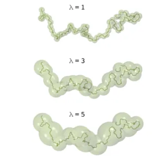
The initial configuration is first relaxed for 20 ns following a three-step procedure. After thermalization at a high temper-ature of 500 K in the constant-NVT ensemble for 10 ns, the system is cooled down with a linear temperature gradient of 100 K ns−1during 2 ns to reach the target temperature 300 K. The final equilibration step consists of an 8 ns run in the constant-NPT ensemble at 300 K and 0.1 MPa. The high-resolution atomistic reference trajectory; is then produced in the constant-NPT ensemble with independent control of the x, y, and z components of the external barostat stress tensor. We remind that the volumefluctuations are also taken into account as one of the degrees of freedom,16 thereby ensuring the correct pressure behavior of the optimized CG potentials. The trajectory is recorded every 50 fs, which is the desired DPD time stepΔt. In practice, only few hundred configurations are required, typically 500, as the Bayesian optimization method converges very fast as already mentioned in a previous paper.16 The coarse-graining procedure takes the same route as recent work by Lemarchand et al.15One, two, three, four, or five monomers are grouped together to build one mesoscopic bead as described inFigure 1. The degree of coarse-grainingλ

refers to the number of monomers per grain. For example, a degree of coarse graining ofλ = 3 means that each CG bead contains three monomers, that is, 12 UA. The position of the bead matches with the center of mass of the group of considered atoms all along the reference trajectory;. Another more sophisticated approach will be presented at the end of this paper. The velocity of the CG bead is computed from the difference between two consecutive positions separated by Δt. In the same way, the total force acting on a CG grain at each DPD time step is derived from its acceleration using Newton’s equation of motion. Furthermore, a bond between two UAs belonging to two different CG grains is kept in the CG model by adding one mesoscopic bond between the center of mass of the corresponding two CG beads.

Table 1. Important Basis Functions for Which an Analytic Optimization Can Be Performeda

model basis function Examples

power laws 1/rn _{Lennard-Jones}

polynomials rk _{harmonic bonds or angles}

tabulated Constant fitted to any potential

trigonometric cos kϕ Fourier dihedral potentials

a_{Note that the coefficients of the linear combination may not be the}

usual parameters of the standard forcefields, but the conversion is straightforward. For example, i

k jjj y_{zzz ϵ

( )

( )

Figure 1.Coarse-graining procedure of a cPB polymer chain. From top to bottom, a CG bead is built from 1, 3, or 5 monomers, corresponding to a degree of coarse-graining λ of 1, 3, or 5, respectively.

3. CHOICE OF THE FUNCTIONAL FORM FOR THE INTERACTIONS

Conservative nonbonded interactions were modeled by a pairwise potential depending only on the distance between grains. Grains are therefore considered spherical, although they may represent an elongated, flexible portion of a polymer chain. For this reason, the centers of mass of two grains may come close to each other. Lennard-Jones interactions would prevent such a behavior because of the divergence at r→ 0. In addition, it is desirable to allow for moreflexibility in the shape of the interaction potential by using more than two free parameters. A tabulated potential is an interesting alternative, for which we opted atfirst because it works well for pentane. Basis functions for the force were then chosen to be regularly spaced triangular functions, which amounts to a linear interpolation between tabulated points. The drawback of this functional form is that at r → 0, there is a considerable uncertainty on the force because such small distances are too rare in the reference trajectory (seeFigure 2a). The problem is

that the density is very sensitive to the errors on the force even at r → 0. Therefore, we decided to try smoother functions, namely, piecewise polynomials as was done by Das and Andersen.38 To be more specific, we split the distance range into two regions r≤ rmand rm≤ r ≤ rc, where the force is built

as a piecewise polynomial obtained from a combination of Bernstein polynomials.39The continuity and differentiability at the boundaries of each region are ensured by a linear combination of Bernstein basis functions as well. Using two

regions allows to choose independent enough function shapes for the attractive (shallow minimum) and repulsive parts, which is possible to adjust by adequately choosing the position of the intermediate cutoff rmand the degree of the polynomial

in each region.

The force exerted by bead j on i is thus expressed as l m ooooo o n ooooo o

∑

with xkthe weighting factor of the Bernstein basis polynomial

Pkas presented inFigure 3, r =|ri− rj|, eijthe unit vector in the

directionri− rj, and rcthe conservative cutoff.

The main advantages of using analytic Bernstein basis polynomials instead of tabulated potentials for the nonbonded pairwise interaction are given in the following:

• The extrapolation where no statistics exists, for instance, at r→ 0, is straightforward.

• It is easy to manage the continuity and differentiability of Bernstein functions.

• No mathematical artifact due to interpolation (linear, spline, bit-mapping, ...) or smoothening, especially because these kinds of soft CG potentials are highly sensitive to smallfluctuations.

• Few parameters (one per basis function) are required. Bonded interaction is a key feature for polymers, which was absent in the model for pentane. We chose to include bond as well as angle potential in order to allow for a bending stiffness. It seems overkilling to include also a dihedral potential, although a subtle dihedral structure can be observed in the reference trajectories at the smallest coarse-graining level. We opted for harmonic bond and angle potentials because no noticeable improvement was gained by using higher-order polynomials.

= −

E_bond( )r k r_b( r₀)2 (5)

θ = θ−θ

E_bend( ) k_a( ₀)2 (6)

By expanding the bonding and bending potentials, we get four additional conservative terms to optimize x6 = kb, x7= Figure 2.Optimized pairwise nonbonded conservative force (a) and

potential (b) for cPB at a degree of coarse graining ofλ = 5. The red circles refer to the optimized model using a linear combination of triangular basis functions, effectively corresponding to tabulated force and potential. The blue lines result from the linear combination of the weighted Bernstein basis polynomials plotted inFigure 3. Note that Guenza and co-workers have obtained a similar shape of the potential, with only a weak attractive part at the long range using the integral equation method for high coarse-graining levels.40,41

Figure 3.Typical set of Bernstein basis polynomials. rmdelimits the two regions used to define these functions. Their weighted sum corresponds to the optimized pairwise nonbonded conservative force to model cPB with a degree of coarse graining of 5 as drawn inFigure 2. The functional forms of the basis functions represented in this figure are given in theSupporting Information.

k_br₀, x₈= k_a, and x₉= k_aθ₀. Thus, we end with a typical set of conservative parameters to optimize xC= {x0, x1, ..., x9}.

With regard to the nonconservative interactions, we use the standard pairwise DPD form with the following dissipative interaction between beads i and j:

l m ooooo o n ooooo o i k jjjjj y_{zzzzz γ = − − · < ≥ → f v e e r r r r r r 1 for , 0 for j i ij ij ij D d 2 d d (7)

The parameterγ is optimized analytically and is the same for all pairs of grains including bond neighbors.vijis the relative

velocity v_i − v_j. r_d is the cutoff beyond which the nonconservative interaction vanishes andeijis the unit vector

from bead i to bead j.

In addition to the aforementioned parameters, several nonlinear parameters can be optimized.Figure 4 shows for a

degree of coarse graining ofλ = 1 how the likelihood of the reference trajectory changes with the intermediate cutoff r_m defined in Figure 3. It can be seen that the optimal value is close to 5.5 Å. On the other hand, test DPD runs were performed with the models optimized at all values of rm. The

density of the DPD runs in the NPT ensemble was calculated. Although all values are within a few percent of the MD target, the agreement is better for 6 < r_m < 8. Therefore, the parameters that give the highest probability to reproduce the reference trajectory may not be the parameters for which density is better reproduced. Our interpretation is that the Bayesian optimization tries to reproduce the full trajectory and has to compromise between all the potentially contradictory

observables. This leaves us with the option of choosing either the“best” value of the parameters or a suboptimal value but favoring a specific target property such as density. We suggest to take the latter option because we could not identify which other observable was harmed in this case. We recall that all the linear parameters are still optimized for the highest p(;|x).

The other nonlinear parameters were as follows:

• The conservative cutoff rc. The optimal value is beyond

50 Å forλ = 5. However, we decided not to increase rc

more than this value for computational efficiency. • The dissipative cutoff rd. The optimal value forλ = 1 is

about 9 Å, which also corresponds to the best reproduction of the diffusion coefficient of the monomers.

• The screening (or weighting) factors. They determine how much of the nonbonded interaction is applied between grains that already interact through bonded interactions either directly (1−2 bond) or through intermediate bonds (1−3 angle and 1−4 dihedral partners). The 1−2 bond weighting factor has only minor impact on the quality of the CG model whatever the degree of coarse graining chosen. Yet, forλ ≥ 2, the 1−3 angle and 1−4 dihedral weighting factors have a huge impact on thefinal behavior of the CG model. Low values allow better reproduction of the density but cause bad control of the structure of the polymer chains, which tend to fold back on themselves. With regard to these findings, the best choice for these two screening coefficients is 1 except for the lowest degree of coarse graining λ = 1 where the optimal 1−3 angle factor is strongly coupled with the choice of rmand was found to

be more suited at 0.5. These conclusions are also true according to the highest p(;|x).

• The DPD time step Δt.

4. CHOICE OF THE GRAIN DEFINITION

4.1. Impact of the Degree of Coarse Graining. 4.1.1. Main Results. Henderson42

demonstrated in 1974 that “two pair potentials which give rise to the same RDF cannot differ by more than a constant”. Yet, Potestio12illustrated the nonapplicability in practice of Henderson’s theorem. Indeed, because of numerical accuracy, there is no way to predict the response of a given system from the mere knowledge of its potential energy function. Consequently, the faithfulness of a CG model to the underlying high-resolution MD model has to be evaluated by running a simulation.

Therefore, every single newly optimized CG model was tested by running a 10 ns DPD simulation (5 ns equilibration and 5 ns production) in the constant-NPT ensemble starting from a well-equilibrated initial state obtained by coarse graining of a relaxed atomistic configuration. Even though the DPD simulations are much faster than MD (by a factor 20 atλ = 1 for r_d= r_c= 20 Å; by a factor 100 atλ = 5 for r_d= r_c= 40 Å), such a short DPD run is sufficient to evaluate the quality of the CG model because few nanoseconds are enough to see if the thermodynamic and structural properties are preserved or not (see Figure S1 in the Supporting Information). Of course, longer runs would be more precise but are not affordable considering the large number of tests (thousands). Several criteria were measured to check the validity of the model parameters. These results were compared to their respective targets obtained beforehand from the

Figure 4. λ = 1 (a) likelihood of the best set of unknown model parameters as a function of the delimiter rmbetween the Bernstein basis functions as described inFigure 3. Other nonlinear parameters were maintained constant rd= rc= 20 Å, and the screening factors for conservative interaction 1−2 bond, 1−3 angle, and 1−4 dihedral partners were set at 0, 0.5, and 1, respectively. The optimal value of rm corresponds to the minimum around 5.5 Å. (b) Equilibrium density obtained after running a DPD simulation. rm= 5.5 Å, although quite good (without hand-tuning), is not the optimal value for reproducing density.

analysis of CG MD (MDCG) trajectories for thefive degrees of coarse-grainingλ. The target functions were averaged over five 50 ns long statistically independent MDCG trajectories to account for slow decorrelation of the polymer chains at 300 K and ensure a convenient description of the phase space. Thermodynamic properties (density, pressure, and temper-ature) were followed over time. Local structure was also investigated by computing the following distribution functions: the nonbonded RDF g_nb(r) between two beads of different polymer chains or belonging to the same molecule but not directly connected together through a mesoscopic bond, the 1−2, 1−3, and 1−4 bonding distributions gbond(r) between two

beads connected through 1, 2, or 3 bonds in the polymer chain, and the bending distribution gbend(θ) between three

consec-utive beads. At the scale of the polymer chain, the evolution of the mean-square end-to-end distance⟨Ree2⟩, the mean-square

radius of gyration⟨R_g2_{⟩, and their ratio were also tracked over}

time as well as their distribution. From a dynamic point of view, we also studied the decorrelation of the end-to-end vector and the mean-square displacements (MSDs) of both the center of mass of a polymer chain and the CG grain.

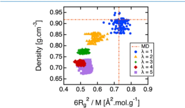
Figure 5 summarizes our work. The equilibrium DPD density is plotted versus 6⟨R_g2_{⟩/M. In other words, one}

thermodynamic property is plotted against one long-range structural characteristic. These two properties were chosen among others (diffusion coefficient, ...) because of their high importance to explicitly model cPB melts. One point on this map represents the result of the DPD run in the constant-NPT ensemble using one given optimized CG model. The MD target is represented by the intersection of the dashed lines. While the target density remains constant equal to 0.917 g cm−3 regardless of the degree of coarse graining, the target 6⟨Rg2⟩/M slightly changes with λ. Indeed, the coarse-graining

procedure of a polymer chain entails the loss of part of its tails. The typical loss is about the size of one mesoscopic bond between two consecutive CG beads given by the bonding distribution gbond(r), resulting in a target normalized

mean-square radius of gyration of 0.69(14) Å2_{mol g}−1_{atλ = 5, while}

the target value 0.72(15) Å2 mol g−1atλ = 1 is only faintly lower than the target 0.73(15) Å2 _{mol g}−1 _{before coarse}

graining.

Atλ = 1, the optimized CG model is always good because both the density and 6⟨R_g2_{⟩/M do not exceed 8% error with}

respect to MD, and this whatever the choice of the functional form for the interactions between the CG grains. When λ increases, the CG models become less and less accurate. To put it in another way, the higher theλ, the further the distance from the MD counterpart. Das and Andersen43and Dunn and Noid44,45have noticed the same tendency and proposed to add a volume potential independent of the grain configuration. This could surely improve the reproduction of density but is limited to homogeneous isotropic systems without interfaces. Another option would be to introduce many-body interactions based on the local density.30,46−48Forλ ≥ 2, the equilibrium density in the constant-NPT ensemble is underestimated although pressure optimization is included in the Bayesian optimization method, meaning that the CG potentials are not enough attractive (or too much repulsive) to maintain the volume. This deviation is higher with λ reaching about 20% underestimation forλ = 5. On the other hand, we verified that the ratio of⟨Ree2⟩ over ⟨Rg2⟩ approximately equals 6 whatever

the degree of coarse graining or the CG model chosen, meaning that the polymer chains follow the expected Gaussian behavior.49 However, their packing differs depending on the degree of coarse graining chosen. For λ ≥ 3, 6⟨Rg2⟩/M =

0.52(6) Å2 mol g−1, traducing collapsing of the polymer molecules. Interestingly, both the density and the packing of the polymer chains do not change that much with the CG model at givenλ. This result indicates that the initial choice of the nonlinear parameters we played with, that is, the conservative cutoff rc, the dissipative cutoff rd, and the

functional form of the Bernstein polynomials, does not impact as much as thefinal result. The Bayesian method adapts the linear parameters in consequence. For instance, a shorter conservative cutoff r_cimplies a shift of the attractive part of the nonbonded CG potential to smaller distance.

We note here, and this is a recurring feature in the following, that the CG model is better at small coarsening levels. This is unexpected because the Markovian approximation of our DPD model and the assumption of pairwise additive stochastic forces50 are better found14 at higher degree of coarsening, where the separation of time scales should be more marked.

4.1.2. Thermodynamic Properties. From now, we only consider the “best” CG model for each λ according to the distance from target MD as described inFigure 5. Each CG model was taken to run 110 ns DPD simulations (10 ns equilibration and 100 ns production) in the constant-NPT ensemble. In the same spirit, an additional 110 ns DPD run in the constant-NVT ensemble at the target density 0.917 g cm−3 was carried out. Both the equilibrium density and pressure are presented inTable 2. Unsurprisingly, atλ = 1, there is no huge difference between the NVT and the NPT simulations, reflecting the equivalence of statistical ensembles. At λ = 2, the average pressure necessary to maintain the correct volume is about 100 times higher than the target 0.1 MPa. As λ increases, this average pressure decreases again, reaching only 30 times the target for λ = 5. Therefore, for large λ, even though the NPT DPD density is farther below the MD target, the average pressure necessary for recovering the correct density is smaller because the model is more compressible. Indeed, as expected, the larger the degree of coarse graining, the softer the potential and the higher the sensitivity of the CG model to pressure.

Figure 5. Equilibrium density vs six times the normalized mean-square radius of gyration measured over 5 ns of a DPD simulation as a function of the degree of coarse-grainingλ. Each point on this map corresponds to the trial of one optimized CG potential for various rm (between 3 and 15 Å) and rc(between 18 and 50 Å). The screening factors for conservative interaction between 1−3 angle and 1−4 dihedral partners were set to 1 forλ ≥ 2.

4.1.3. Structural Properties. The nonbonded RDF gnb(r)

(RDF) obtained in DPD in the NVT and NPT ensembles is compared with their respective MDCG targets inFigure 6. At

λ = 1, the agreement between the three RDFs is outstanding, even though the optimization protocol is not based on it in contrast with other methods as already mentioned in the Introduction. Atλ = 2, the RDFs produced in the NVT and NPT ensembles are almost perfectly matching, although the equilibrium density in the NPT ensemble is 7% lower than the MD reference (Table 2). This demonstrates again that exclusively looking at the RDF is not sufficient to get a good CG model, especially if considering the pressure behavior. For higher degree of coarse graining, the difference between the two RDFs obtained in DPD becomes more visible. The RDF

produced in the NPT ensemble is shifted to larger distances than the one produced in the NVT ensemble in accordance with the thermodynamic measurements. Moreover, these two RDFs are systematically shifted to further distances with respect to the MDCG target. At λ = 5, the RDF at short distance is above the MDCG reference, meaning that the soft CG beads are interpenetrating each other much more than they should. This behavior is balanced by a repulsive slope more gentle than in the MDCG reference.

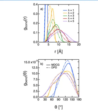
The intramolecular structure of the polymer chain has also been investigated as a function of the degree of coarse graining. The bonding distributions gbond(r) between two consecutive

beads are given inFigure 7a. We also report inFigure 7b the

bending distribution g_bend(θ) between three consecutive beads forλ = 1, λ = 2, and λ = 5. As before, the agreement between DPD and MD is excellent for the smallest degree of coarse graining. Forλ ≤ 3, both the reference bonding and bending distributions exhibit two highly superimposed peaks that disappear when increasing λ, whereas the distributions produced with DPD only present one peak shifted to smaller distances/angles. The local structure of the polymer chain is thus too much packed. Replacing the harmonic bonds/angles by quadratic or cosine-based potentials did not really improve our observations.

We now focus on the long-range structural properties of the polymer chains.Figure 8shows the computed distribution of the end-to-end vector in DPD using the“best” CG models for λ = 1, λ = 2, and λ = 5. The distribution of the end-to-end vector obtained atλ = 1 matches very well with MD. By the way, the target distribution function is slightly different depending on the degree of coarse graining because of the loss of the tails of the CG polymer chain as discussed before. For clarity, only the MD end-to-end vector distribution is Table 2. Equilibrium Density and Pressure Measured over

100 ns of DPD Simulation Performed in the Constant-NVT and Constant-NPT Ensembles Using the “Best” CG Potential for Each Degree of Coarse-Grainingλa

NVT (T = 300 K) NPT (P = 0.1 MPa, T = 300 K) Pmeasured[MPa] ρ [g cm−3] Pmeasured[MPa] ρ [g cm−3]

λ = 1 0.24± 0.077 0.917 0.09± 0.10 0.917

λ = 2 9.7± 1.7 0.917 0.14± 0.09 0.852

λ = 3 7.4± 2.6 0.917 0.07± 0.03 0.780

λ = 4 5.5± 1.5 0.917 0.12± 0.60 0.724

λ = 5 2.9± 1.0 0.917 0.12± 0.13 0.726

a_{The target density is 0.917 g cm}−3_{at 300 K and 0.1 MPa.}

Figure 6.Nonbonded RDFs produced in the constant-NVT and the constant-NPT ensembles at T = 300 K and P = 0.1 MPa using the “best” CG model for various degrees of coarse graining, respectively. (a)λ = 1. For a better view, a small vertical offset of 0.05 is added to the RDF produced in the NVT ensemble. (b)λ = 2. (c) λ = 3. (d) λ = 4. (e)λ = 5.

Figure 7.Bonding (a) and bending (b) distributions as a function of the degree of coarse-grainingλ. The full and dotted lines represent the MDCG and DPD results, respectively. The two bonding distributions atλ = 1 were trimmed for greater clarity. For the same reason, the bending distributions obtained for λ = 3 and λ = 4 are not represented.

plotted. When increasingλ, we notice a shift of the end-to-end vector to smaller distance. This effect is a direct repercussion at long distance of the local packing of the bonds and angles of the polymer chain (seeFigure 7).

In a polymer melt, Flory’s theorem states that the polymer chains are nearly ideal.51In this case, it can be shown49that the probability distribution function of the end-to-end distance p(R_ee) is a Gaussian distribution given by

i k jjjjj π y_{zzzzz i_kjjjjj y_{zzzzz π = ⟨ ⟩ − ⟨ ⟩ p R R R R R ( ) 3 2 exp 3 2 4 ee ee 2 3/2 ee2 ee 2 ee 2 (8)

Figure 8 confirms the validity of this law for absolutely all our models. Another confirmation comes from the ratio ⟨Ree2⟩/⟨Rg2⟩ that equals 6 in all cases as detailed inTable 3.

While the structural properties of our different CG models do not reproduce exactly the MD, especially for large λ, the polymer chains are still Gaussians as expected when considering a polymer melt.

4.1.4. Dynamics. In this section, we present some dynamical properties. Thefive “best” CG potentials were taken again to run 1μs long simulations in the NVT ensemble at the target densityρ = 0.917 g cm−3in order to avoid any undesired box size effects as for instance faster dynamics because of low density.

The end-to-end vector autocorrelation function has been computed in MD and using the different CG models. Results are plotted in Figure 9a. In the reference MD trajectory, the end-to-end vector completely loses its initial orientation after a few hundred of nanoseconds, whereas this time is reduced to about 10 ns for λ = 5. For completeness, the characteristic relaxation timeτ of the polymer chains has been computed for eachλ by integrating the fit of these autocorrelation functions using the Kohlrausch−Williams−Watts stretched exponential form.52 i k jjjjj i_kjjj y_{zzz y { zzzzz i_kjjjj y_{zzzz

∫

In MD,τ equals 107 ns, whereas its value is only around 2 ns for the highest degree of coarse graining (Table 4). As it is often seen in DPD simulations,53 the higher the degree of coarse graining, the faster the decorrelation of the end-to-end vector.

The MSD of the center of mass of the polymer chains is presented in Figure 9b. The self-diffusion coefficient of the polymer chains + can be derived from the MSD using the classical formula = ⟨ − ⟩ →+∞ + t r t r 1 6 lim d d ( ( ) (0)) t 2 (10)

As we can see inFigure 9b andTable 4, we found that the diffusion of the polymer chains becomes faster when increasing

Figure 8.Distributions of the end-to-end distance in MD (black) and for various degrees of coarse graining (colors). The dotted lines correspond to the direct application ofeq 8using the measured⟨Ree2⟩ for each MD and DPD simulation.

Table 3. Average Structural Properties of cPB in MD and DPD Using the“Best” CG Potential at Each λ

⟨Ree⟩ [Å] ⟨Rg⟩ [Å] ⟨Ree2⟩/⟨Rg2⟩ MD 45.9± 0.9 19.3± 0.2 6.2± 0.1 λ = 1 45.4± 0.9 19.7± 0.1 5.9± 0.2 λ = 2 40.1± 0.7 17.2± 0.2 6.0± 0.1 λ = 3 38.2± 0.5 16.4± 0.1 6.0± 0.1 λ = 4 36.7± 0.4 15.9± 0.1 5.9± 0.1 λ = 5 37.9± 0.5 16.5± 0.1 5.8± 0.1

Figure 9.(a) Decorrelation of the end-to-end vector in MD (black dots) and DPD (dotted colors). The full lines correspond to thefit using Kohlrausch−Williams−Watts stretched exponentials. (b) MSD of the center of mass of the polymer chain in MD (black) and DPD (colors). The dashed and dotted lines represent slopes of 2 (ballistic regime) and 1 (diffusion regime), respectively.

Table 4. Relaxation Timeτ of the End-to-End Vector and Diffusion Coefficient +of the Center of Mass of the Polymer Chain Computed UsingEqs 9and10a

τ [ns] + [10−12m2_s−1_] MD 107 9.9± 0.3 λ = 1 39 18± 1 λ = 2 10 63± 4 λ = 3 4 141± 12 λ = 4 3 185± 6 λ = 5 2 244± 9

a_{Both values were measured in the constant-NVT ensemble in MD}

λ. This is contrary to the recent work of Lemarchand et al.15 using the FM method. Yet, in contrast to their work, the dynamics at short time in the ballistic regime (scaling as t2_{) is}

apparently well reproduced. We will discuss this in detail in the following section. Moreover, Dequidt and Canchaya16already showed the strong dependence of+with the initial choice of the dissipative cutoff rd. Because of the numerous amount of

nonlinear parameters, we decided to keep rd= rcin most of our

trials. We only performed one iterative optimization of rdforλ

= 1 withfixed other nonlinear parameters, that is, quadratic bonds, harmonic angles, rm= 7 Å, rc= 20 Å. In this case, the

optimal dissipative cutoff rd was found to be more suited at

around 9 Å instead of 20 Å, both according toln (p ;|x)and in terms of monomer subdiffusive motion.49

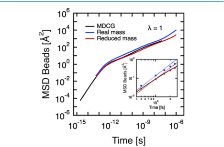
4.2. Choice of the DPD Time Step.Figure 10 displays the MSD of the CG grains forλ = 1 obtained in DPD using a

time step ofΔt = 50 fs. At t = 50 fs, that is, the first DPD step, we notice that the local dynamics of the bead is already too fast with respect to the reference MDCG MSD. Let us first underline that in our simulations, temperature and velocity obey the theorem of equipartition of energy expressed as

= ⟨ ⟩ RT M v 3 2 1 2 2 (11)

where R is the universal gas constant, T is the temperature, M is the molar mass of the CG bead, and⟨v2⟩ is the mean-square velocity of the group of beads. Additionally, with the help of the velocity-Verlet algorithm, it is easy to prove that the MSD at twice the simulation time step 2Δt can be predicted before running any simulation whatever the thermostat, that is,

⟨( (2r Δt)−r(0))2⟩ =(2Δt)2⟨ ⟩v2 (12)

This equation is verified in the inset ofFigure 10because the MSD obtained in DPD crosses perfectly at t = 2Δt with the theoretical ballistic straight line MSD = 3RT/Mt2. Because of both the integration algorithm and the theorem of equipartition of energy, we propose the use of an effective

molar mass in order to be able to reproduce the dynamics of the bead at short time scales, in particular, at 2Δt. By combiningeqs 11and12, we obtain the effective molar mass of the grain = Δ ⟨ Δ − ⟩ M RT t r t r 3 (2 ) ( (2 ) (0)) effective 2 2 (13)

A summary of the required mass correction for various choices ofΔt and λ is given inTable 5. ForΔt = 50 fs, the

mass of the bead needs to be enhanced by 52% for λ = 1, whereas only 12% increase is required forλ = 5. The larger the degree of coarse graining, the higher the DPD time step is allowed before mass adjustment becomes critical.

Once the mass correction is done, the linear parameters are optimized accordingly using the Bayesian method. Using this new CG model, we observe a better agreement at short time between DPD and the reference MDCG MSD as shown in Figure 10. This result also confirms the good setting of γ, as supplied by the Bayesian method. The matching of the mass-corrected model with its MDCG counterpart is also improved at long time scales. Forλ = 2, the mass correction (seeTable 5) l e a d s t o l o w e r i n g o f t h e d y n a m i c s w i t h

= ± × − −

+ 33 3 10 12m s2 1with mass adjustment instead of

= ± × − −

+ 63 4 10 12m s2 1 without. We could have im-proved these results even more by optimizing again the full set of nonlinear parameters, in particular, the dissipative cutoff r_d, taking into account the mass correction.

To go further, the DPD time step Δt can be optimized as well. Note that the CG models should be used at the time step for which they were optimized. A priori, using them with a different time step will yield different results unless time steps are below 10−20 fs.54 However, using longer time steps is more interesting to reach the relevant time scales for which CG models are developed.Figure 11shows how the choice ofΔt affects the MSD of the CG grains for the highest degree of coarse-grainingλ = 5. At this level, large time steps are allowed, thanks to the softness of the corresponding CG potentials. Figure S2 displays the corresponding optimized pairwise nonbonded conservative potentials. Interestingly, the dynamics is improved as Δt increases. For Δt = 1 ps, the diffusion coefficient + of the center of mass of the polymer chain is slowed down to 40.1± 1.1 × 10−12m2s−1, which is still faintly too high with respect to MD, but is much better than forΔt = 50 fs without mass correction (seeTable 4). We verified that the thermodynamic properties and the structural properties remain roughly unchanged whatever the choice of Δt (see Figure S3 in the Supporting Information). In particular, the equilibrium density obtained from a DPD simulation in the

Figure 10.MSD of the CG beads at λ = 1 obtained from the CG reference trajectory MDCG (black) and from DPD (blue and red) with a DPD time step Δt = 50 fs. In the inset, the dotted lines represent the theoretical ballistic regime MSD= 3RT_Mt2 with R the universal gas constant, T = 300 K, and M the molar mass (with/ without mass correction) of one CG bead. The full circles effectively correspond to the MSD obtained in DPD. In blue, the real CG bead mass M = 54.090 g mol−1is used. In red, the mass of the grain is corrected according toeq 13, resulting in M = 82.235 g mol−1as given inTable 5.

Table 5. Required Mass Correction as a Function of the Degree of Coarse-Grainingλ and the Desired DPD Time StepΔt

Δt [fs] 50 100 200 500 1000

molar mass

[g mol−1] effective molar mass [g mol−1]

λ = 1 54.09 82.2 108.1 178.2 483.7 1263.4

λ = 2 108.2 135.1 165.5 251.6 627.2 1587.5

λ = 3 162.3 189.9 226.4 330.5 778.9 1925.4

λ = 4 216.4 248.2 292.1 418.2 951.6 2265.0

constant-NPT ensemble is systematically around 0.72± 0.02 g cm−3 as observed before for λ = 5 (Figure 5). Nevertheless, without mass adjustment, both the dynamical and the structural properties deteriorate asΔt increases.

4.3. Shape of the CG Beads. In order to understand why the CG model is better at the small coarsening level, we investigated the conformations adopted by the CG beads at the different levels of coarse graining from 1 to 5 monomers per bead. Should the shape and the orientation of the grains be used as additional degrees of freedom in the CG model?29The high-resolution MD trajectory ; was taken to compute the gyration tensorR_gbead_{of each bead defined such as}

∑

∑

where N is the number of UA inside the considered grain, w_i= mi/∑j=1N mjis the weight fraction of atom i in the grain,riis the

position of the atom i, andr_g is the position of the center of mass of the considered grain. The gyration tensor describes the shape adopted by the grain at the lowest relevant order. By construction, this tensor is a real symmetric matrix. Such a matrix possesses three positive eigenvaluesλ₁,λ₂,λ₃and their corresponding three eigenvectors v1, v2, v3 form an

orthonormal basis. The eigenvector corresponding to the largest eigenvalue represents the principal axis of the bead. As introduced by previous authors,55,56 we compute the asphericity ( given by the formula

λ λ λ = ∑ − ∑ λ≥λ = ( ( ) 2( ) i j i i 2 1 3 2 i j (16)

This quantity ranges from 0 to 1. The asphericity of a spherical conformation is zero, while it reaches 1 for a stick. The distribution of the asphericity averaged over all CG beads across the trajectory is drawn for eachλ inFigure 12. Whatever the degree of coarse graining, the shape of the distribution is the same if considering one random CG grain in the middle of a polymer chain or one at the tail. This confirms that all beads follow the same evolution rule. At low degree of coarse

grainingλ = 1, that is, one monomer per bead, the distribution of the asphericity exhibits a sharp peak at 0.52, traducing a well-defined structure. In fact, from a geometrical point of view, the repeating unit of the cPB looks like a thin cuboid because of the rigid carbon−carbon double bond in its middle. In addition, still for λ = 1, the distribution width is directly related to the small bond and angle fluctuations at the atomistic level. At λ = 2, the distribution of ( is mainly divided into two strongly overlapped peaks centered at 0.52 and 0.73. A slight bump at 0.3 also appears. Two consecutive repeating units of the cPB are connected by aflexible sigma bond. Thus, the resulting CG bead becomesflexible as well. At higher degree of coarse graining, the distribution of the asphericity gets broader ranging from 0.2 to 0.9. Indeed, the CG bead holdsλ − 1 sigma bonds connecting the repeating units together, leading to more and moreflexibility.

We now focus on the dynamical behavior of the shape of the CG beads over time in the reference trajectory. First, we consider the square root of the three positive eigenvaluesλ1,λ2,

andλ₃denoted as a, b, and c, respectively. We report inFigure 13a the time evolution of these three characteristic lengths for

Figure 11.MSD of the CG beads at λ = 5 obtained from the CG reference trajectory MDCG (black) and from DPD (colors) for various DPD time stepsΔt. Mass adjustment is included as given in

Table 5.

Figure 12.Distribution of the asphericity as a function of the degree of coarse graining. The cPB repeating unit is drawn for comparison.

Figure 13.Shape (a) and orientation (b) of one bead at a degree of coarse graining of λ = 5, that is, containing five repeating units as drawn inFigure 12. (a) Time evolution of the three characteristic lengths a, b, c. (b) Time evolution of the three coupled deviation anglesθ = arccos(v(t + Δt)·v(t)) of the eigenvectors with themselves.

one CG bead atλ = 5. At t = 0 ps, the bead is elongated along one principal direction as a≫ b,c. Then, the principal length a steadily decreases for the benefit of b. From t = 110 ps to t = 280 ps, the shape of the grain remains stable. An abrupt change occurs at t = 280 ps with a typical characteristic time of 1 ps. This kind of scarce event correlates well with the unfolding of a dihedral angle at the atomistic level. Therefore, a CG model that aims to take into account both the shape of the bead and its time evolution will have to include these short and long time scale phenomena.

Second, we consider the orientation of the bead over time. We compute the deviation angle of an eigenvector with itself after one DPD time step, that is, betweenv₁(t) andv₁(t +Δt) (the same relation can be written for the other two directions). Figure 13b displays the evolution of the three deviation angles. By construction, they form an orthonormal basis. The rotation of one vector implies the rotation of another vector by the same amount, leading to two-by-two symmetrical results. Strikingly, the deviation angle reaches sometimes very high values up to 90°. These events occur when two characteristic lengths are nearby as we can see inFigure 13a, leading to the loss of two principal orientations. Reproducing such a trajectory including bead orientation is a challenge because of these rotational “jumps” of the principal axes. The other option is to use not only the orientation but the whole gyration tensor as a degree of freedom of the CG model, with specific evolution equations (to be specified) describing the dynamics of the grain shape.

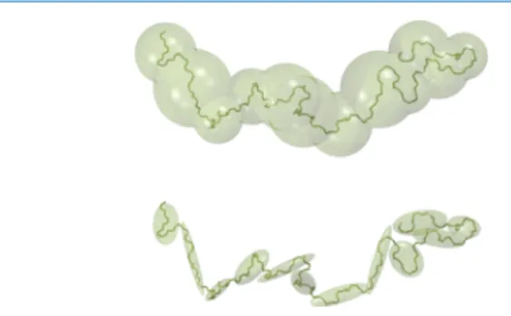
The shape of the CG bead is an intrinsic characteristic of the chemical microstructure. In classical CG models as we used in this study, one bead is only represented by its center of mass and the beads interact with each other through pairwise interactions. Consequently, all the information about the shape of the CG grain is lost. In practice, thefine analysis of the high-resolution reference trajectory; shows that the CG grains are almost never spherical (( does not reach 0 inFigure 12), as they represent flexible portions of a linear polymer chain. Considering this, a second-order approximation is used to model the CG grain as aflexible ellipsoid.Figure 14gives an idea of the difference between these two visions for λ = 5. 5. CONCLUSIONS AND PERSPECTIVES

In this paper, we have successfully applied the recent Bayesian optimization approach to cPB polymer melts. Effective CG models are derived from the analysis of CG atomistic reference

trajectories ;. The conservative interactions were modeled using analytical forms, namely, harmonic potentials for the bonding and bending terms and piecewise polynomials for the nonbonded terms. The dissipative interactions were modeled using the standard pairwise dissipative force where the friction parameterγ was obtained using the Bayesian method.

The faithfulness of the CG models to the higher resolution model has been quantified for various choices of the functional form for the interactions between CG beads. The choice of the intermediate rm and conservative rc cutoffs does not impact

that much the thermodynamic and the structural properties of the polymer chains for a given coarse-graining level, as the Bayesian method adapts the linear parameters accordingly. For λ ≥ 2, a strong coupling was found between the setting of the intramolecular nonbonded screening factors and the ability of the CG model to conveniently reproduce either the density or the structure of the polymer chain.

Our CG models are able to reproduce reasonably well the thermodynamic, the structural, and the dynamic properties of cPB melts. The polymer chains were found to follow Gaussian behavior as predicted by the theory for polymer melts. Atλ = 1, the agreement between MD and DPD simulations is excellent for all properties of interest. Nevertheless, as the degree of coarse-grainingλ increases, the properties obtained by running a DPD simulation using our CG models deviate more and more from their MDCG counterparts. The reason for this still needs to be elucidated. For example, atλ ≥ 2, the local structure is too packed with respect to MDCG, leading to a slight collapse of the polymer chains. From a dynamic point of view, the decorrelation of the end-to-end vector and the diffusion of the polymer chain become faster than MD as λ increases. We introduced the concept of effective mass to properly reproduce the dynamics at short times by keeping classical molecular simulation considerations (equipartition of energy, velocity-Verlet algorithm). This mass adjustment becomes crucial if one wants to use large DPD time steps. As far as we know, this has never been highlighted. At long time scales, the diffusion of the beads depends on the choice of the dissipative cutoff r_dand the DPD time stepΔt.

The higher the degree of coarse graining, the higher the compressibility of the resulting CG models, which results in lowering the equilibrium density, although the pressure has been taken into account in the optimization process. This effect is attributed to the choice of the grain definition. As already mentioned in previous work, the Bayesian optimization provides the“best” parameters of a given CG model in order to reproduce the full trajectory and not especially one individual observable among others. If the degrees of freedom (coarse-graining level, isotropy), the CG functional form (conservative and dissipative interactions), and the DPD time step are not well chosen, then the resulting CG force field will be poor. Especially, if a key physical feature is missing in the CG model, thefinal CG force field will never be appropriate. The radial pairwise approximation assumes that the interaction between CG beads depends only on their distance from each other, thus assuming that the beads are spherical. However, as the degree of coarse graining increases, the beads become more and more flexible and adopt a broad range of conformations. We also pointed out a strong anisotropy of the shape of the bead over long time ranges with respect to typical DPD time steps.

Atλ = 1, the radial pairwise approximation is sufficient as we were able to obtain outstanding CG potentials. This result is attributed to the following reason. At this level, the CG bead,

Figure 14.Two visions of coarse graining of a polymer chain at a degree of coarse-grainingλ = 5. At the top, one bead is represented by a sphere with twice (for better view) its radius of gyration as the radius; at the bottom, one bead is represented by an ellipsoid with twice (for better view) the square root of the eigenvalues of its tensor of gyration as the three characteristic lengths.

which corresponds to the repeating unit of the polymer, is rigid. We will provide in a forthcoming paper a detailed description of a refined realistic CG model for cPB at λ = 1 obtained by taking this bottom-up route based on trajectory matching. In particular, the transferability in temperature, pressure, and in terms of chain length will be addressed. In the future, we expect to be able to better model this system at large coarse-graining levels by considering the CG beads asflexible ellipsoids interacting with each other through anisotropic potentials. In this case, we believe in a better reproduction of the compressibility for the highest coarse-graining levels.

■

*

The Supporting Information is available free of charge on the ACS Publications website at DOI: 10.1021/acsome-ga.9b00144.

Atomistic forcefield parameters for cPB; time evolution of the density and the ratio 6⟨Rg2⟩/M during a 10 ns

DPD simulation using the“best” CG model for various degrees of coarse-graining λ; optimized pairwise non-bonded conservative potentials for cPB at a degree of coarse-graining ofλ = 5 for various choices of DPD time step Δt; and nonbonded RDFs produced in the constant-NPT ensembles at T = 300 K and P = 0.1 MPa using the mass-adjusted CG models developed at Δt = 5 for various DPD time steps Δt (PDF)

Time evolution of the bead size (AVI)

■

Corresponding Authors

*E-mail:Alain.Dequidt@uca.fr(A.D.). *E-mail:Patrice.Malfreyt@uca.fr(P.M.). ORCID

Alain Dequidt: 0000-0003-1206-1911

Patrice Malfreyt:0000-0002-3710-5418

Notes

The authors declare no competingfinancial interest.

■

This work was partially funded by the Investissements d’Avenir program”Développement de l’Economie Numérique” through SMICE project.

■

(1) de Gennes, P.-G. Scaling Concepts in Polymer Physics, 1st ed.; Cornell University Press, 1979.

(2) Gerroff, I.; Milchev, A.; Binder, K.; Paul, W. A new off-lattice Monte Carlo model for polymers: A comparison of static and dynamic properties with the bond-fluctuation model and application to random media. J. Chem. Phys. 1993, 98, 6526−6539.

(3) Harmandaris, V. A.; Kremer, K. Predicting polymer dynamics at multiple length and time scales. Soft Matter 2009, 5, 3920.

(4) Noid, W. G. Perspective: Coarse-grained models for biomolecular systems. J. Chem. Phys. 2013, 139, 090901.

(5) Müller-Plathe, F. Coarse-Graining in Polymer Simulation: From the Atomistic to the Mesoscopic Scale and Back. ChemPhysChem 2002, 3, 754−769.

(6) Reith, D.; Pütz, M.; Müller-Plathe, F. Deriving effective mesoscale potentials from atomistic simulations. J. Comput. Chem. 2003, 24, 1624−1636.

(7) Ercolessi, F.; Adams, J. B. Interatomic potentials from first-principles calculations: the force-matching method. Europhys. Lett. 1994, 26, 583−588.

(8) Izvekov, S.; Parrinello, M.; Burnham, C. J.; Voth, G. A. Effective force fields for condensed phase systems from ab initio molecular dynamics simulation: A new method for force-matching. J. Chem. Phys. 2004, 120, 10896.

(9) Li, Z.; Bian, X.; Yang, X.; Karniadakis, G. E. A comparative study of coarse-graining methods for polymeric fluids: Mori-Zwanzig vs. iterative Boltzmann inversion vs. stochastic parametric optimization. J. Chem. Phys. 2016, 145, 044102.

(10) Bayramoglu, B.; Faller, R. Modeling of polystyrene under confinement: exploring the limits of iterative boltzmann inversion. Macromolecules 2013, 46, 7957−7976.

(11) Maurel, G.; Goujon, F.; Schnell, B.; Malfreyt, P. Multiscale Modeling of the Polymer-Silica Surface Interaction: From Atomistic to Mesoscopic Simulations. J. Phys. Chem. C 2015, 119, 4817−4826. (12) Potestio, R. Is Henderson’s theorem practically useful? JUnQ 2013, 3, 13−15.

(13) Maurel, G.; Goujon, F.; Schnell, B.; Malfreyt, P. Prediction of structural and thermomechanical properties of polymers from multiscale simulations. RSC Adv. 2015, 5, 14065−14073.

(14) Hijón, C.; Español, P.; Vanden-Eijnden, E.; Delgado-Buscalioni, R. Mori-Zwanzig formalism as a practical computational tool. Faraday Discuss. 2010, 144, 301−322.

(15) Lemarchand, C. A.; Couty, M.; Rousseau, B. Coarse-grained simulations of cis- and trans-polybutadiene: A bottom-up approach. J. Chem. Phys. 2017, 146, 074904.

(16) Dequidt, A.; Canchaya, J. G. S. Bayesian parametrization of coarse-grain dissipative dynamics models. J. Chem. Phys. 2015, 143, 084122.

(17) Canchaya, J. G. S.; Dequidt, A.; Goujon, F.; Malfreyt, P. Development of DPD coarse-grained models: From bulk to interfacial properties. J. Chem. Phys. 2016, 145, 054107.

(18) Goujon, F.; Malfreyt, P.; Tildesley, D. J. Interactions between polymer brushes and a polymer solution: mesoscale modelling of the structural and frictional properties. Soft Matter 2010, 6, 3472−3481. (19) Español, P.; Zúñiga, I. Obtaining fully dynamic coarse-grained models from MD. Phys. Chem. Chem. Phys. 2011, 13, 10538.

(20) Ghoufi, A.; Malfreyt, P. Recent advances in many body dissipative particles dynamics simulations of liquid-vapor interfaces. Eur. Phys. J. E 2013, 36, 10.

(21) Harmandaris, V.; Kalligiannaki, E.; Katsoulakis, M.; Plecháč, P. Path-space variational inference for non-equilibrium coarse-grained systems. J. Comput. Phys. 2016, 314, 355−383.

(22) Izvekov, S.; Voth, G. A. A multiscale coarse-graining method for biomolecular systems. J. Phys. Chem. B 2005, 109, 2469−2473.

(23) Chaimovich, A.; Shell, M. S. Coarse-graining errors and numerical optimization using a relative entropy framework. J. Chem. Phys. 2011, 134, 094112.

(24) Rudzinski, J. F.; Noid, W. G. Coarse-graining entropy, forces, and structures. J. Chem. Phys. 2011, 135, 214101.

(25) Noid, W. G.; Chu, J.-W.; Ayton, G. S.; Krishna, V.; Izvekov, S.; Voth, G. A.; Das, A.; Andersen, H. C. The multiscale coarse-graining method. I. A rigorous bridge between atomistic and coarse-grained models. J. Chem. Phys. 2008, 128, 244114.

(26) Dunn, N. J. H.; Foley, T. T.; Noid, W. G. Van der Waals perspective on coarse-graining: progress toward solving represent-ability and transferrepresent-ability problems. Acc. Chem. Res. 2016, 49, 2832− 2840.

(27) Shell, M. S. In Advances in Chemical Physics; Rice, S. A., Dinner, A. R., Eds.; John Wiley & Sons, Inc.: Hoboken, NJ, USA, 2016; pp 395−441.

(28) Shell, M. S. The relative entropy is fundamental to multiscale and inverse thermodynamic problems. J. Chem. Phys. 2008, 129, 144108.

(29) Chaimovich, A.; Shell, M. S. Anomalous waterlike behavior in spherically-symmetric water models optimized with the relative entropy. Phys. Chem. Chem. Phys. 2009, 11, 1901.

(30) Sanyal, T.; Shell, M. S. Coarse-grained models using local-density potentials optimized with the relative entropy: Application to implicit solvation. J. Chem. Phys. 2016, 145, 034109.

(31) Poli, R.; Kennedy, J.; Blackwell, T. Particle swarm optimization. Swarm Intell. 2007, 1, 33−57.

(32) Plimpton, S. Fast parallel algorithms for short-range molecular dynamics. J. Comput. Phys. 1995, 117, 1−19.

(33) Smith, G. D.; Paul, W. United atom force field for molecular dynamics simulations of 1,4-polybutadiene based on quantum chemistry calculations on model molecules. J. Phys. Chem. A 1998, 102, 1200−1208.

(34) Tsolou, G.; Mavrantzas, V. G.; Theodorou, D. N. Detailed Atomistic Molecular Dynamics Simulation of cis -1,4-Poly(butadiene). Macromolecules 2005, 38, 1478−1492.

(35) Berendsen, H. J. C.; Postma, J. P. M.; van Gunsteren, W. F.; DiNola, A.; Haak, J. R. Molecular dynamics with coupling to an external bath. J. Chem. Phys. 1984, 81, 3684.

(36) Schneider, T.; Stoll, E. Molecular-dynamics study of a three-dimensional one-component model for distortive phase transitions. Phys. Rev. B 1978, 17, 1302−1322.

(37) Dünweg, B.; Paul, W. Brownian dynamics simulations without Gaussian random numbers. Int. J. Mod. Phys. C 1991, 02, 817−827.

(38) Das, A.; Andersen, H. C. The multiscale coarse-graining method. III. A test of pairwise additivity of the coarse-grained potential and of new basis functions for the variational calculation. J. Chem. Phys. 2009, 131, 034102.

(39) Natanson, I. P. Constructive Function Theory I: Uniform Approximation; Ungar Pub Co, 1964; Vol. I.

(40) Clark, A. J.; Guenza, M. G. Mapping of polymer melts onto liquids of soft-colloidal chains. J. Chem. Phys. 2010, 132, 044902.

(41) Dinpajooh, M.; Guenza, M. G. Coarse-graining simulation approaches for polymer melts: the effect of potential range on computational efficiency. Soft Matter 2018, 14, 7126−7144.

(42) Henderson, R. L. A uniqueness theorem for fluid pair correlation functions. Phys. Lett. A 1974, 49, 197−198.

(43) Das, A.; Andersen, H. C. The multiscale coarse-graining method. V. Isothermal-isobaric ensemble. J. Chem. Phys. 2010, 132, 164106.

(44) Dunn, N. J. H.; Noid, W. G. Bottom-up coarse-grained models that accurately describe the structure, pressure, and compressibility of molecular liquids. J. Chem. Phys. 2015, 143, 243148.

(45) Dunn, N. J. H.; Noid, W. G. Bottom-up coarse-grained models with predictive accuracy and transferability for both structural and thermodynamic properties of heptane-toluene mixtures. J. Chem. Phys. 2016, 144, 204124.

(46) Sanyal, T.; Shell, M. S. Transferable Coarse-Grained Models of Liquid-Liquid Equilibrium Using Local Density Potentials Optimized with the Relative Entropy. J. Phys. Chem. B 2018, 122, 5678−5693.

(47) DeLyser, M. R.; Noid, W. G. Extending pressure-matching to inhomogeneous systems via local-density potentials. J. Chem. Phys. 2017, 147, 134111.

(48) Wagner, J. W.; Dannenhoffer-Lafage, T.; Jin, J.; Voth, G. A. Extending the range and physical accuracy of coarse-grained models: Order parameter dependent interactions. J. Chem. Phys. 2017, 147, 044113.

(49) Rubinstein, M.; Colby, R. H. Polymer Physics; Oxford University Press: USA, 2003.

(50) Izvekov, S. Mori-Zwanzig theory for dissipative forces in coarse-grained dynamics in the markov limit. Phys. Rev. E 2017, 95, 013303. (51) Flory, P. J. The configuration of real polymer chains. J. Chem. Phys. 1949, 17, 303−310.

(52) Milano, G.; Müller-Plathe, F. Mapping atomistic simulations to mesoscopic models: a systematic coarse-graining procedure for vinyl polymer chains. J. Phys. Chem. B 2005, 109, 18609−18619.

(53) Depa, P. K.; Maranas, J. K. Speed up of dynamic observables in coarse-grained molecular-dynamics simulations of unentangled polymers. J. Chem. Phys. 2005, 123, 094901.

(54) Winger, M.; Trzesniak, D.; Baron, R.; van Gunsteren, W. F. On using a too large integration time step in molecular dynamics

simulations of coarse-grained molecular models. Phys. Chem. Chem. Phys. 2009, 11, 1934−1941.

(55) Rudnick, J.; Gaspari, G. The shapes of random walks. Science 1987, 237, 384−389.

(56) Sciutto, S. J. Study of the shape of random walks. II. Inertia moment ratios and the two-dimensional asphericity. J. Phys. A: Math. Gen. 1995, 28, 3667−3679.