The applicability of neural network systems for the structural damage diagnosis

The Applicability of Neural Network Systems

for

Structural Damage Diagnosis

by

Chatmongkol Peetathawatchai

Bachelor of Engineering, Chulalongkorn University, Thailand (1990) Master of Science in Civil Engineering,

Massachusetts Institute of Technology (1992)

Submitted to the Department of Civil and Environmental Engineering in partial fulfillment of the requirements for the degree of

Doctor of Science in Civil Engineering at the

Massachusetts Institute of Technology

© Massachusetts Institute of Technology 1996

Signature of Author...

Certified by ...

I °...

Department of Civil and Environmental Engineering March 8, 1996

...

/

Jerome J. Connor

Professor of Civil and Environmental Engineering Thesis Supervisor A ccepted by... ...

Joseph M. Sussman Chairman, Departmental Committee on Graduate Studies

OFTECH SNOLOGY

OF TECHNOLOGY

Eng.

The Applicability of Neural Network Systems

for

Structural Damage Diagnosis

by

Chatmongkol Peetathawatchai

Submitted to the Department of Civil and Environmental Engineering on March 8, 1996, in partial fulfillment of the

requirements for the degree of Doctor of Science in Civil Engineering

Abstract

The primary objective is to explore the potential of neural networks for structural damage diagnosis. To achieve this objective, a general neural network architecture for structural damage diagnosis and a methodology for designing the components of this architecture are formulated and evaluated. The main components of the architecture include i) the physical system of interest and its model ii) the data preprocessing units and iii) neural networks that operate on the processed data and produce a prediction of the location and magnitude of damage. Important design issues are the choice of variables to be observed, the methodology for choosing the excitation and type of

vibrational signature for the monitored structure, the actual configuration of neural networks, and their training algorithm. These design issues are first examined in detail for the case of single-point damage, and the evaluation is then extended to multiple-point damage. The diagnosis strategy is based on first identifying which substructures are damaged (global diagnosis), and then examining

independently each individual damaged substructure to establish the location and extent of damage (local diagnosis). Global diagnosis requires a neural network for predicting which substructures are damaged. Local diagnosis employs two neural networks for predicting the locations and extent of damage at each location within a substructure. The total number of local diagnosis systems is equal to the number of substructures.

The evaluation phase is carried out with beam-type structures. Firstly, a single-point damage diagnosis system for a 2-span bending beam model is developed and evaluated. The second

step considers a 4-span model with multiple-point damage. Numerical modeling of the structure and computation of the response are carried out with MATLAB. Damage is introduced by reducing the bending resistance at specific locations. Simulation studies are performed to evaluate the performance for different choices of excitation and types of input. Observation based on

simulation studies indicates that the global and local approach considerably improves the practical feasibility from the other existing neural network-based approaches. Difficulties in developing good simulation models of large-scaled civil engineering structures, and the extensive amount of possible damage states that the structures involve, are the major practical problems, and may result in limited applicability of this approach in the field of civil structures.

Thesis Committee:

Prof. Jerome J. Connor Jr. Prof. Daniele Veneziano Prof. Eduardo Kausel

To Ahtorn and Phaga, my parents For their love and support

Acknowledgements

I would like to express my great appreciation to my thesis supervisor, Professor

Jerome J. Connor Jr., for his invaluable guidance and continuous encouragement

throughout my graduate study at MIT.

I am also grateful to other members of my thesis committee, Professor Daniel

Veneziano and Professor Eduardo Kausel, for their helpful advice.

My utmost gratitude are due to my family, whose love and support during these

Table of Contents

Titlepage

Abstract

Acknowledgments

Table of Contents

List of Figures

List of Tables

Chapter 1

Introduction

19

1.1 Neural Network-Based Damage Diagnosis Approach

19

1.2 Objective and Scope

26

1.3 Organization

28

Chapter 2

Foundation of Artificial Neural Networks

30

2.1 Background History

30

2.2 Topological Classification of Neural Networks

31

2.3 Learning Algorithms

34

2.4 Review of Types of Neural Networks

36

2.5 Neural Network Applications

42

2.6 Neural Networks in Civil and

2.7 Comparison of Neural Networks to Other

Information Processing Approaches

46

2.8 Relation of Neural Networks to

Approximation Schemes

47

Chapter 3

Neural Networks for Function Approximation

49

3.1 Introduction

49

3.2 The Multilayer Feedforward Networks with

Back Propagation Learning Algorithm (MLN with BP)

50

3.2.1 Ability of MLN with BP to

Approximate Arbitrary Functions

3.2.2 One-hidden-layer Network

3.2.3 Two-hidden-layer Network

3.2.4 Optimum Network Architecture

3.3 Radial Basis Function Network (RBFN)

88

3.3.1 Ability of RBFN to Approximate

Arbitrary Functions

3.3.2 Optimum Network Architecture

3.4 Performance Comparison between MLN with BP

and RBFN

91

3.4.1 Comparison of Regression Ability

3.4.2 Comparison of Classification Ability

Chapter 4

Probability Framework of Neural Networks

100

4.1 Introduction

100

4.2 Probabilistic Model of Feed Forward Networks

100

4.2.1 Maximum Likelihood Estimation Model

4.2.2 Choice of Transfer Function:

A Probabilistic View

4.3 Probabilistic Model of Radial Basis Function Networks

111

Chapter

5

Candidate Neural Network Systems

for Structural Damage Diagnosis

117

5.1 Introduction

117

5.2 Basic Neural Network-Based Diagnosis System

117

5.3 Single-Point Damage Diagnosis

123

5.3.1 Definition of Single-Point Damage

5.3.2 System Design

5.4 Multiple-Point Damage Diagnosis

125

5.4.1 Definition of Multiple-Point Damage

5.4.2 General Architecture of Neural Network-Based

Diagnosis System

Chapter 6

Single-Point Damage Diagnosis: A Case Study

133

6.1 Objective and Scope

133

6.2 Description of Simulation Model

134

6.3.1 Data Preprocessing Strategy

6.3.2 Configuration and Training of Neural Networks

6.3.3 Performance Studies

6.3.4 Observation

6.4 Response Spectrum Approach

158

6.4.1 Data Preprocessing Strategy

6.4.2 Configuration and Training of Neural Networks

6.4.3 Performance Studies

6.4.4 Observation

6.5 Applicability to Other Structures

175

6.6 Discussion and Summary

175

Chapter 7

Multiple-Point Damage Diagnosis: A Case Study

178

7.1 Introduction

178

7.2 Description of Simulation Model

179

7.3 Global Structural Diagnosis: Mode Shape Approach

184

7.3.1 Data Preprocessing Strategy

7.3.2 Configuration and Training of Neural Networks

7.3.3 Performance Studies

7.3.4 Observation

7.4 Global Structural Diagnosis: Response Spectrum Approach

200

7.4.1 Data Preprocessing Strategy

7.4.2 Configuration and Training of Neural Networks

7.4.3 Performance Studies

7.5 Local Structural Diagnosis:

Frequency Transfer Function Approach

212

7.5.1 Data Preprocessing Strategy

7.5.2 Configuration and Training of Neural Networks

7.5.3 Performance Studies

7.5.4 Observation

7.6 Applicability to Other Structures

231

7.7 Discussion and Summary

233

Chapter 8

Summary and Discussion

235

8.1 Introduction

235

8.2 Summary

235

8.2.1 Neural Network-Based Diagnosis System

8.2.2 Performance-Based Design Methodology

8.3 Observation Based on Simulation Studies

240

8.4 The Feasibility of Neural Network-Based Diagnosis

System with Simulation Training Approach

241

8.5 Other Potential Problems and Suggested Solutions

246

8.6 Conclusion

250

8.7 Recommended Research Topics

251

References

252

Appendix A

Appendix B

Frequency Transfer Function of Linear System

270

Appendix C

Relation of Vibrational Signatures

List of Figures

Figure 1.1 The physical and analytical model of the frame. Figure 1.2 The model and data processing procedure. Figure 1.3 The multilayer network for damage diagnosis. Figure 2.1 An example of a general processing element. Figure 2.2 Feedforward network and recurrent network. Figure 2.3 Perceptron.

Figure 2.4 Hopfield Network. Figure 2.5 The CMAC model.

Figure 2.6 A Feature Map Classifier with combined supervised/ unsupervised training.

Figure 2.7 A general Radial Basis Function Network. Figure 2.8 A 1-hidden-layer feedforward network. Figure 3.1 Feedforward network.

Figure 3.2 Examples of function approximation by artificial neural networks. Figure 3.3 Example of transfer functions.

Figure 3.4 Numerical function approximation using one-hidden-layer feedforward networks with different size.

Figure 3.5 Numerical Function approximation using a one-hidden-layer network with 70 processing elements in the hidden layer. Figure 3.6 Numerical Function approximation using a one-hidden-layer

network with 30 processing elements in the hidden layer. Figure 3.7 Numerical function approximation using a one-hidden-layer

Figure 3.8

Effect of the number of training samples to the accuracy of neural

network.

Figure 3.9

Data for a classification problem.

Figure 3.10 Classification results using one-hidden-layer networks.

Figure 3.11 The effect of number of processing elements to the classification accuracy.

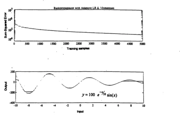
Figure 3.12 Function approximation using a two-hidden-layer network with 26 units in the 1st hidden layer, and 13 units in the 2nd hidden layer. Figure 3.13 Function approximation using a two-hidden-layer network with 40

units in the 1st hidden layer, and 20 units in the 2nd hidden layer. Figure 3.14 Function approximation using a two-hidden-layer network with 46

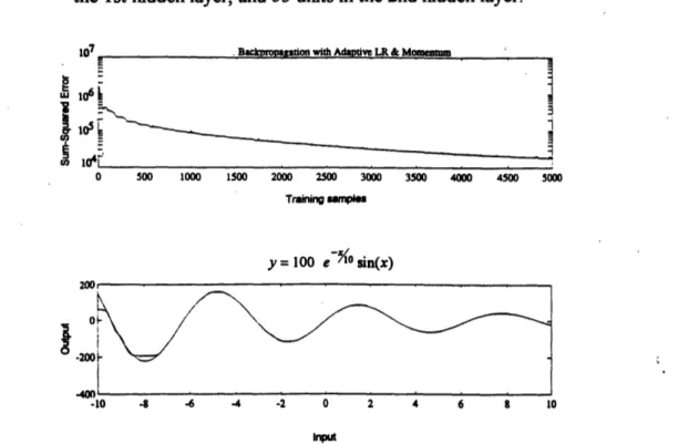
units in the Ist hidden layer, and 23 units in the 2nd hidden layer. Figure 3.15 Function approximation using a two-hidden-layer network with 53

units in the 1st hidden layer, and 27 units in the 2nd hidden layer. Figure 3.16 Function approximation using a two-hidden-layer network with 40

units in the 1st hidden layer, and 40 units in the 2nd hidden layer. Figure 3.17 Function approximation using a two-hidden-layer network with 27

units in the 1st hidden layer, and 53 units in the 2nd hidden layer. Figure 3.18 Function approximation using a one-hidden-layer network

with 80 units in the hidden layer.

Figure 3.19 Classification by two-hidden-layer networks. Figure 3.20 Cross-validation method.

Figure 3.21 A cantilever bending beam.

Figure 3.22 Noise-free and noisy input-output data. Figure 3.23 Effect of no. of units to approximation error.

Figure 3.24 Function approximation by a one-hidden-layer network. Figure 3.25 Performance of a one-hidden-layer network with 40 units.

Figure 3.26 Performance of a one-hidden-layer network with 60 units, which is initialized by a pretrained network with 40 units.

Figure 3.27 Performance of a one-hidden-layer network with 80 units, which is initialized by a pretrained network with 60 units.

Figure 3.28 Performance of a one-hidden-layer network with 80 units after being pretrained in Fig 3.27.

Figure 3.29 An example of a general RBFN.

Figure 3.30 Function approximation by RBFN with 10 Gaussian units. Figure 3.3 la Function approximation by MLN with BP,

with total no. of units of 50.

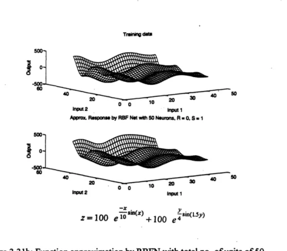
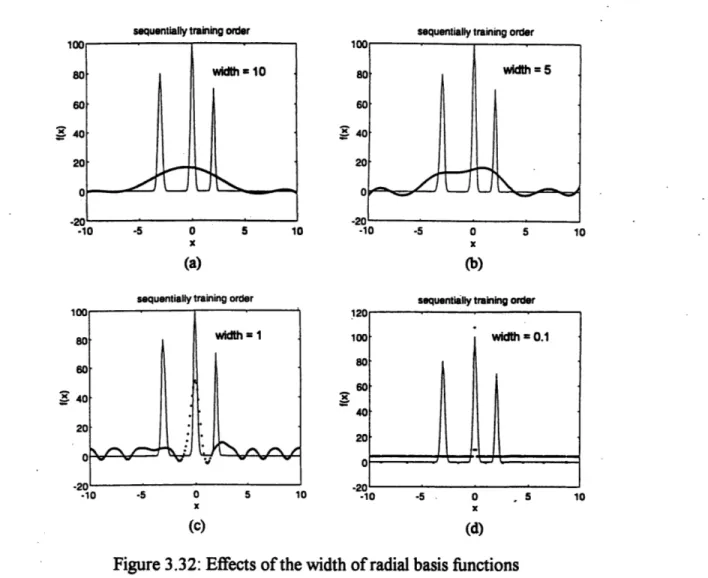
Figure 3.3 l1b Function approximation by RBFN with total no. of units of 50. Figure 3.32 Effects of the width of radial basis functions

on the approximation ability of RBFN.

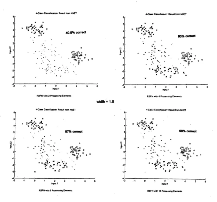
Figure 3.33 Effect of the no. of units on the classification ability of RBFN. Figure 3.34 Effect of the no. of units on the classification ability of RBFN. Figure 3.35 Effect of the width of radial basis functions to the classification

performance.

Figure 3.36 Effect of the width of radial basis functions to the classification performance.

Figure 4.1 A processing element. Figure 4.2 A simulated system. Figure 4.3 A simulated system.

Figure 5.1 A basic neural network-based diagnosis system.

Figure 5.2 The training process of neural network for detecting location of damage, NNET 1.

Figure 5.3 The training process of the neural network for recognizing the extent of damage.

Figure 5.4 Figure 5.5 Figure 5.6 Figure 5.7 Figure 5.8 Figure 6.1 Figure 6.2 Figure 6.3 Figure 6.4 Figure 6.5 Figure 6.6 Figure 6.7 Figure 6.8 Figure 6.9 Figure 6.10 Figure 6.11 Figure 6.12 Figure 6.13 Figure 6.14 Figure 6.15 Figure 6.16 Figure 6.17 Figure 6.18 Figure 6.19

The 2-span beam model.

Global and Global & Local structural diagnosis approach. General architecture of neural network-based diagnosis system. Global diagnosis system.

Global structure diagnosis, and Global & Local structure diagnosis, of a 2-span beam.

The 2-span beam model. General beam element.

Degree of freedoms of beam element no. 1.

Global degree of freedoms of the 2-span beam model. First 3 mode shapes of the unsymetrical 2-span beam. Data preprocessing approach.

A 1-hidden-layer networked used in damage diagnosis. Example of transfer functions.

Convergence of the training of an example network.

Significance of the no. of mode shapes to the accuracy of NNET1. Significance of the no. of points representing each mode shape to the accuracy of NNET1.

Significance of the no. of processing elements to the accuracy of NNET1.

Example of simulated acceleration response and its spectrums. Data preprocessing approach.

Effects of the location of sensors to the accuracy of NNET1. The significance of the no. of sensors to the accuracy ofNNET1. The significance of the no. of intervals to the accuracy of NNET1. The significance of the no. of hammers to the accuracy ofNNET1. The significance of the location of single hammer load.

Figure 6.20 Combination of locations of the 2-hammer case (1 hammer/span). Figure 6.21 Significance of the no. of processing elements to the accuracy

of NNET1.

Figure 6.22 Application on frame structures. Figure 7.1 A 4-span beam model.

Figure 7.2

General beam element.

Figure 7.3

Degree of freedoms of beam element no. 1.

Figure 7.4 First 3 modes of vibration of the 4-span beam model.

Figure 7.5

Data preprocessing approach.

Figure 7.6

The convergence of the Sum-Squared Error of the NNET1

of the global structural diagnosis.

Figure 7.7

The significance of the no. of mode shapes to the accuracy of

NNET1.

Figure 7.8 The significance of the no. of points representing each mode shape to the accuracy of NNET1.

Figure 7.9 The significance of the no. of processing elements to the accuracy of NNET1.

Figure 7.10 The significance of the no. of training samples to the accuracy of NNET1.

Figure 7.11 The acceleration response of DOFs 3 and 7, and their autospectrums, due to a hammer impulse.

Figure 7.12 Effects of the location of sensors to the accuracy of NNET1. Figure 7.13 The significance of the no. of sensors to the accuracy ofNNET1. Figure 7.14 The significance of the no. of intervals to the accuracy of NNET1. Figure 7.15 The significance of the no. of hammers to the accuracy of NNET 1. Figure 7.16 The effects of the location of sensors to the accuracy of NNET 1.

Figure 7.17 Figure 7.18 Figure 7.19 Figure 7.20 Figure 7.21 Figure 7.22 Figure 7.23 Figure 7.24 Figure 7.25 Figure 7.26 Figure 7.27 Figure 7.28 Figure 7.29 Figure 7.30 Figure 7.31 Figure 8.1 Figure 8.2 Figure A. 1 Figure B.1

The significance of the no. of processing elements to the accuracy of NNET1.

The significance of the no. of training samples to the accuracy of NNET1.

A middle span of a multi-span beam. A linear system.

Location of impulse generators for a middle span (2nd span). The first 3 modes of vibration of the 1st and 2nd span

of the 4-span beam.

The first 3 modes of vibration of the 3rd and 4th span of the 4-span beam.

The acceleration response and frequency transfer functions of DOF 14.

Data preprocessing approach.

The effects of the location of sensors to the accuracy ofNNET1. The effects of the number of sensors to the accuracy of NNET1. The significance of the no. of intervals to the accuracy of NNET1. The significance of the no. of processing elements to the accuracy of NNET1.

The significance of the no. of training samples to the accuracy of NNET1.

An example of a substructure of a frame and the local excitation. Example of multiple-point damage case and multiple-type

damage case.

Recommended approach for detecting unseen damage case. Modal analysis approach.

A linear system.

Transverse vibration of a beam with distributed load. Change of the 1st mode shape due to a damage condition. Change of the response spectrum of DOF 9 due to

a damage condition.

Transverse vibration of a beam with the bending moment at the left support.

Change of the frequency transfer function of DOF 3 due to a damage condition.

Figure B.2

Figure

C.1

Figure C.2

Figure C.3

Figure C.4

Figure

C.5

List of Tables

Table 1.1 Damage cases of the testing data set. Table 1.2 Damage cases of the training data set. Table 1.3 Damage cases of the testing data set. Table 1.4 Damage cases of the training data set. Table 3.1 The training time of feedforward networks.

Table 4.1 Types of transfer function for different neural network application. Table 6.1 The damage cases of the training data set.

Table 6.2 The damage cases of the testing data set. Table 6.3 The damage sensitivity of the optimum NNET1. Table 6.4 The damage sensitivity of the optimum NNET1.

Table 7.1 The basic damage cases for the global diagnosis system. Table 7.2 The possible combinations of damaged elements in

a particular span.

Table 7.3 The damage sensitivity of the optimum NNET 1. Table 7.4 The damage sensitivity of the optimum NNET1. Table 7.5 The damage sensitivity of the optimum NNET1. Table 8.1 The performance of optimized diagnosis systems. Table 8.2 The performance of optimized diagnosis systems. Table 8.3 The performance of optimized diagnosis systems. Table 8.4 The performance of optimized diagnosis systems. Table 8.5 The performance of optimized diagnosis systems.

Chapter 1

Introduction

1.1 Neural Network-Based Damage Diagnosis Approach

Although substantial research has been carried out on the topic of damage diagnosis of structures, the most reliable diagnostic techniques are still largely based on human expertise (DARPA, 1988). Since human-based structural damage diagnosis requires human experts to look for any signature that could identify damage of the structure, problems arise due to human errors and the scarcity of qualified human diagnosticians (Pham, 1995). There are also situations for which the human-based

approach is not practical such as damage diagnosis of structures in space, or structures in hazardous environments. Recently, the use of Knowledge Based Systems (KBS) to support human judgment has been proposed (DARPA, 1988 and Garrett, 1992), but this technology is also limited. Developing a KBS is very time-consuming (DARPA, 1988). Moreover, KBS's are not very adaptable and robust, and are too slow to be operated in real time (Pham, 1995). Therefore, a better non-human based approach is still needed.

By definition, a neural network consists of a number of units called " processing elements" which are connected to and interact with each other. The activation of a

network starts when there is input to any unit. The weighted summation of the inputs for a unit is passed through a function called "transfer function" and the output of this function is provided at the output connection, which can be connected to the input connection of

any other unit including itself. The activation process of each unit will continue to execute

until there is no more input, or until the output converges to some value. More details

about the architecture and operation of neural networks are presented in Chapter 2 and 3.

Considering the ability of artificial neural networks to approximate functions

(Cybenko, 1988, 1989; Hornik, 1989; Dyn, 1991; Park, 1991), the pattern mapping

aspect

of structural damage diagnosis appears to be a promising application area for neural

networks. If artificial neural networks can extract knowledge from remotely collected data

in an effective way, they can be incorporated in a computer based diagnosis system that

can complement existing human diagnosis approaches.

Neural network-based damage diagnosis approach has been studied recently by

several researchers. Elkordy (1992,. 1993), Rehak (1992), and Liu (1995) determine

changes in certain mode shapes of the damaged structure and use this information to

estimate the location and level of damage. Use of the frequency-domain properties of the

physical structure, referred to as the "vibrational signature" of the structure, transfers the

problem to static pattern mapping between changes in mode shapes and types of damage.

In this case, any type of network for function approximation (as discussed in Chapter 3)

can be applied to solve the mapping problem.

Elkordy (1992, 1993) trained a multilayer network with analytically generated

states of damage to diagnose damage states obtained experimentally from a series of

shaking-table tests of a five-story frame. The physical and analytical models are defined in

Fig 1.1. Damage states are simulated using a variety of smaller areas of bracing members

in the first two stories. Tables 1.1 and 1.2 contain the damage states of the testing and

training damage cases respectively. The performance of the neural network-based

diagnosis system that is optimized for the analytical model was examined and found to be

good for detecting a limited number of damage conditions of the real frame (see Table

'.4 cm

4 cm

4 cm

2 cm

Case Number Effective Bracing Area (cm2_{) Reduction of Bracing Area (%)}

First Floor Second Floor First Floor Second Floor

(b) Second Floor Damage Class

4 3.4 2.28 0 33 5 3.4 1.7 0 50 6 3.4 1.15 0 66 (c) Combined Damage 7 2.28 2.28 33 33 8 1.7 1.7 50 50 9 1.15 1.15 66 66 10 0.484 0.960 66 33

Table 1.1: Damage cases of the testing data set (Elkordy, 1992).

Case Number Reduction of Bracing Area (%) Target Diagnosisa First Floor Second Floor First Floor Second Floor

1 10 0 1 0 2 30 0 1 0 3 50 0 1 0 4 60 0 1 0 5 0 10 0 1 6 0 30 0 1 7 0 50 0 1 8 0 60 0 1 9 30 30 1 1 10 50 50 1 1 11 60 60 1 1

aKey: 1 = damage exists; 0 = no damage exists.

Using mode shapes to identify damage is only one approach. In the mechanical engineering field, vibrational response spectrums have long been used to detect damage of rotating tools and machines. This approach has been followed by Wu et al (1992) and MacIntyre et al (1994). Wu utilized a multilayer network to detect changes in the response spectrum of the numerical model of a 3-story shear building, and to correlate these

changes with corresponding damage states. The model is subjected to earthquake base acceleration, and the Fourier spectra of the computed relative acceleration time histories of the top floor are used in training the neural network. Damage is defined as a reduction of shear stiffness of a specific story. Only one story can be damaged at a time. The illustration of the model and data processing procedure are shown in Fig 1.2. Figure 1.3

shows the neural network employed for damage diagnosis. Tables 1.3 and 1.4 show the damage cases of the testing and training data sets respectively. The results indicate good performance of neural network in detecting damage of the model.

~uimu (wEwzuuuuj

3g

=

3l--•

¶

J1

.1

Accelrnadn ftm M

Cion eanhqupake

May 18, 1940 (SE compa..ne

Figure 1.2: The model and data processing procedure (Wu, 1992).

Damage tateI

0.0 0.5 1.0

I I I I I I I I

damage Activation value rep-resents the damage state of member 1

\

F

-no-ILdmag

Member 2 Member 3

Input layer MO nodesI

Fourier Spectrum

Figure 1.3: The multilayer network for damage diagnosis (Wu, 1992).

Case Number Reduction of Shear Stiffness (%)

1st Story 2nd Story 3rd Story

1 0 0 0 2 50 0 0 3 75 0 0 4 0 50 0 5 0 75 0 6 0 0 50 7 0 0 75

Table 1.3: Damage cases of the testing data set (Wu, 1992).

Case Number Reduction of Shear Stiffness (%)

1st Story 2nd Story 3rd Story

1 0 0 0

2 60 0 0

3 0 60 0

4 0 0 60

There are also other works that involve utilizing other vibrational signatures. Szewczyk and Hajela (1992, 1994) model the damage as a reduction in the stiffness of structural elements that are associated with observed static displacements under prescribed loads. They performed simulation of a frame structure model with nine bending elements and 18 degrees of freedom (X-Y displacements and rotation at each node). A variation of multilayer feedforward network was utilized to detect the damaged frame element. Barai and Pandey (1995) carried out a study on damage detection in a bridge truss model using multilayer network with simulated damage states, each represented by one damaged truss member. Discretized time history response at various locations of the truss due to a single-wheel moving load is used as the vibrational signature.

All of the research studies mentioned have been restricted to narrowly defined application areas. Issues related to the architecture and design strategy for a general neural network-based damage diagnosis system have not been addressed. Also, the efforts have focused on very small-scale problems that involve very limited number of possible damage states, and it is not obvious that the methods can be scaled up to deal with larger-scale problems. In most cases, at a particular instant in time, damage is assumed to occur at a single location (single-point damage condition) in order to reduce the complexity of the problem (Wu, 1992; Szewczyk and Hajela, 1994; Barai and Pandey, 1995). The treatment of multiple-point damage has been dealt with in a very limited way (Elkordy, 1992, 1993), and the methodology for dealing with multiple-point damage has not been adequately developed.

Based on our review of the literature, the important research issues concerning the applicability of neural networks for damage diagnosis that need to be addressed are as follows:

-_{The appropriate general architecture of a neural network-based structural}

- A comprehensive design strategy for neural network-based diagnosis system.

- The detection of simultaneous damage sources.

- The scalability of neural network-based diagnosis systems to large structures.

-The error introduced by representing the actual physical structure with an

ideological numerical model.

-

The choice of data such as. mode shapes, response spectrums, and other

vibrational signatures as input for damage classification.

-

The relationship between the data collection procedure and the performance of

the diagnosis system.

1.2 Objective and Scope

The primary objective of this research is to explore the potential of neural networks for structural damage diagnosis. To achieve this objective, a general neural network architecture for structural damage diagnosis and a methodology for designing the components of the architecture are formulated and evaluated.

The main components of the general architecture include i) the physical system of interest and its model ii) the data preprocessing units and iii) a collection of neural

networks that operate on the processed data and produce a prediction of the location and magnitude of damage. Important system design issues are the choice of variables to be observed, the methodology for choosing the excitation and type of vibrational signature

for the monitored structure, the actual configuration of the neural networks, and their training algorithm. These design issues are first examined in detail for the case of single-point damage condition, and the evaluation is then extended to the case of multiple-single-point

damage.

The evaluation phase is carried out with beam-type structures. As a first step, a single-point damage diagnosis system for a highly-idealized 2-span bending beam model is developed and evaluated. Two choices of excitation and vibrational signature are

considered. The first strategy applies ambient excitation to the numerical model of the structure, and then takes the mode shapes as input patterns for the neural networks which estimate the location and magnitude of damage. The second strategy applies a prespecified excitation to generate the model response, and employs the resulting response spectrum as input for the neural network system. The numerical modeling of the structure and the

computation of the response are carried out with MATLAB. Damage is introduced by reducing the bending resistance at a specific location. Simulation studies are performed to

evaluate the performance for the different choices of excitation and type of input. The second step in the evaluation phase considers a 4-span bending beam model with multiple-point damage. The diagnosis strategy is based on first identifying which

spans are damaged (global structural diagnosis), and then examining independently each individual damaged span to establish the location and extent of damage (local structural

diagnosis). Global structural diagnosis requires at least a set of neural networks for predicting which spans are damaged. Local structural diagnosis of each substructure requires at least two sets of neural networks for predicting the locations and extent of damage. The number of local structural diagnosis systems depends on the number of substructures.

Two choices of excitation and vibrational signature are employed for global structural diagnosis. The first choice uses ambient excitation to generate the response of the model, and takes the corresponding mode shapes as the input pattern for the neural

networks. The second choice employs a prespecified excitation and uses the corresponding response spectrum as the input pattern.

Local structural diagnosis employs a prespecified excitation to create the response of each substructure, and uses the frequency transfer functions of the substructure as input for the neural networks that perform damage diagnosis on the substructure.

Based on the results of the evaluation studies, a design methodology for a comprehensive neural network system for structural damage diagnosis is formulated. Results of additional studies on the performance of various configurations of multilayer feedforward network, with back propagation learning algorithm, are utilized to establish guidelines for the choice of appropriate configurations for the individual neural networks contained within the general architecture. Feasibility tests are also performed to explore the practical applicability of this diagnosis approach.

Two types of neural networks, one based on the multilayer feedforward-back propagation learning model and the other on radial basis functions, are appropriate for pattern classification. This study employed only the multilayer feedforward networks for the simulation studies since the lack of a-priori knowledge of the damage pattern mapping problem do not suit Radial Basis Function Network. Data on the performance of both types of networks is included in this document for convenient reference.

1.3 Organization

In Chapter 2, the basic concepts and definitions of artificial neural networks are described, several well-known architectures and training algorithms are demonstrated, and the neural network applications in civil engineering are briefly reviewed. Neural network and other information processing approaches, such as Knowledge Based Systems, are compared. The relation between neural networks and approximation schemes are also discussed.

Chapter 3 contains a detailed treatment of neural networks for function approximation, an application area of considerable interest for civil engineering.

Performance data are presented and discussed for both Multilayer Feedforward Networks and Radial Basis Function Networks. The optimum architectures and training strategies for a range of regression and classification problems are also investigated.

Feedforward neural networks, including Radial Basis Function Networks, are discussed in terms of probability and approximation theory in Chapter 4. Probabilistic models of feedforward networks with back propagation learning algorithms and radial basis function networks are investigated. This knowledge provides engineers with a different perspective of the theory of neural networks, and makes it easier to understand and develop a neural network-based system.

Chapter 5 is concerned with the application of neural networks to structural damage diagnosis. A general architecture of neural network for structural damage

diagnosis is presented, and methodologies for designing the individual components of the system for both single-point damage and multiple-point damage are proposed.

An application of a neural network based damage diagnosis system to a 2-span beam with single-point damage is developed and evaluated in Chapter 6. Chapter 7 describes the case of multiple-point damage diagnosis for a 4-span beam. These

investigations provide a general understanding of neural network based damage diagnosis and the difficulties involved in applying this approach to real structural problems. Chapter 8 summarizes these findings, and suggests strategies for overcoming some of these

difficulties. The practical applicability of this diagnosis approach is also discussed, and further research topics are recommended.

Chapter 2

Foundation of Artificial Neural Networks

2.1 Background History

Work in the neural network field began about 50 years ago. The effort during this time period can be considered to have three distinct phases (DARPA, 1987): an early phase, a transition phase, an a resurgent phase.

The early work, (1940's-1960's), was concerned with fundamental concepts of neural networks such as Boolean logic (McCulloch and Pitts, 1943), synaptic learning

rules (Hebb, 1949), single layer Perceptron (Rosenblatt, 1962), and associative memory (Steinbuch et al, 1963). The Perceptron generated immediate attention at that time

because of its ability to classify a continuous-valued or binary-valued input vector into one of two classes. However, in the late 1960's, the work by Minsky and Papert pointed out that the Perceptron could not solve the "exclusive OR" class of problems, and this finding

resulted in a substantial shift in research interest away from neural networks. During the transition period (1960's-1980's), a small group of researchers continued to develop a variety of basic theories that strengthened the foundation of the field. Contributions include the Least Mean Square (LMS) algorithm (Widrow and Hoff, 1960), Cerebellum model (Albus, 1971), competitive learning (Von Der Malsburg, 1986), and Adaptive Resonance Theory (Grossberg, 1987).

Starting in early 1980's, there was a resurgence in interest for neural networks. This resurgence was driven by the contributions made during the transition period toward improving the understanding of the deficiencies of single-layer perceptron and extending the theoretical work to multilayer systems. The advances in computer technology in the 1980's also provided the computation power needed to deal with large-scale networks. Notable contributions include feature maps classifier (Kohonen, 1982), associative memory theory (Hopfield, 1982), Boltzman machine (Hinton and Sejnowski, 1986), and Back Propagation learning algorithm (Rumelhart et al, 1986). These topics are described in more detail later in this chapter.

2.2 Topological Classification of Neural Networks

The word "neural" is used because the inspiration for this kind of network came initially from the effort to model the operation of neurons in human brain. Artificial neural networks are classified according to their topology and the algorithm that provides their ability to learn. The topology of an artificial neural network defines the connection between the various processing elements contained in the network. The function of a network is determined by its connection topology and the weighting factors assigned to each connection. These weighting factors are adjusted by the learning algorithm during the training phase. Artificial neural networks are also called "Connectionist Models", or

"Parallel Distributed Processing Models." For convenience, the simplified term "Neural Networks" is used throughout the remaining portion of this text.

Figure 2.1 shows a common processing element and its activation. A processing element has many input connections and combines, usually by a simple summation, the weighted values of these inputs. The summed input is processed by a transfer function which usually is a threshold-type function. The output of the transfer function is then passed on to the output connection of the element.

The output of a processing element can be passed on as input to any processing element, even to itself. Weights are used to designate the strength of the corresponding connections and are applied to the input signals prior to the summation process.

xo

lation

Figure 2.1: An example of a general processing element.

A neural network contains many "processing elements," or "units," connected and interacted to each other. Processing elements are usually clustered into groups called layers. Data is presented to the network through an input layer, and the response is stored in an output layer. Layers placed between the input and output layers are called hidden layers. When a network is not organized into layers, a processing element that receives input is considered to be an input unit. Similarly, a processing element that provides some output of the network is called an output unit. It is also possible that a processing element may act simultaneously as both input and output unit.

Based on topology, a neural network is classified as either feedforward or recurrent. Figure 2.2 illustrates these categories. Feedforward networks have their processing elements organized into layers. The first layer contains input units whose task is only to provide input patterns to the network. Next to the input layer are one or more hidden layers, followed by the output layer which displays the result of the computation.

In feedforward networks there is no connection from a unit to the other units in either previous layers or the same layer. Therefore, every unit provides information, or input,

only to units in the following layer. Since the input layer has no role other than to provide input data, it is not included in the layer count. It follows that an N-layer network has N-1 hidden layers and an output layer.

I1 2 Outout Output Hidden Layer 2 Hidden Layer 1 Input Buffer ....

F

Innut

r---a) Feedforward Network b) Recurrent Network

Figure 2.2: Feedforward network and recurrent network (Hertz, 1991).

Recurrent networks are networks that have connections "both ways" between a pair of units, and possibly even from a unit to itself. Many of these models do not include learning, but use a prespecified set of weights to perform some specific function. The network iterates over itself many cycles, until some convergence criterion is met, to produce an output. For example, the simplest recurrent network performs the following computation,

x(k+l = A x(k) , (2.1)

where x(k) is the output vector at time step k and A is a weighting matrix. The

convergence of this type of computation depends on certain properties of the weighting

2.3 Learning Algorithms

Learning, or training, is the process of adapting or modifying the connection weights and other parameters of specific networks. The nature of the learning process is based on how training data is verified. In general, there are 3 training categories;

supervised, unsupervised, and self-supervised.

Supervised learning requires the presence of an external teacher and labeling of the data used to train the network. The teacher knows the correct response, and inputs an error signal when the network produces an incorrect response. The error signal then

"teaches" the network the correct response by adjusting the network parameters according to the error. After a succession of learning trials, the network response becomes

consistently correct. This is also called "reinforcement learning" or "learning with a critic". Unsupervised Learning uses unlabeled training data and requires no external teacher. Only the information incorporated in the input data is used to adjust the network parameters. Data is presented to the network, which forms internal clusters that compress the input data into classification categories. This process is also called "self-organization." Self-supervised Learning requires a network to monitor its performance internally, and generates an error signal which is then fed back to the network. The training process involves iterating until the correct response is obtained. Other descriptors such as

"learning by doing", "learning by experiment", or "active learning" are also used to denote this approach.

Each learning method has one or more sub-algorithms that are employed to find the optimum set of network parameters required for a specific task. These sub-algorithms generally are traditional parameter optimization procedures such as least square

minimization, gradient descent, or simulated annealing. In more complicated networks, several types of learning algorithms may be applied sequentially to improve the learning ability.

Back propagation learning, the most popular for multilayer feedforward network, is a supervised procedure that employs a gradient descent type method to update the weighting parameters. With a gradient descent procedure, one updates parameters as follows:

W., = W, -. A Vf. (2.2)

where W is the vector of weighting parameters, f is the function to minimize (usually called an "error function"), and X is a parameter called "step size" or "learning coefficient." The advantages of this method are its simplicity and reliability. However, the method requires more computation than others, and also tends to lock in on local minima of the function surface rather than the global minima. The speed of convergence can be improved by varying the step size and including a momentum term. There are also improved gradient procedures such as Newton's method, Quasi-Newton, Conjugate gradient, and Stochastic Gradient Descent which is the stochastic version of the gradient method. The equation for Stochastic Gradient Descent has the following form

wn+

=

w-

(vf + s,).

(2.3)

where S is a sequence of random vectors with zero mean. Under certain assumptions, this sequence converges to a local minimum off (Girosi, 1993, 1995).

Although the stochastic version of gradient method is more likely to avoid a local minima, convergence to the global minimum is conditioned on certain assumptions. For instance, a particular stochastic method, called "Simulated Annealing" (Kirkpatrick et al,

1983), will converge to the global minimum with infinite updating. Stochastic methods are theoretically interesting, but they require extensive computation power and consequently their training time is too long for large-scale applications on current hardware.

The tasks which neural networks have to perform and the availability of training

data generally determine the appropriate type of training algorithm. In practice, there are

many criteria that have to be considered. Speed of training and degree of accuracy is

always a trade-off. Amount of available memory has to be considered when hardware is

restricted. In some case, even the characteristics of the error function have to be taken into

account. Having so many alternatives for the type of architecture and training algorithm, it

is difficult to find the right combination for a specific application. In most cases, a number

of candidate solution need to be evaluated in order to identify the best choice. This

research provides guidelines for selecting the proper architecture and training method for

function approximation. Details are presented in the next chapter.

2.4 Review of Types of Neural Networks

As mentioned earlier, neural networks are categorized by their architecture and learning algorithm. In this section some well-known networks are described in order to

provide further background for the neural network field.

Single and multilayer perceptrons are the simplest types of feedforward neural network model. The single-layer perceptron was first introduced by Rosenblatt (1962). An

example of the network is shown in Fig 2.3a. A processing element computes a weighted

sum of input, subtracts a threshold, and passes the result through a nonlinear threshold function,

fix)

(x) = 1 , x > 0 .

(2.4)

The two possible outputs correspond to the two different classes which can be recognized

by the network. The single-layer perceptron can be used to classify a continuous-valued or

binary-valued input vector into one of two classes. Training can be done with the Least

Mean Square (LMS) algorithm, which is a linear supervised training approach with guaranteed convergence. Minsky and Papert (1988) analyzed the single-layer perceptron and demonstrated that the network can only solve linearly separable problems like the exclusive AND problem, but cannot handle a nonlinearly separable problem such as the exclusive OR problem. A more detailed review of Rosenblatt's perceptron and Minsky and Papert's analysis can be found in (Minsky and Papert, 1988).

) =- •an(w • - tn, 01 Input layer Hidden layeri Outnut la•vr 1 '

(a) Perceptron that implement AND. (b) One-hidden-layer Perceptron Figure 2.3: Perceptron.

Multilayer perceptron is a feedforward network with one or more hidden layers. The transfer function of each processing element is the same as that of single-layer

perceptron. Although multilayer perceptrons perform better in many aspects compared to single-layer perceptrons, especially in their ability to solve nonlinearly separable problems, they were not very popular prior to the mid 1980's because of the lack of an efficient

training algorithm. The development of training algorithm called "back propagation" in the

mid 1980's (Parker, 1985; Rumelhart et al, 1986 and Werbos, 1974) resulted in renewed

interest in multilayer perceptrons. Back propagation is a supervised training procedure

that, although convergence is not guaranteed, has been applied successfully to many

problems such as spoken vowels classification (Huang et al, 1987 and Lippmann et al,

H1

1987), speech recognizer (Waibel et al, 1987), and nonlinear signal processing (Arbib,

1987). More details on back propagation are given in Chapter 3.

The Hopfield network is a one-layer unsupervised training recurrent network with

fully connected symmetrically weighted elements. Each unit functions as input and output

unit. In the initial version, all parameters had to be prespecified. This limitation is removed

in later versions where the parameters can be adjusted via gradient method such as Back

Propagation Through Time (Rumelhart et al, 1986), or Recurrent Back Propagation.

Given the input, the network iterates until it reaches a stable state (output from next

iteration does not change from the previous one), and provides the output. This type of

network can be used to solve pattern classification, associative memory, and optimization

problems.

(b)

(a)

Figure 2.4 Hopfield Network (Hertz, 1991). (a) Network architecture.

(b) The activation of the network for 4 time steps.

The optimization networks developed by Hopfield tend to converge to local

minima. The problem can be eliminated by adding a stochastic aspect to the training

algorithm during the iteration. This approach led to the development of a type of network

called "Boltzmann machine" (Ackley et al, 1985 and Hinton et al, 1986). The Boltzmann

machine training algorithm solved the credit assignment problem for the special case of recurrent networks with symmetrical connections and was demonstrated to be able to learn a number of difficult Boolean mappings. Due to the nature of stochastic parameter optimization, however, the training time of the Boltzmann machine is too long for most practical applications.

The Cerebellar Model Articulated Controller, or CMAC model (Albus, 1981), is an original model of the cerebellum, which is the part of the biological brain that performs motor control. The network adaptively generates complex nonlinear maps and is generally used in motor control problems such as robotic control (Kawato et al, 1987 and Miller et

al, 1987). CMAC is actually an adaptive table look-up technique for representing complex, nonlinear functions over multi-dimensional, discrete input spaces. A diagram of the

CMAC model is shown in Fig 2.5.

GENERATE RECEPTIVE STORED

FIELDS WEIGHTS

AND HASH CODING

Figure 2.5: The CMAC model (Albus, 1981).

CMAC reduces the size of the look-up table through coding, provides for response generalization and interpolation through a distributed topographic representation of

inputs, and learns the nonlinear function through a supervised training process that keeps adjusting the content or weight of each address in the look-up table (DARPA, 1987).

The feature map classifier (Hampson et al, 1987 and Valiant ,1985), as shown Fig 2.6, is a hierarchical network that utilizes both unsupervised and supervised training. The lower part of the network classifies the input and is trained first using Kohonen's feature map algorithm (DARPA, 1987), a type of learning algorithm that does not require explicit tutoring of input-output correlations and perform unsupervised training based on the input data. The perceptron-like upper part is then trained using a supervised training algorithm. This approach is especially useful when the amount of unsupervised training data available is significantly greater than the quantity of supervised training data.

SUPERVISED TRAINING

UNSUPERVISED TRAINING

Figure 2.6: A Feature Map Classifier (Hampson, 1987).

Adaptive Resonance Theory (ART) networks (Carpenter and Grossberg, 1987)

are complex nonlinear recurrent networks with an unsupervised training algorithm that

creates a new cluster by adjusting weights or adding a new internal node when an input pattern is sufficiently different from the stored patterns. "Sufficient difference" can be adjusted externally by a parameter called the "vigilance parameter". They are used mainly for pattern classification.

The Radial Basis Function Network (Broomhead and Lowe, 1988), or RBFN, is a 1-hidden-layer feedforward network with fixed nonlinear transformations in the hidden layer, and linear transformation in the output layer (see Fig 2.7). Radial basis functions are used as the transfer functions for the interior elements. The most popular choice of radial basis function is the Gaussian function

G,(x)

=

e

(2.5)

The output of RBFN is given by

n

y

XCG,(JJx-xll)

(2.6)

i=i

The type, the center points of the radial basis functions, and the weighting

parameters need to be specified. Since the gradient of the output error function is linear to weighting parameters, the error function does not have local minima and the weights can be adjusted by a linear optimization procedure such as a least square approach. These procedures converge rapidly to the global minimum of the error surface. This aspect makes RBFN an attractive alternative to MLN which requires a stochastic optimization procedure since its error function has local minima. More detail of RBFN is presented in Chapter 3.

Figure 2.7: A general Radial Basis Function Network.

2.5

Neural Network Applications

Examples of application of neural networks are: * Language Processing

-Text-to-Speech Conversion

* Image or Data Compression * Signal Processing

-Prediction or forecasting

- System modeling

-Noise filtering -Risk analysis

* Complex System Control

-Plant and manufacturing control

-Robotics control

-Adaptive Control

* Pattern Recognition and Classification

-Target classification

-Defect or fault detection

-Vision

- Symptoms-Source diagnosis * Artificial Intelligence

-Expert system

The tasks that neural networks are required to perform depend on the application area. Examples of different functions are:

-Prediction

Use input value to predict output value.

- Classification

Use input value to predict categorical output.

-Data Association (associative memory)

Learn associations of error-free or ideal data, then classify or associate data that contains error.

-Data Conceptualization

Analyze data and determine conceptual relationships.

-Data filtering

Smooth an input signal, reduce noise. - Optimization

Determine optimum value or choice.

Each application usually requires a different topology and learning algorithm. Chapter 3 discusses this aspect, mainly for networks that are employed to carry out

function approximation. A listing of the types of networks that are suitable for the various

tasks is given below.

Application Prediction Classification Data Association Data filtering Optimization Application Prediction Classification Association Conceptualization Data Filtering Optimization Network Type

multilayer network with nonlinear element, radial basis function network. multilayer network with nonlinear element, radial basis function network, recurrent network. multilayer network recurrent network recurrent network Supervised Training Yes Yes Yes No No No

There is no exact way to identify the best network or learning algorithm for a particular task. Different alternatives need to be evaluated. It may turn out that the optimum approach is to use a combination of several networks.

When the tasks are complex, it is usually better to divide these tasks into several less complex subtasks and develop separate networks for the subtasks. This approach is followed for the structural diagnosis application, and a detailed discussion is presented in Chapters 5 and 7.

2.6 Neural Networks in Civil and Environmental Engineering

Civil engineering applications of neural networks have become popular only since the late 1980's, after the work of Rumelhart (1986)1 revealed the potential of back

propagation learning algorithm. Researchers have utilized neural networks mostly for their regression and classification capability. Therefore, feedforward-type networks, mostly multilayer feedforward networks with a back propagation learning algorithm, have been the common choice since they are capable of performing well in both regression and classification. Some of the current applications of feedforward neural networks in Civil Engineering are described below (Garrett, 1992 and Pham, 1995):

- classification of distributed, noisy patterns of on-site information, such as classification of the level of cost for remediating hydraulic conductivity fields (Ranjithan, 1992), vehicle identification and counting applications (Bullock, 1991);

- interpretation of nondestructive evaluation sensory feedback, such as the use of neural networks in detecting the changes of response spectrums due to

structural damage (Wu, 1992), detecting flaws in the internal structure of construction components (Flood, 1994), or damage detection from changes in vibrational signatures in a 5-story model steel structure (Elkordy, 1993);

- modeling of complex system behavior, such as modeling complex material

constitutive behavior (Wu, 1991), modeling the behavior of large-scale structural systems for the propose of control (Rehak, 1992), modeling concrete material using actual experimental data (Ghaboussi, 1990), or predicting the flow of a river from historical flow data (Karunanithi et al, 1994);

- control of complex engineered facilities, such as the control of deflection of large-scale flexible structures (Rehak, 1992), or the control of an HVAC system for a large structure (Garrett, 1992).

In addition to the above applications, there are other civil engineering applications which employ recurrent or other feedback-type networks. These applications are mainly concerned with large-scale optimization problems such as resource leveling in PERT analysis for construction projects (Shimazaki et al, 1991).

2.7 Comparison of Neural Networks to Other Information

Processing Approaches

An expert system is constructed by first acquiring a human expert's way of solving a specific problem via extensive observation. This knowledge, or expertise, is analyzed and represented as rules which are embedded in a computer program. The construction of a neural network, on the other hand, starts by selecting an appropriate architecture and learning algorithm based on a priori knowledge of the problem. The networks are trained, either in supervised or unsupervised mode, with example data. The actual implementation of a neural network then can be done either with a computer program or a

specific-purpose hardwired device.

Although neural networks have been highly acclaimed as one of the most versatile approaches, it is unlikely that neural networks will replace either database processing or knowlegebase processing in the near future. Most likely, they will complement existing schemes in areas where their adaptability, ability to learn, and massive parallelism provides them with a significant advantage.

2.8 Relation of Neural Networks to Approximation Schemes

From another point of view, a neural network can be considered as a simple graphic representation of a parametric approximation scheme (Poggio and Girosi, 1991).

The network interpretation adds nothing to the theory of the approximation scheme, but it is useful from an implementation perspective. For example, its parallelism can take

advantage of parallel computing devices, and its modular form allows for sub-structuring to solve tasks.

Figure 2.8 shows a one-hidden-layer feedforward neural network that is a graphical representation of the following approximation scheme:

n

f*(4= cf(X.W) , (2.7)

i=1

which is known as the ridge function approximation scheme.

Similarly, the Radial Basis Function Network (see Fig 2.7) can be interpreted as the representation of the radial basis function approximation scheme,

f,*(4= cG(I

I

-

xII)

(2.8)

Both types of networks are discussed extensively in Chapter 3.=1 Both types of networks are discussed extensively in Chapter 3.

Y Y Y

Figure 2.8: A 1-hidden-layer feedforward network.

Approximation schemes have specific algorithms for finding the set of parameters that minimizes a prespecified function. These algorithms correspond to the learning algorithms of neural networks. For example, the back propagation learning algorithm can be considered as a version of the gradient method optimization approach combined with a specific credit assignment method. Similarly, the learning algorithm for RBFN is actually the least-square minimization approach.

Chapter 3

Neural Networks for Function Approximation

3.1 Introduction

Physical system modeling can be divided into two activities: performing regression to predict the system behavior, and performing classification to identify changes of

behavior. Regression involves mapping a numerical domain input to another numerical domain output, while classification maps a numerical or categorical domain input to a categorical domain output. Assuming that there is a function F that can perform regression or classification for the purpose of physical system modeling, approximating F can then be considered as a problem of system modeling.

As shown earlier in Chapter 2, networks that perform well in regression and classification are of the feedforward type such as the multilayer feedforward and radial basis function models. Although recurrent networks can also be used for classification, they are not considered here since they are based on unsupervised learning, whereas

structural damage diagnosis applications requires supervised learning. In this chapter, the performance of multilayer feedforward network for function approximation, a popular application in civil engineering, is discussed in detail. The performance of radial basis function networks is also investigated for the propose of providing a comparison. Extensive performance tests are presented to show the relative advantages and disadvantages of the multilayer feedforward networks versus radial basis function networks, and to identify their limitations for function approximation.