Application of high resolution remote sensing and GIS techniques for evaluating urban infrastructure

Application of High Resolution Remote Sensing and

GIS Techniques for Evaluating Urban Infrastructure

by

Lisa Yang

Submitted to the Department of Aeronautics and Astronautics in partial fulfillment of the requirements for the degree of Master of Science in Aeronautics and Astronautics at the

Massachusetts Institute of Technology

June 2018

2018 Massachusetts Institute of Technology. All rights reserved.

Author ...

Signature redacted

...

V

U

Lisa Yang Depart ent of Aeronautics and Astronautics

Signature redacted

May

Certified by ...

Olivier de Weck Professor of Aeronautics and Astronautics and Engineering Systems

Signature redacted

Certified by ...

Afreen Siddiqi Research Scientist, Institute of Data, Systems, and Society Thesis Supervisor

Accepted by ...

Signature redacted

MASSACHUSETS INSTrTUT E OF TECHNOLOGY

JUN

8 2018

LIBRARIES

Hamsa Balakrishnan Associate Professor of Aeronautics and Astronautics Chair, Graduate Program Committee

Application of High Resolution Remote Sensing and

GIS Techniques for Evaluating Urban Infrastructure

by

Lisa Yang

Submitted to the Department of Aeronautics and Astronautics on May 24, 2018 in partial fulfillment of the requirements for the degree of

Master of Science in Aeronautics and Astronautics ABSTRACT

City planners use information about a city's vegetation, urban morphology, and land-use to make decisions. The availability of high-resolution imagery is now expanding the type of information that can be used for planning as well as for understanding urbanization dynamics. This research uses very high resolution orthoimagery with three bands to obtain information about specific urban structures, such as roads and pavement, buildings, and solar panels, as well as non-impervious surface areas of vegetation and water. The maximum likelihood classifier (MLC) was used for the analysis of the images, and geographical information system

(GIS) techniques were used to extract features. Two case studies were done for the cities of

Phoenix, Arizona for the years 2004, 2006, 2008, and 2012 and for Seattle, Washington for 2002, 2005, and 2009. Results indicate that the area of buildings and the number buildings with solar panels have increased while the area of vegetation has increased for both Phoenix.and Seattle. The area of water has decreased for Seattle while the increase in water for Phoenix could suggest that more people are installing pools. The length of roads increases slightly for Seattle but decreases for Phoenix, a potential result of parking lots being converted into parking garages. The quantitative trends in the infrastructure were then compared to power law relationships between population and urban growing and scaling indicators.

Thesis Supervisor: Olivier de Weck

Title: Professor of Aeronautics and Astronautics and Engineering Systems Thesis Supervisor: Afreen Siddiqi

Title: Research Scientist, Institute of Data, Systems, and Society

Acknowledgements

This work would not have been possible without the financial support of the Y. T. Li fellowship from the Department of Aeronautics and Astronautics. I would like to express my gratitude to Professor Olivier de Weck for being my primary advisor and Dr. Afreen Siddiqi for being my advisor during Professor de Weck's sabbatical. Both have provided invaluable guidance and advice and shown me how to be a better researcher. I would also like to thank Madeline Wrable, a GIS specialist at the Rotch Library, for her assistance with ArcGIS and unending patience.

I would also like to thank my family and friends. They have always supported me

in whatever I pursue. To this end, they have been my rock and source of inspiration and fortitude. I am forever grateful for their love and support.

Contents

1 Introduction

1.1 M otivation and Organization . . . .

2 Literature Review

2.1 Remote Sensing Background . . . . 2.1.1 Obtaining Road Centerlines . . . .

2.1.2 Solar Panel Detection . . . .

3 Methodology

3.1 D ata . . . .

3.2 Image Pre-Processing . . . . 3.3 Segmentation using Mean Shift . . . . 3.4 Classification . . . . 3.4.1 Training Data . . . . 3.4.2 Maximum Likelihood Classification

3.5 Quantifying Urban Infrastructure . . . . .

3.5.1 Buildings . . . . 3.5.2 Vegetation . . . . 3.5.3 W ater . . . . 3.5.4 Road Lengths . . . . 3.5.5 3.6 Error 3.6.1 3.6.2

Number of Buildings with Solar Panel Installations . . A nalysis . . . .

Kappa Statistic for Assessing Classification Accuracy . Assessing Accuracy of Road Lengths . . . .

5 15 15 18 18 22 23 25 26 27 28 30 30 33 34 34 34 34 35 39 40 41 43 . . . . . . . .

3.6.3 Assessing Accuracy of Solar Panel Installations

3.7 Automation Using Python . . . . 44

4 Case Studies 46 4.1 Quantification of Urban Infrastructure . . . . 47

4.2 Error Analysis . . . . 54

4.2.1 Kappa Statistic . . . . 54

4.3 Length of Roads . . . . 58

4.4 Solar Panel Installation . . . . 59

4.5 Sensitivity to Tuning Parameters . . . . 59

5 Urban Growth and Sustainability 61 5.1 Scaling Relation as Urban Indicator . . . . 61

5.2 Traffic Delay . . . . 63

6 Discussion and Conclusion 65 6.1 Contributions . . . . 65

6.2 Limitations . . . . 66

6.2.1 Limitations Resulting from Images Themselves . . . . 66

6.2.2 Training Data . . . . 67

6.2.3 Computation . . . . 67

6.3 Future Work . . . . 67

6.3.1 Training Data . . . . 67

6.3.2 Use of Other Datasets . . . . 67

6.3.3 Use of Additional Datasets . . . . 68

6.3.4 Other Classification Algorithms . . . .. . . . . 69

6.3.5 Supercomputing . . . . 69

6 . . . . 44

List of Figures

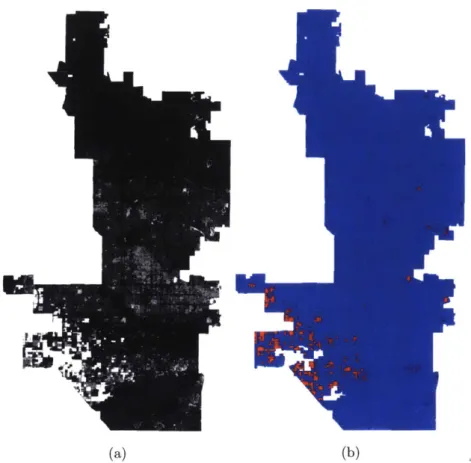
2.1 (a) LandSat image masked with Phoenix's city boundary and applied with

NDVI. (b) Threshold of 0.44 applied. Red pixels indicate vegetation. . . . . 20

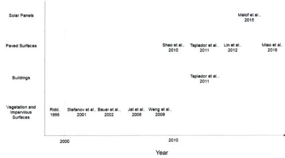
2.2 Summary of papers using remote sensing for urban applications. . . . . 21

2.3 Illustration of detecting center pixels for roads. Adapted from [48] . . . . 23

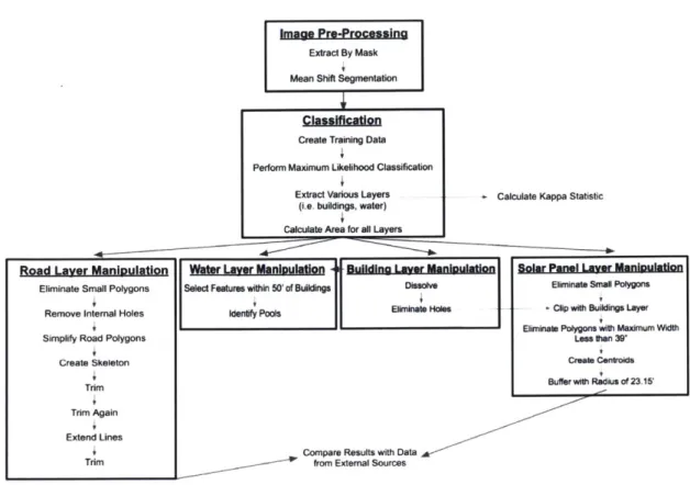
3.1 Summary of workflow used. . . . . 26

3.2 High resolution orthoimagery consisting of red, green, and blue bands. Adapted from [4]. . . . . 27

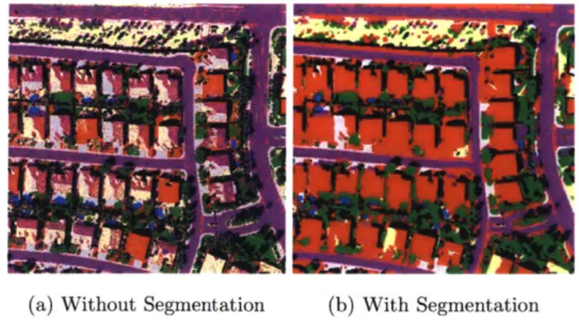
3.3 Classified images exhibit a "salt-and-pepper effect" without segmentation but show distinct boundaries with segmentation . . . . . 28

3.4 Seattle's sidewalks and roads are spectrally similar. Because sidewalks and roads were located close to one another, spatial detail and spectral values of 16 were used... ... 29

3.5 Illustration showing city boundaries and general areas from which training data was obtained and the Kappa statistic was tested. . . . . 32

3.6 Excerpt of signature file with mean values and covariance matrices used in clas-sification. . . . ... . . . . 33

3.7 Summary of work flow for obtaining length of roads. *See Figure 3.10 for more details... ... 35

3.8 Road sim plifying. . . . . 36

3.9 Example of how Thiessen Polygons are made. Adapted from [41]. . . . . 37

3.10 Work flow of how road centerlines, or skeletons, were obtained. Adapted from [3 8 ] . . . . 3 7 3.11 Road skeleton post-processing to obtain final road centerline. . . . . 38

Summary of work flow for obtaining number of buildings with solar panels. . Buffer analysis to determine number of buildings with solar panels. . . . . Confusion or error matrix for calculating Kappa statistic. Adapted from [14]. 4.1 Location of Phoenix, Arizona and Seattle, Washington in the United Stat 4.2 Area of buildings per year for Phoenix .. . . . .

Area of vegetation per year for Phoenix. . . . . Area of water per year for Phoenix .. . . . . Number of buildings with solar panels per year for Phoenix. Length of roads per year for Phoenix. . . . .

Population per year for Phoenix. . . . . Area of buildings per year for Seattle. . . . . Area of vegetation per year for Seattle. . . . . Area of water per year for Seattle. . . . . Number of buildings with solar panels per year for Seattle. . Length of roads per year for Seattle. . . . . Population per year for Seattle. . . . . Examples of false detections of solar panels. . . . .

es. . . 46 . . . . 48 . . . . 49 . . . . 49 . . . . 50 50 . . . . 51 . . . . 51 . . . . 52 . . . . 52 . . . . 53 53 . . . . 54 57 8 3.12 3.13 3.14 39 40 42 4.3 4.4 4.5 4.6 4.7 4.8 4.9 4.10 4.11 4.12 4.13 4.14

List of Tables

2.1 Most often used remote sensing satellites. Adapted from [13]. . . . . 19

2.2 Features extracted from each region. Adapted from [17]. . . . . 24

3.1 Table summarizing metadata for Phoenix and Seattle. . . . . 27

3.2 Table summarizing parameters used for mean shift segmentation in ArcMap. . 30 3.3 Classes defined for classification. . . . . 31

3.4 Degree of automation and estimation of how long each process took. . . . . 44

3.5 Manually selected parameters used in this study. . . . . 45

4.1 Classification accuracy results for Phoenix, AZ. . . . . 55

4.2 Classification accuracy results for Seattle, WA. . . . . 56

4.3 Table showing results for error analysis for road lengths. . . . . 58

4.4 Table showing results for error analysis for number of buildings with solar panels. 59 4.5 Table showing results for various parameter values. Columns 1-4 show parame-ters' names, current values used for the parameters in this research, which new values were tested, and percent change. Columns 5-8 show quantification of urban infrastructure as a result of the parameters. . . . . 60

5.1 Scaling indicators for Phoenix and Seattle. Note that "Water" for Phoenix includes all water surfaces. . . . . 62

5.2 Table showing values for population, length of roads, and traffic congestion for P hoenix . . . . 63

5.3 Table showing values for population, length of roads, and traffic congestion for S eattle. . . . . 63

5.4 Table showing / and y values relating road lengths and population to traffic congestion. . . . . 64

List of Acronyms, Abbreviations,

and Variables

a

Ae Set of Canny edges for road extraction

A Percent area of class i AZ Arizona

B Number of bands

Br Metabolic rate

,3 Exponent value reflecting relationship between population and material resources

C Cluster number for EM clustering algorithm for road extraction

c Confidence interval

Ck Covariance matrix for class k |Ck| Determinant of Ck E Allowable error EM Expectation maximization Ek Canny edge ft Feet 11

f(x)

f (X

Exponent relating road lengths and traffic congestion Geographic information system

Inches

Impervious surface area Kernel

A Class in MLC Kappa statistic

Kappa statistic weighted with area LandSat Multispectral Scanning System LandSat Thematic Mapper

Neighboring pixels pixels for road centerline extraction Largest pixel in search window for road centerline extraction Light Detection and Ranging

Likelihood used in MLC Logistic model tree Logistic Regression

Linear spectral mixture model Number of endmembers for LSMM Number of rows in an image

Meters Body mass

MPV RGB Multivariate normal probability distribution

MLC Maximum Likelihood Classification MSER Maximally Stable Extremal Region

N Sample size

n Number of columns in an image

NDVI Normalized Difference Vegetation Index

rne Weighted summed row totals for calculating weighted Kappa statistic

ni+ Row totals or number of sample points classified into class i for calculating the Kappa statistic

NIR Near infrared band

nj+ Column totals or number of sample points classified into class

j

N(t) Population at a given time

p Number of features, usually bands

pc Gaussian distribution density for EM clustering algorithm for road extraction

pi

P(k) Prior probability of class k P(Xlk) Conditional probability of class k

p(x) Kernel density estimate for mean shift segmentation r Noise in LSMM

RF Random Forests

Red Red band

RGB Red, green, and blue bands of an image

S Spectral signatures of M endmembers

a Bandwidth

E, Covariance matrix of pc

SGB Stochastic Gradient Boosting

Spi Slope around pi sq ft Squared feet

SVM Support vector machine T Trace operation

TIR Thermal infrared

TOA Top of the atmosphere

p, Mean of pc

Ilk Vector of mean values for class k u Expected percent accuracy

UHI Urban heat island

USGS United States Geological Survey

V-I-S Vegetation-impervious-soil

WA Washington

wC Weight of cluster C Xregion 3-dimensional RGB value

y Low-resolution image used in LSMM

Y Constant in power law relationship for describing how a city's resources grow

Y(t) Material resources or amount of social activity at a given time

Z Z-value from standard normal distribution

Chapter 1

Introduction

1.1

Motivation and Organization

Today's cities are growing in size and number. In 2016, 512 cities had at least 1 million residents, and 23% of the world's population lived in a city with at least 1 million inhabitants [43]. It is projected that by 2030, 662 cities will have at least 1 million residents and 27% of the world's population will live in cities with at least 1 million residents [43]. As urbanization proceeds rapidly, there is a growing desire to understand how urbanization impacts urban sprawl [22], urban heat island effect (UHI) [21, 30, 11], quality of life [9], and other broader, environmental factors such as biodiversity [42].

Since cities are centers of human activity, urban mapping is becoming more important. The objective of urban mapping is to accurately describe the figure, structure, geography, and relationships of a city's features [10]. Traditional methods based on field investigations, surveying, and mapping techniques are time-consuming and expensive and cannot keep up with the pace of urban development. In addition, data acquired through traditional methods is sometimes not available or even attainable, like in the situation with developing countries. Because of this, remote sensing has become useful for the monitoring and prediction of urban growth. Remote sensing is widely used among urban planners and policy makers as a tool for extracting urban information such as vegetation distribution, urban morphology, and land-use mapping [13]. In addition to using remote sensing for studying land-use in a single city, remote sensing is also helpful in comparing data across various cities. Data collected by local agencies

using human social processes could be biased because of local assumptions, nomenclature, etc. Remotely sensed data can be a transparent, reliable source to compare cities.

Thermal infrared data (TIR) has been widely used to obtain land surface temper-ature (LST) [21, 30, 11]. LST is an important parameter when studying the urban thermal environment and the effects of UHI. TIR data is available from a series of satellite and air-borne sensors; one widely available TIR dataset is Landsat. TIR sensors measure top of the atmosphere (TOA) radiances which can be converted into brightness temperatures [31]. Un-derstanding where high LST values are located within a city helps city planners determine where to potentially add more vegetation, for example, to mitigate UHI.

A city's impervious surface area (ISA) is another parameter that measures urban

growth and density. ISA is the area consisting of human-made surfaces: residential, commer-cial, and industrial structures like buildings, paved roads, etc. There have been several studies that quantified ISA using remotely sensed data in various cities across the globe [20, 46, 31, 22]. These studies used Landsat data where the resolution was 30 meters.

With high-resolution remote sensing data becoming more publicly available, there are opportunities to gain new information about urban change, urban sustainability using new measures of infrastructure (road networks, swimming pools, etc.) and technologies (solar panels, etc.) In this research, an attempt was made to investigate the usefulness of spatial techniques for urban structures, such as roads, buildings, and solar panels, as well as non-impervious surface areas like vegetation and water. The growth in road network, solar panel installations and increases in vegetation and water in the cities of Phoenix, Arizona and Seat-tle, Washington were estimated using very high resolution orthoimagery. A statistical image classification method, the maximum likelihood classifier, was used for the analysis of the im-ages. Once the images were classified, geographical information system (GIS) techniques were used to extract features.

The thesis is organized in the following way:

" Chapter one includes the motivation for this research.

" Chapter two provides a literature review of topics closely related to this topic.

* Chapter three discusses the methodology used in this study to extract and quantify the area of vegetation and water, the length of road networks and number of solar panel

installations, as well as the methods used to assess the accuracy of these values.

" Chapter four presents case studies for Phoenix, Arizona and Seattle, Washington using

the methods in chapter three. Results for the quantification of certain urban infrastruc-ture and error analysis are presented.

" Chapter five relates results presented in chapter four to urban growth and sustainability

models.

" Finally, chapter six includes a final discussion of the merits of this work, including

strengths, limitations, and how this work can be improved through future work.

Chapter 2

Literature Review

2.1

Remote Sensing Background

Remote sensing gathers information from distant objects by measuring radiation that the objects reflect or emit. Remote sensing began as early as the 1800's when Gaspard Tournachon captured the first recorded aerial photograph from a balloon [28]. By the 1970's, the first Earth observation satellite, more commonly known as LandSat, was launched. The first generation sensors on the LandSat Multispectral Scanning System (LandSat MSS) satellites were able to produce images with a spatial resolution of 80 meters per pixel and had a temporal resolution, or revisiting time, of 18 days. In 1986, second-generation satellites, like the LandSat Thematic Mappers (LandSat TM), improved spatial resolution to 30 and temporal resolution of 16 days. Near the end of the 1990's, third-generation satellites like Ikonos were launched and had very high spatial resolution of 5 meters per pixel and temporal resolution of 1.5 days. Table 2.1 summarizes some of the most often used remote sensing satellites. As indicated, over the years, the spatial and temporal resolutions improve.

Table 2.1: Most often used remote sensing satellites. Adapted from [13].

System Spectral resolution Spatial resolution (pixel size -meters) Temporal resolution (days) Archive since

Landsat MSS 3 bands visible 80 18 1972

1 band infrared 1 band thermal infrared

Landsat TM 3 Bands visible 30 - Visible and infrared 16 1986

3 Bands infrared 60 - Thermal infrared 1 Band thermal infrared

Landsat ETM+ 3 Bands visible 30 - Visible and infrared 16 1999

3 Bands infrared 60 - Thermal infrared 2 Bands thermal infrared 15 -Panchromatic

I Band panchromatic

SPOT 1 2 Bands visible 20 -Visible and infrared 26 1986

SPOT 2 1 Band infrared 10 - Panchromatic

SPOT 3 1 Band panchromatic

SPOT 4 2 Bands visible 20 -Visible and Infrared 2-3 1998

2 Bands infrared 10 - Panchromatic

I Band panchromatic

SPOT 5 2 Bands visible 20 - Mid infrared 2-3 2002

2 Bands infrared 10 - Visible and near infrared I Band panchromatic 2.5-5 - Panchromatic

ASTER 3 Bands visible 15 -Visible 16 1999

6 Bands infrared 30 - Infrared 5 Bands thermal infrared 90 - Thermal infrared

IRS-1C 2 Bands visible 23.5 -Multispectral 5-24 1995

2 Bands infrared 5 -Panchromatic I Band panchromatic

Ikonos 3 Bands visible 4 - Multispectra) 1.5-2.9 1999

1 Band infrared 1 - Panchromatic

Quickbird 3 Bands visible 2.4 - Multispectral 1-3.5 2001

1 Band infrared 0.6 - Panchromatic

1 Band panchromatic

Since remotely sensed images cover a wide area and can revisit the same location, remote sensing is a way to observe urban change and test models. Traditionally, within the realm of urban applications, remote sensing has been used to assess land cover and land usage. Numerous studies have investigated the cover of impervious and non-impervious surfaces within a city. Ridd [23] used the vegetation-impervious-soil (V-I-S) model to identify various biophysical parameters in an urban ecosystem, such as moisture, vegetation, and the impact on human responses. Similarily, Bauer et al. [20] and Stefanov et al. [46] quantified impervious surfaces in various cities using LandSat data.

(a) (b)

Figure 2.1: (a) LandSat image masked with Phoenix's city boundary and applied with NDVI.

(b) Threshold of 0.44 applied. Red pixels indicate vegetation.

At the beginning of this study, an attempt was made to use LandSat data to ob-tain information about vegetation, water, impervious surfaces, and other land coverage in an urban environment. Figure 2.1a shows an example LandSat image that was masked using Phoenix's city boundary. The Normalized Difference Vegetation Index (NDVI) was used to show vegetation:

NDVI = NIR - Red (2.1)

NIR + Red

where NIR is the near infrared band and Red is the red band. NDVI values range from -1 to

1, and whiter pixels indicate NDVI values closer to 1 and thus are more likely to be vegetation.

Next, a threshold based on the histogram of pixel values was applied. Figure 2.1b shows the resulting image with a threshold of 0.44. The red pixels indicate vegetation. However, it was quickly determined that obtaining information about detailed urban land coverage like roads

and houses would not be possible using indices and LandSat image. Another option, one with higher resolution, was needed.

In recent years, high resolution images have been classified to identify a city's green areas, water bodies, paved streets, bare soil, and buildings. Tapiador et al. [6] used a neural network classifier to determine the relationship between the availability of green areas, sport facilities, private swimming pools, and pavement in Lima, Peru. Similarly, very high resolution imagery have been used to assess inner-city growth by detecting new buildings within neigh-borhoods using object-based approaches [8]. Some work has also been done in road extraction [48, 49, 45] and solar photovoltaic panel detection [17] from remotely sensed imagery. Figure 2.2 summarizes some key papers that have used remote sensing for urban applications. Be-cause of the increasing availability of high-resolution and very high-resolution images, remote sensing analysis for the urban environment has trended towards finer resolution objects. The following sections in the chapter will discuss methods used to obtain information about roads and solar panels using remote sensing.

Solar Panels Malof at al.,

2015

0

c Paved Surfaces Shao St al., Taplador et al., Un at al., Miao et al..

O 2010 2011 2012 2016

Buildings Taplador at al.,

2011

Vegetation and Ridd, Stefanov et al.. Bauer et al.. Jat et al., Weng et al.,

impeus 1995 2001 2002 2008 2009

2000 2010

Year

Figure 2.2: Summary of papers using remote sensing for urban applications.

2.1.1 Obtaining Road Centerlines

Information of road networks can assist urban expansion estimation and the monitoring of traffic and population movement. To this end, obtaining road networks from remotely sensed images has become popular recently.

Extracting Road Segments

Miao et al. [49] uses expectation maximization (EM) clustering to extract road segments. The multispectral image is first divided into non-overlapping regions using the EM clustering algorithm for segmentation. In the EM clustering algorithm, the image is a set of vectors

X1, X2, ...XN in a d-dimensional space from a Gaussian mixture:

C

p(x; pc;

)

C c=1

Pc(X) = 1 exp { (X - [)T(Z )(X - tt)} (2.3)

2741I

EC

where C is the cluster number, pC is the Gaussian distribution density with mean p, and covariance matrix

EC,

we > 0 (2.4)

C

We = 1 (2.5)

C=1

Other road extraction methods include the detection of Canny edges. As shown by Lin and Tseng [45], a set of Canny edges, Ae, is denoted as:

Ae = {Ek(2.6)

where Ek is a Canny edge represented as a set of connected edge pixels, pi:

Ek= {Pi}I.k1 (2.7)

Road Centerline Extraction

Shao et al. [48] assumes that the center pixel and its neighboring pixels have lighter grey values than the surrounding pixels. In order to detect road center points, the following algorithm is used:

1. For a pixel Pi and its neighboring Lb - 1 pixels, obtain the biggest Le pixels out

of all pixels in the search window and store them into a set S,,(i) = 0, ... , Le - 1

2. Compare two pixel windows S,, and T. If Tw(k) E S, where k = 0, ... , Lb - 1,

the pixel Pi is the center point. Figure 2.3 illustrates this two-step algorithm.

Original one dimensional Image profile

P, 1681701721741761791821131801811781751731711691. 0 1 2 Lb-3 Step 1: constructing T, nd S. L=15 33 82 81 80 79 78176175174173 72171170169168 r,=5

Step 2: if T.(k)e S. the pixel Pj is judged as a center pixel

Figure 2.3: Illustration of detecting center pixels for roads. Adapted from [48]

Then, lines whose length is less than a pre-determined threshold were removed to eliminate false roads. As mentioned by the authors, determining an appropriate threshold is difficult.

Another method of extracting road centerlines is use Canny edges presented in [45]. For each pixel pi, the slope S,, around pi is determined by fitting a line with some neighbors of pi. Then, a perpendicular line to S, is calculated. The dot at pi is extended in the perpendicular direction until it reaches both of the Canny edges. By connecting these center dots, a center line can be obtained.

2.1.2 Solar Panel Detection

Malof et al. [17] presents a methodology of identifying solar panels in Lemoore, California using very high resolution satellite orthoimagery. One hundred different houses, totaling 0.196 square kilometers, were chosen for the dataset. The first fifty houses had solar panels while the second fifty houses did not. For training, polygons were drawn around all of the rooftop solar panels. Pixels were clustered into regions, and Maximally Stable Extremal Regions

24

(MSERs) are identified and eliminated, resulting in removing 30% of the regions with the lowest confidence intervals c:

c = logP(XregionjMPVRBG) (2.8)

where Xregion is the 3-dimensional mean red, green, and blue (RGB) value in each region, and MPVRGB is a multivariate normal probability distribution with mean and covariance parameters determined from the hand-selected truth regions during the training phase.

Table 2.2: Features extracted from each region. Adapted from [17].

FeatureFeature

Space

Feature Feature description Fetr ipc

name Dimen__onalty

Foreground Prescreener confidence, c I

color

Background _{First 10 principal components of 3-D 10} color color histogram of background pixels

Shape Perimeter length, ₂

features 1 Extent = Area/BoundingBoxArea

Shape Compactness = Area/Perimeter2_{, 2}

features 2 Solidity = Area/BoundingArea

Texture _{Mean, Variance, and Kurtosis of 3}

features grayscale pixels within region

Next, a machine learning classifier was used assign a new statistic to each region using feature processing. Table 2.2 shows the features extracted from each region. Using these features, a support vector machine (SVM) classifier is used to classify each region. Finally, mean-shift segmentation is performed to combine any regions that are located very close to each other.

One limitation of this approach is that classification was performed on and evaluated with the data that was trained. As a result, naturally, classification will perform better. However, this methodology can be applied to investigate rooftop solar panels for an entire city.

Chapter 3

Methodology

An object-oriented approach was used in this study. The two main functions were image segmentation and classification. Once classification was complete, further processing using various methods was done to quantify selected variables. Finally, error analysis was done to demonstrate the accuracy of these processes. Esri software including ArcMap and ArcGIS Pro were utilized in this study, and Python was used to automate several processes. Figure 3.1 illustrates the workflow used in this research. More details for each block will be addressed in the coming sections.

Image Pre-Processing

Extract By Mask

Mean Shift Segmentation

Classfficatoln

Create Training Data

Perform Maximum Likelihood Classification

Extract Various Layers + Calculate Kappa Statistic (i.e. buildings, water)

Calculate Area for all Layers

Road Layer ManiDulatlon Wl L Manipulatn Building Ljr Manilulation Solar Panel Layer Manipulation

Eliminate Small Polygons Select Features wIthin 50'of Budings Dissolve Eiinate Small Polygona

Remove Internal Holes kentily Pools

Eliminate Polygons with Maximum Width

Simplify Road Polygons Laos OW 39"

Create Skeleton Create Centrols

Trim Buter with Radius of 23.15'

Trim Again

Extend Lines

Compare Results with Data

Trim from External Sources

Figure 3.1: Summary of workflow used.

3.1

Data

Aerial, high resolution orthoimagery was obtained through Earth Explorer, an online database from the United States Geological Survey (USGS), and covered the span of the geographic area of interest and for the desired time frame. These images consisted of the red, blue and green bands, each captured at its respective wavelength. Each band is a raster dataset of pixel values which are used later in segmentation and classification. Figure 3.2 illustrates the bands that comprise the high resolution orthoimagery. Table 3.1 summarizes the metadata.

27

Red Band

MA-1 Green Band

Blue Band

High Resolution Orthoimagery

Figure 3.2: High resolution orthoimagery consisting of red, green, and blue bands. Adapted from [4].

Table 3.1: Table summarizing metadata for Phoenix and Seattle.

Phoenix, AZ 2004 Sept 1, 2004 -Sept 1, 2004 708 0.25 m 2006 Sept 1, 2006 -Sept 1, 2006 622 0.8 ft 2008 Nov 1,2008-Jan 1, 2009 558 0.8 ft 2012 Sept 1,2012-Dec 31, 2012 559 0.8 ft

NAD83NAD83 NAD83 NAD83

Zone 12N _{Zoe 2N Central (ff)} Arizona _{Central (ft)} Arizona _{Central (ft)}Arizona

2002 June 2, 2002 -June 20, 2002 136 0.3 m Seatfle, WA 2005 Aug 1, 2005 -Aug 1, 2005 66 2009 May 28. 2009 -May 30, 2009 137 0.3 m 0.3 m

NAD83 UTM NAD83 UTM NAD83 UTM

Zone ION Zone 1ON Zone 1ON

3.2

Image Pre-Processing

Since the images' extent fell outside of a city's boundary, images were pre-processed so that only images or parts of images located within the city limit would be considered. Phoenix's and Seattle's city boundaries were obtained from their local GIS departments [15, 33]. Phoenix's city limits were modified so that any internal holes were removed. Seattle's city limits were

28 Year Acquisition Date Number of Images wilin CitY Rmo Presolution

modified to include the western and eastern boundaries since the original file only included the northern and southern boundaries. Figure 3.5 shows both cities' boundaries, which were used to clip images using the Extract By Mask tool in ArcMap. The boundaries were also used to calculate each city's area which is used in future calculations.

3.3

Segmentation using Mean Shift

Because this study includes the extraction of objects like roads and solar panels, segmentation was performed to segment images into non-overlapping clusters. Segmentation is a process that identifies group of adjacent pixels, sometimes referred to as superpixels, that have similar spectral characteristics. Rather than performing classification on individual pixels, classifi-cation was done on these segments or superpixels. Figure 3.3 shows the "salt-and-pepper" effect when segmentation is not used (left) and distinct boundaries when segmentation is used

(right).

(a) Without Segmentation (b) With Segmentation

Figure 3.3: Classified images exhibit a "salt-and-pepper effect" without segmentation but show distinct boundaries with segmentation.

Images were segmented using the mean shift algorithm, a method of clustering. The following derivation is from [19]. The kernel density estimate, a generalization of histograms defining density estimates, is defined as:

N

p(x) =- K(11 x X 12), x E R D (3.1)

with {xi}n_ 1 being the data points to be clustered, bandwidth o- > 0, and kernel K. Using an

iterative scheme x+1 f(x') to obtain a mode, or local maximum of density, of p:

N K'(11|-*i||2₎

(3.2)

f (X) = EN K( -My. 112)

j=1 j=1 K(I0, II 2)

From this, the mean shift is f(x) - x.

The mean shift algorithm is utilized in ArcMap's tool Segment Mean Shift, used to segment the images. In addition to the images, this tool also uses spectral and spatial detail values ranging from 1 to 20 to smooth the images. A higher spectral detail value is used when cluster will have somewhat similar spectral characteristics while a higher spatial detail value is used when clusters are closer together [34]. Since some of the classes, like houses and bare earth, used in the classification step are quite similar, a spectral detail value of 15 was used. Because roads and buildings are somewhat close to one another, a higher spatial detail value is desired. Due to computational limits and the large number of images, a spectral detail value of 10 was used for Phoenix.

W,,

Figure 3.4: Seattle's sidewalks and roads are spectrally similar. Because sidewalks and roads were located close to one another, spatial detail and spectral values of 16 were used.

Seattle's features that were spectrally similar were much closer to one another than those of Phoenix. For example, Seattle's sidewalks and roads, which are located near each other, appear very similar as shown in Figure 3.4. Because of this, and the fact that the datasets for Seattle contained fewer images (i.e. less computational time), a spatial detail and

spectral values of 16 were used. Table 3.2 summarizes the parameters used for mean shift segmentation for each city.

Table 3.2: Table summarizing parameters used for mean shift segmentation in ArcMap.

Phoenix, AZ Seattle, WA

Spatial Detall 10 16

Spectral DetaIl 15 16

3.4

Classification

Image classification includes determining a priori the number and characteristics of the classes within the extent of the images and assign labels to pixels based on their properties using some sort of classification scheme. There are two main approaches to classification and labeling: supervised and unsupervised. This study uses supervised classification. The various steps such as selecting training samples and using Maximum Likelihood Classification (MLC) are addressed in this section.

3.4.1 Training Data

Supervised classification is characterized by using prior knowledge of what pixels make up the image. Statistical characteristics of the image are estimated from the training samples provided

by the user. Obtaining appropriate training data that accurately represents the rest of the

image as a whole can often be challenging since the accuracy in classification depends on the representativeness of the estimates of the number of training samples, the statistical nature that results from these samples, and the size of the sample [reference to Computer Processing of Remotely Sensed Images]. For sample size, a general rule of thumb is to use at least 30p pixels per class, where p is the number of features like spectral bands [27]. However, depending on the classes that are being trained and classified, it is often beneficial to use more samples to ensure that all types of surfaces and pixels are being considered.

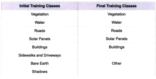
Table 3.3: Classes defined for classification.

Initial Training Ciasses Final Training Classes

Vegetation Vegetation

Water Water

Roads Roads

Solar Panels Solar Panels

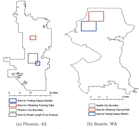
Buildings Buildings

Sidewalks and Driveways

Bare Earth Other

Shadows

In this study, a training data set containing the categories shown in the first column of Table 3.3 were created for each year of analysis for both Phoenix and Seattle. The initial classes in the training data were roads and other pavement surfaces, buildings, vegetation, water, solar panels, sidewalks and driveways, bare earth, and shadows. The latter three classes were combined into a class named "other" since they were not the focus of this study. Table

3.3 shows some examples for each class.

The area from which training data samples were taken from should exhibit all types of surfaces. For this reason, several images covering different land uses (i.e. residential versus commercial usage) were merged together. Training data samples were selected from the newly merged image. Figure 3.5 shows the general area (since images from different datasets usually do not have the same footprints) of Phoenix and Seattle from which the training data came from. The exception is that because there were very few solar panels in this region, solar panel training data for the year 2012 for Phoenix were compiled from images outside the area indicated in Figure 3.5. It should also be noted that because solar panels for Phoenix for the years 2004, 2006, and 2008 and for Seattle were difficult to find in the images, the training data for Phoenix for 2012 was used as a substitute.

0

0 5 10 20 Miles

i I i 1 ! . - I

Area for Testing Kappa Statistic Area for Obtaining Training Data Phoenix City Boundary

Area for Road Length Error Analysis

(a) Phoenix, AZ

0

Seattle City Boundary

Area for Obtaining Training Data Area for Testing Kappa Statistic

(b) Seattle, WA

Figure 3.5: Illustration showing city boundaries and general areas from which training data was obtained and the Kappa statistic was tested.

Based on the training data, a signature file containing mean values and covariance matrices of each class for each band was produced in ArcMap. In the classification step, which will be covered in the next section, the mean values and covariance matrices were used. Figure

3.6 shows an excerpt of a sample signature file. The training data that produced this signature

file has three bands (i.e. layers), and the signature file contains the means for each band and 3X3 covariance matrix.

# Class ID Number of cells class Name 1 87973 1 # Layers 1 2 3 # means 99.77136 120.54580 97.55447 # Covariance 1 376.73468 340. 71574 292. 85921 2 340.71574 336.80256 280.81552 3 292.85921 280.81552 258.05056

#---Figure 3.6: Excerpt of signature file with mean values and covariance matrices used in classi-fication.

3.4.2 _{Maximum Likelihood Classification}

The maximum likelihood classifier is one of most widely used classification techniques. It clas-sifies pixels into their corresponding class based on the maximum likelihood. More specifically, once class statistics such as the mean and covariance are defined, pixels are classified based on their distance to the class means, and the distance is scaled based on the Bayes maximum

likelihood rule [37].

The following derivation of the maximum likelihood classifier is from [1]. Using Bayes theorem, the likelihood Lk is the posterior probability of a pixel in class k and is defined as:

P(k)P(Xlk)

Lk = P(k|X) = _(3.3)

$=1 P(i)P(XIi)

where P(k) is the prior probability of class k and P(X1k) is conditional probability of observing

X from class k or the probability density function. Often times, such is the case in this study,

P(k) is unknown so it is assumed to be equal to each other, and P(i)P(XIi) is also the same

in all classes [1].

Usually, the probability density function is assumed to be the multivariate normal distribution for the maximum likelihood classifier. In these cases, the likelihood for class k is

defined as [1]:

1 1

Lk(X) = I exp[[( - k)Ck1(X - yk)T] (3.4)

2,7r|Ck| 1/2 2

where B is the number of bands, X is the image data of n bands, Ilk is the vector of mean values for class k, Ck is the covariance matrix for class k, jCk is the determinant of the covariance matrix for class k, and T is the trace operation.

Since classification was based on the training data, the categories for classification are roads and other pavement surfaces, buildings, vegetation, water, solar panels, sidewalks and driveways, bare earth, and shadows. The latter three categories are combined into a category called "other" since this research does not do any further analysis with these categories.

3.5

Quantifying Urban Infrastructure

3.5.1 Buildings

After images were classified, pixels classified as buildings were extracted from the classified raster and converted into polygons. Using ArcMap's Field Calculator and Calculate Geometry functions, the areas of each vegetation polygon was calculated. These areas were summed across all the images within the extent of a city's boundary. Finally, the total area of buildings was divided by the total population of the city for that year to obtain the city's building area per person. Population data was obtained from [25] and [29].

3.5.2 Vegetation

After images were classified, pixels classified as vegetation were extracted from the classified raster and converted into polygons. Using ArcMap's Field Calculator and Calculate Geometry functions, the areas of each vegetation polygon was calculated. These areas were summed across all the images within the extent of a city's boundary. Finally, the total area of vegetation was divided by the total area of the city to obtain the city's percentage of vegetation.

3.5.3 Water

Pixels classified as water were extracted from the classified image and converted into polygons. The area of each polygon was calculated. The total area of water was divided by the total area of the city to obtain the city's percentage of water.

For the city of Phoenix, further analysis was done. To better distinguish between natural water sources, such as lakes and rivers, and pools, a proximity analysis was done. Pools are located close to buildings, so any water polygons located within 50 feet of buildings were selected. This was done with the Select by Location tool in ArcMap. This process was not done for Seattle. Many of Seattle's houses are located near lakes, ponds, and other small

bodies of water. Because of this, it would have been very difficult to distinguish between pools and natural bodies of water by only using RGB images.

3.5.4 Road Lengths

Road Layer Manipulation

Eliminate Small Polygons Remove Internal Holes Simplify Road Polygons

Create Skeleton*

Trim

Trim Again Extend Lines

Trim

Figure 3.7: Summary of work flow for obtaining length of roads. *See Figure 3.10 for more details.

Figure 3.7 illustrates the basic work flow to obtain the length of roads. Pixels classified as road and pavement (referred to as just road(s) from this point forward) were extracted from the classified raster and converted into polygons. The area of each polygon was calculated. Because some objects like houses and shadows were incorrectly classified as roads, a query was done to eliminate any polygons with an area less than a threshold value. The value 4000 square feet was used because this threshold eliminated most unwanted polygons while retaining desired polygons upon visual inspection.

Next, due to shadows casted on road objects and other interfering objects, the road polygons were simplified to reduce the number of vertices. Figure 3.8a shows a road polygon before the simplifying operation. The road polygon is very jagged and has many vertices. After simplifying, as shown in Figure 3.8b, the resulting road polygon is less jagged. ArcMap's Simplify tool was utilized for this part.

(a) Before (b) After

Figure 3.8: Road simplifying.

To obtain the centerline of the road polygons, the Thiessen Polygon method was used. The Thiessen Polygon method is widely used in hydrometeorology for determining average precipitation [41]. Figure 3.9 illustrates how Thiessen Polygons are created. First, the measurement points are connected by the dashed lines. Second, perpendicular bisectors are drawn from each of the connecting dashed lines. The four partitions that result from

37

the bisectors are the Thiessen Polygons. For the purposes of this study, the perpendicular bisectors were extracted as the "road skeleton." Figure 3.10 shows the work flow to obtain the centerline, or skeletons, of roads. A toolbox called Create Skeleton [38] was used in ArcGIS Pro.

A34

4

Figure 3.9: Example of how Thiessen Polygons are made. Adapted from [41].

Create Skeleton

Densify

Feature Vertices to Points Clip Feature to Line Create Thiessen Polygons Feature to Line - Symmetrical Diference

Spatial Join

Figure 3.10: Work flow of how road centerlines, or skeletons, were obtained. Adapted from [38]

Next, the road skeletons were trimmed to only keep the centerline of roads. Because there were disconnections in the centerlines due to shadows or other objects, the centerlines were extended to the closest line within a tolerance of 30 feet. Then, the centerlines were trimmed yet again to eliminate small lines that were not part of any roads. Figure 3.11a shows a road skeleton resulting from the Thiessen Polygon method, and Figure 3.11b shows

the road skeleton after all of the post-processing steps. Finally, the lengths of the centerlines were summed and then divided by the total area of the city to obtain the length of roads per unit of area.

'-A

A

xi

'1

)

Ar

2

K

Vt'

(a) Before (b) After

Figure 3.11: Road skeleton post-processing to obtain final road centerline.

3.5.5

Number of Buildings with Solar Panel Installations

Building Layer Manipulation

Solar Panel Layer Manipulation

Dissolve Eliminate Small Polygons

Eliminate Holes . Clip with Buildings Layer

Eliminate Polygons with Maximum Width Less than 39"

Create Centroids

Buffer with Radius of 23.15'

Figure 3.12: Summary of work flow for obtaining number of buildings with solar panels.

Figure 3.12 shows the work flow used to obtain the number of buildings with solar panels with the goal of eliminating as many false detections as possible. Pixels classified as solar panels and those as buildings were extracted from the classified images and converted to polygons. According to [35], the average residential solar panel size is 65" X 39". To be conservative, the average residential solar panel size was used rather than the commercial solar panel size since the residential solar panel size is smaller. The assumption was made that at least three of these panels would be installed in an array. Using this, any solar panel polygon with an area less than 52.8125 square feet was eliminated.

The second assumption was that a solar panel should be completely surrounded by a building polygon (i.e. solar panel located on top of a building). Consequently, this only includes rooftop solar panels and does not include any solar panels that could be located in solar farms, parking lots, etc. For this step, the building layer was first dissolved. Next, because the building and solar panel layers were extracted separately and this resulted in holes where solar panels once were, any hole in the building layer that was less than 4000 square feet was eliminated. Then, the solar panel layer was clipped with the building layer, resulting in only solar panels located on top of buildings.

Next, polygons with a maximum width less than 39" were also eliminated. This step was achieved by using multiple steps. The Create Skeleton toolbox (refer to Figure 3.10) was used to create a centerline for each solar panel polygon. A buffer with a distance of 19.5" (half of 39") was created around each centerline. Any solar panel polygon that was less than this

buffer was eliminated.

The final step was to determine whether or not each solar panel belonged to one building or another. This step was necessary because, often times, a single building will have multiple solar panels. To accomplish this step, centroids of the remaining solar panel polygons were found. According to [44], the average size of a single family house in the West in 2010 was 2386 square feet (or roughly 46.3' X 46.3'). Therefore, buffers with a radius of 23.15' were created around each centroid. Any centroid with a buffer that overlapped another centroid's buffer was counted as a single solar panel installment (i.e. solar panel on one building). Figure 3.13a shows two solar panel polygons with their centroids. Figure 3.13b shows the buffers around the centroids. In this example, the number of buildings with solar panel installments would be one.

(a) Solar panel polygons with (b) Solar panel centroids

centroids. with buffers.

Figure 3.13: Buffer analysis to determine number of buildings with solar panels.

3.6

Error Analysis

Accuracy assessment provides information about a process' reliability and suitability. Accuracy assessments are useful for determining the quality of the prediction, understanding how the process can be improved by identifying sources of error, and facilitate a comparison between models and techniques [32]. This section will explain how accuracy was assessed for image classification, road lengths, and the solar panel installation rate. Kappa statistic analysis was done to assess the accuracy of classification. A road network shapefile from a local government was used to compare the accuracy of the road network obtained in this research. Solar panel installation data from an open source database was used to assess the accuracy of solar panel installations.

3.6.1 Kappa Statistic for Assessing Classification Accuracy

Before any analysis for the Kappa statistic can be done, the sample points must first be defined. Since it is not feasible nor practical to test every pixel, a subset of pixels are chosen as the representative sample. When selecting pixels for testing each of the classes, the use of pixels from the training data is considered biased; therefore, a separate set of test pixels should be used for classification accuracy [27]. In addition, these points ought to be chosen at random to obtain an unbiased set of observations. Figure 3.5 shows the general area (since images from different datasets usually do not have the same footprints, the actual location covered might differ slightly) of Phoenix and Seattle from which the points to test the Kappa statistic came from. Naturally, the question of how many points to chose surfaces. According to [2], the sample size, N, per class, is the following:

N = (3.5)

E2

where Z is Z-value from the standard normal distribution (Z = 2 from the standard normal deviate of 1.96 for the 95% two-sided confidence interval), u is the expected percent accuracy, V = 100 - _{u, and E is the allowable error. From Equation 3.5, using Z = 2, u = 70, v = 30,}

and E = 10:

22(70)(30)

N 102 84 (3.6)

Therefore, at least 84 points are needed per class and are used to assess the accuracy of classification.

The Kappa statistic measures the agreement between sets of categorizations of a dataset while correcting for chance agreements between the categories; therefore, the kappa statistic is useful for estimating the accuracy of predictive models by measuring the agreement between the predictive model and a set of surveyed sample points [14]. To correct for chance agreement between categories, the Kappa statistic uses the overall accuracy as well as the accuracies between each category.

j= Columns of Truth or Field-Checked Data 01 S2 ... (Row fotals) 1 n n .nk E n n .n n a- k, 0k,2 kkk (Cok n nn.. n 2

~

Figure 3.14: Confusion or error matrix for calculating Kappa statistic. Adapted from [14].

Figure 3.14 shows a confusion matrix, or the error matrix. The rows are the predicted values (i.e. classified values), and the columns are the truth values. Entries along the diagonal represent cases where the predicted and truth values are the same (i.e. the pixel was classified correctly). The off-diagonal entries contain misclassified values. The row totals, ni+, are the number of sample points classified into class i from classification and are calculated as:

k

ni+= ni,j (3.7)

j=1

The column totals, n+j, are the number of sample points classified into class

j

k

nj+= nij (3.8)

i=1

The row totals, or the column totals, are summed to obtain n, the total number of sample points:

k k

n

=

i=1 j=1

The Kappa statistic, r, is then calculated as:

K = (3.10) n2 - -1 ni+n+j

From Equation 3.6, it is known that at least 84 points should be used for each class. Ideally, the number of points should be stratified for all of the classes. That is to say, if the predicted area of vegetation is twice that of water, then there should be twice the number of sample points for vegetation than that of water. However, to maintain a minimum of 84 points for the smallest class, the number of sample points needed for the largest class gets quite large. Therefore, to minimize the amount of work while still accounting for the predicted area differences, the method of calculating the Kappa statistic was slightly modified to incorporate coefficients that represented the percentage of the total area:

Ai = area of class i (3.11) total area k nnew A n+ (3.12) n YkAini,j --E Aini+n+j Knew = _ E - An m ₃ (3.13) -2Z- _ A

ni n j

3.6.2 Assessing Accuracy of Road Lengths

A random portion of Phoenix, Arizona was chosen to assess the accuracy of road lengths for

2012. The total length of roads determined by this study's methodology was compared to that of Phoenix's local GIS department's Tigerlines road network for the same year. In addition to assessing the accuracy of the calculation of total road length, it is desirable to determine how accurate the centerlines are located spatially. This was achieved by doing a buffer analysis. A buffer radius of 1 foot (total of 2 feet) was created around the Tigerlines road network. The Clip tool was then used to obtain all predicted roads that fell within the buffer. The accuracy of the centerlines' spatial accuracy is presented as a percentage of the total predicted road centerlines.