All-to-All Communication With Low Communication
Cost
by
Jun Wan
Submitted to the Department of Electrical Engineering and Computer
Science
in partial fulfillment of the requirements for the degree of
Master of Science in Computer Science and Engineering
at the
MASSACHUSETTS INSTITUTE OF TECHNOLOGY
September 2018
Massachusetts Institute of Technology 2018.
A uthor ...
All rights reserved.
Signature redacted
Department of Electrical Engineering and Computer Science
August 16, 2018
Signature redacted
C ertified by ...
....
Srini Devadas
Professor of Electrical Engineering and Computer Science
Thesis Supervisor
Signature redacted
A ccepted by ...
MASSACHUSETTS INSTITUTE OFTECHNOLOGY-JCT
1
0
2018
LIBRARIES
Professor of Electrical Engineering and Computer Science
Chair, Departmental Committee on Graduate Students
TL 1li
Ck- 1 d
ii;
77 Massachusetts Avenue
Cambridge, MA 02139
MfTLibraries
http://Iibraries.mit.edu/askDISCLAIMER NOTICE
Due to the condition of the original material, there are unavoidable flaws in this reproduction. We have made every effort possible to provide you with the best copy available.
Thank you.
Some pages in the original document contain text that runs off the edge of the page.
p.18
All-to-All Communication With Low Communication Cost
by
Jun Wan
Submitted to the Department of Electrical Engineering and Computer Science on August 16, 2018, in partial fulfillment of the
requirements for the degree of
Master of Science in Computer Science and Engineering
Abstract
In an all-to-all broadcast, every user wishes to broadcast its message to all the other users. This is a process that frequently appears in large-scale distributed systems such as voting and consensus protocols. In the classic solution, a user needs to receive n messages and n signatures where n is the number of users in the network. This is undesirable for large-scale
distributed systems that contain millions or billions of users and can be the throughput bottleneck for some existing systems. In this thesis, we propose two protocols for the all-to-all broadcast problem. Our protocols upper bound the number of bits each user receives by
E(n log log2 n), which is a huge improvement from the conventional n times the signature size. Besides the all-to-all protocol, we also provide new results regarding random graphs and regular graphs. These results are used in our protocol to prove its efficiency. But they are interesting by themselves and have independent theoretic value.
Thesis Supervisor: Srini Devadas
Acknowledgments
I would like to thank my advisor Srini Devadas for providing advice and guidance throughout
the past two years. I would also like to thank my coauthor Hanshen Xiao and Ling Ren for their help on this project and thesis. Finally, I would like to thank everyone in the hornet group for helping and supporting.
Contents
1 Introduction 11 1.1 R elated W ork . . . . 12 1.2 O verview . . . . 14 2 Preliminaries 17 2.1 Aggregate Signature . . . . 172.2 Verifiable Random Function . . . . 20
2.3 A General Algorithm . . . . 21
3 All-to-all protocol with simple random queries 23 3.1 Lower bound for Sample-with-repetition . . . . 24
3.2 Correctness proof when all users are honest . . . . 28
3.3 Optimal degree combination . . . . 32
3.4 Proof of correctness and security under an adversary setting . . . . 35
4 Random Graphs and the Fixed Topology Protocol 39 4.1 Connectivity and giant component in random graphs . . . . 41
4.2 Graph diameter and round number . . . . 45
4.3 A dversaries . . . . 50
5 Other improvements 55 5.1 Reducing the percentage of adversaries using any trust . . . . 55
.1 Proof of Theorem 4.2.3 . . . . 58
List of Figures
3-1 Signatures received by a user in the ith round. . . . . 24
3-2 New representation of signatures received by a user in the ith round. .... 25 3-3 Experimental simulation of E[S(i)] against i. . . . . 28
4-1 An honest user A is connected to three honest users C, D and E via a malicious u ser ... . . . . 50
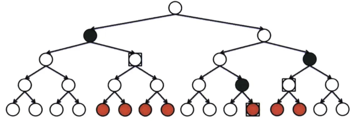
4-2 A sub-spanning-tree of depth 4 from Y in G. The red nodes are the missing
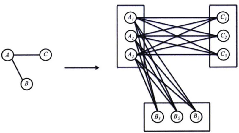
nodes. The green nodes are the potential malicious adversaries. The square-outlined nodes are the potential naive adversaries. . . . . 51 5-1 An example of the any-trust transformation when m = 3. . . . . 56
List of Tables
1.1 Performance of different protocols.
f
is the percentage of adversarial users am ong the population. . . . . 15Chapter 1
Introduction
All-to-all communication [26] is a popular topic in parallel computation. It is the general-ization of one-to-all broadcast in which all n nodes simultaneously initiate a broadcast. It is further classified into two categories, all-to-all broadcast and all-to-all exchange. In all-to-all broadcast, every node sends the same message and in all-to-all exchange, every node sends a distinct message. This problem commonly arises in parallel computation [13,19,22], where each node represents a processor and the algorithm's speed and message's size are analyzed. However, the use of all-to-all communication is not limited to parallel computation. Many large-scale distributed systems, especially voting and consensus protocols [10, 23, 27, 33], require all users to exchange authenticated messages with each others subject to adversarial attacks. Typically, to achieve an all-to-all broadcast, we either let each user broadcasts their messages individually, or elect a leader who gathers and broadcasts for all the n users. In the first solution, a user receives n messages and n signatures, which is undesirable for large-scale distributed systems that contain millions or billions of users. In the second solution, we leave everything to the leader. This minimizes the overall communication traffic in the network but inflicts a huge workload on the leader. It is also vulnerable to adversarial attacks because the leader's identity is generally publicly known and the leader can be easily corrupted.
Our objective is to let an honest user receive from almost all other honest users, while keeping the amount of network communication low and with low variance. A special
as-sumption in our protocol is that the users' messages have a constant number of bits. A user needs to receive at least n times the message size bits. This leaves little improvement if the message size is too large. We thus assume that the signatures take up most of the communication cost. We use aggregate signatures to construct a new all-to-all protocol, where (1 - Ej) fraction of the honest users are guaranteed to receive messages from at least (1 - E2) fraction of the honest population within E(log n) rounds. Here, El and e2 are two
small constant parameters that can be changed at will. Our protocol also upper bounds the number of bits each user receives by
E
(n log log2 n), which is a huge improvement from the conventional n times the signature size. Besides the all-to-all protocol, we also provide new results regarding random graphs and regular graphs. These results are used in our protocol to prove its efficiency. Further, they are interesting by themselves and have independent theoretic value.Let us formalize the problem mathematically. Suppose we have n users in the network and a constant
f fraction of them are adversarial. Each user 9 has a distinct short message
my of constant bit size. An honest user aims to gather all (or (1 - E) for a small E) ofthe honest users' messages. In our model, honest users always follow the protocol correctly, while a malicious user may deviate arbitrarily from the prescribed protocol. When new users register into the system, the adversary can corrupt them arbitrarily as long as the fraction of corrupted user does not reach the upper-bound
f.
However, the adversary cannot corrupt honest users or interfere in any way with the communication between honest users. In our model, an honest user will forever stay honest. Finally, we assume that the adversary is polynomially bounded in computational power. It cannot forge the digital signatures of honest users, except with negligible probability.1.1
Related Work
Almost-everywhere Byzantine agreement protocol: We adopt the "almost-everywhere"
concept [14] in our protocol. We do not require every user to receive from every other users, but instead aim to make sure that a large fraction of honest users receive almost
everyone's messages. This concept is frequently used in the design of Byzantine agree-ment protocols. Dwork et al. [14] first proposed an "almost-everywhere" Byzantine agreement protocol that works in networks of bounded degree. However, their proto-col only tolerates e(n/ log n) failures where n is the number of nodes in the network. This was later relaxed to
E
(n)
but the network degree has to be polynomial in n [35]. In [11], the network degree is relaxed to poly-logarithmic, making it more practical. Another related work [24] provides a poly-logarithmic time algorithm that agrees on a small representative committee based on the "almost-everywhere" BFT protocol. It uses O(n3/2) total bits and succeeds with high probability. Unlike these previous work, we do not require users to reach consensus. Our objective is to let honest users receive from almost all other honest users. The all-to-all message exchange is a key process in most BFT protocols, but it does not imply consensus directly.Random graph theory: The classic random graph model was proposed by Erd6s and
Renyi [15], where each edge in a random graph G(n, p) is independently chosen with probability p for some p > 0. In such random graphs, nodes all have the same expected degree np. Soon after, various random graph models were proposed to model more diverse degree distributions in applications [2-4, 25]. In this paper, however, we will focus on the initial Erd6s-Renyi model [15]. In particular, we care about the size of the giant component and the graph's diameter under the Erd6s-Renyi model.
The size of the giant component in a random graph where p = c/n for c near 1 is in fact a well studied problem. When c < 1, the size of the giant component is approximately
E(logn). When c = 1, the size of the giant component is asymptotically
E(n
2/3). And when c > 1, the size of the giant component is 6(n), with the second largest component around E(logn) (see [16] and [21]). When c > 1, we can also determine the expected size of the giant component as Een + o(n), where Ec is the solution to E + e-C, = 1 [5,32]. This result can be generalized to most of the other random graph models [31].giant component. The current state of the art is from Riordan and Wormald [34]. They show that in a random graph G(n, c/n) if c > 1 and c' < 1 such that cec'= cec,
then
login 2logri.
diam(G(n, c/n)) = logc + l + O(1) (1.1)
log C log 1/C"
holds with high probability. When c is large enough, even the O(1) term can be removed, showing that diam(G(n, c/n)) is almost exactly loga n - 2 logc, n. However, in all of the above works, a probability distribution is considered "high probability" if it goes to 1 as n -÷ oc. In most works, failure probability is inverse-polynomial or even inverse-polylogarithmic, which is not strong enough to apply in security applica-tions. In this paper, we will provide some general results that have negligible failure probability.
Distributed computation via all-to-all communication: Another related area of
re-search is to utilize a distributed network to calculate a function
f(-)
when nodes have only partial inputs and limited connectivity [17]. Depending onf(-),
the algorithms can be vastly different. Our research can be considered as a generalized case of this problem. If users successfully perform an all-to-all broadcast round, then all users would have the complete inputs. They can then compute the functionf(-)
indepen-dently.1.2
Overview
In this paper, we provide two protocols for the all-to-all broadcast problem. The first one is the random query protocol. It requires a gossip network where each pair of users shares a communication channel. Users randomly query others for messages until all messages are collected. The random query protocol has a parameter d that measures how many users one should query in each round. Different choices of d can result in different round numbers and communication costs, the details of which can be seen in table 1.1. Our second protocol is the fixed topology protocol. Instead of querying random users in each round, we query a
fixed set of users every round. Users don't need to establish new connections every round and can receive almost all of messages even with limited connectivity.
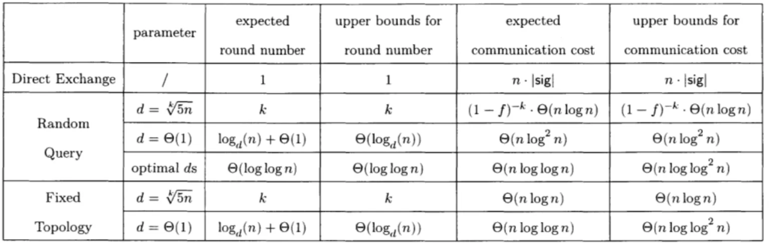
Table 1.1: Performance of the population.
different protocols.
f is the percentage of adversarial users among
In table 1.1, we listed the performance of our protocol under different parameters. The tpper bounds in table 1.1 are probability upper bounds, meaning that the round numbers and the communication costs are less than them with overwhelming probability. It is hard to characterize our work in just one table. For example, the constant overheads of the big
E
depends on a lot of parameters, so it is hard to write them out explicitly. But almost of our constant overheads are small constant less than 5. In general, the random query protocol offers the least communication cost. The fixed topology protocol, on the other hand, is easier to set up and offers a stronger security guarantee. We will revisit where exactly should each protocol be applied after we have introduced the protocols in detail.
expected upper bounds for expected upper bounds for
parameter
round number round number communication cost communication cost
Direct Exchange / 1 1 n -Isigl n -sigl
d = /5-n k k (1 - f)k -E(n log n) (1 - f)-; -(nlogn) Random
Query d = E(1) log,(n) + E(1) E(logd(n)) e(n log2n) O(n log2 n)
optimal ds E(log log n) E(log log n) E(n log log n) E)(n log log2 n)
Fixed d = k5n k k E(n log n) 9(n log n)
Chapter 2
Preliminaries
In this section, we introduce the fundamental tools needed to construct and understand our protocol, including aggregate signatures and verifiable random functions. We will also go over the high level ideas of our protocol.
2.1
Aggregate Signature
Suppose Alice has received messages and signatures from multiple users, is it possible for her to send them to another user without sending the messages and signatures directly? In other words, Alice need to convince Bob that the messages are indeed what she received without sending the signatures all over again. If this is possible, then users can recursively query for messages while only demanding small proofs/signatures. The tool that we use for this objective is the aggregate signature scheme.
Given n signatures on n distinct messages from n distinct users, an aggregate signature scheme allows one to aggregate all these signatures into a single signature. This single signature (and all n original messages) will convince any verifier that the n users signed the
n original messages. The idea of aggregate signatures dates back to an open problem by
Micali and Rivest [29]: Can intermediate links in the chain be cut out given a certificate chain and some special signatures? An aggregate signature partly solves this problem by allowing
for the compression of certificate chains. The first aggregate signature was introduced in
[7],
where an efficient aggregate signature is constructed from a short signature scheme based on bilinear maps [9]. Later, other variations like sequential aggregate signatures [28] and synchronized aggregate signatures [1, 20] were proposed. In our case, the aggregate signature scheme in [7] is sufficient. More details about aggregate signatures can be found in a good survey by Boneh et al. [8]. We present the detailed definition of the aggregate signature scheme below.Definition 2.1.1. A signature scheme (Gen, Sgn, Vf, agSgn, agVf) is an aggregate signature
scheme where
. Key Generation: Gen(1) returns a private signing key sk for the user and a public verification key pk for the verifier.
. Sign and Verification: Given a message m and the private key sk, a user signs by calling the Sgn function sig = Sgn(m, sk) such that
- Correctness: Vf(Sgn(m, sk), m, pk) = 1.
- Secure: for any polynomial adversary A that can access Sgn as an oracle, Pr(m',sig')--A(.) [Vf(sig 1] = negl(n).
. Signature aggregation and agg-verification: n signatures from users
{(mi,
sig (m.))}can be aggregate into a new short signature using the agSgn function sig"gg = agSgn (sig, (mi), - ,si
such that
- Effectiveness: sig,,9 is approximately the same size as sig,(mi) for any i. - Correctness: agVf(sig,,g, mi, - , mn, pk,, - , pk,) = 1.
- Secure: for any polynomial adversary A with oracle access to
{Sgn
2}j,
Pr [agVf(sig gg, {m }, {pki}) = 1] = negl(n).
* Aggregation of aggregate signatures: the agSgn function is not only applicable to original signatures, but also to aggregate signatures.
Given an aggregate signature sig,, - agSgn (sig(m1), -- ,- sig, m)), we say that user 1 to
n are components of the new signature siggg
By Definition 2.1.1, in order to verify a aggregate signature, we need to have the original
messages and each component's identity. Therefore, a complete aggregate signature should contain (1) the aggregate signature sigagg, (2) a message set M and (3) an array V which stores the set of components. For each of sig gg 's component, V stores its user name and the
number of times this component appears in sig (the count number).
We can use either a sparse array or a dense array to store V. A sparse array stores the user name and the count number for each component in sig; while a dense array stores the count number for all users, whether or not the user is a component of sig. Suppose each count number takes up c bits. For a aggregate signature with m components, the sparse array requires m - (log2 n + c) bits, while the dense array requires c - n bits. Therefore, a
sparse array should be used if and only if
c-n c-n
m- (logn + c) <cin ->m< .
n m
log n+ c log n
Since we assume the message size to be constant, the message array requires only 0(m) bits, which is negligible compared to the count array's size. And overall, the communication cost is mainly decided by the count array's cost. In the rest of this paper, we will focus on upper bounding the count array's size.
In most of the paper, we will use sparse or dense arrays to represent count arrays. How-ever, in certain scenarios, these two data structures are not enough to provide a sound solution. In these cases, we will introduce other complex structures that are designed specif-ically for the corresponding scenarios.
2.2 Verifiable Random Function
In our protocol, we frequently rely on a "pseudorandom oracle" to provide randomness and thus strong unpredictability. However, a pseudorandom oracle is not verifiable. Without knowledge of the seed, upon receiving the value of a pseudorandom oracle, one cannot distinguish it from an independently selected random string of the proper length. The adversary may thus declare any value it sees fit as the random result without fear of being detected. This is why, instead of a pseudorandom oracle, we want to use a pseudorandom function that is verifiable, namely, a verifiable random function (VRF).
The concept of verifiable random functions was initially proposed by Micali etc. in
[30]. Their idea is to combine unpredictability and verifiability by extending the
Goldreich-Goldwasser-Micali construction of pseudorandom functions [18], creating a random number generator that can be efficiently verified. A simpler and more efficient construction was later proposed by Dodis and Yampolskiy [12]. Their proofs of security are based on a decisional bilinear Diffie-Hellman inversion assumption. And for small message spaces, which is our case, their VRF's proofs and keys both achieve constant size. We provide the detailed definition of verifiable random functions as shown below.
Definition 2.2.1. Let G, F and V be polynomial algorithms where
* G (the function generator) is probabilistic. It receives as input a unary string (the security parameter) and outputs two binary strings (the public key pk and secret key
sk).
. F = (F1, F2) (the function evaluator) is deterministic. It receives the secret key sk and
a seed x as input, and outputs the value v = F1(sk, x) and the proof p = F2(sk, x).
. V (the function verifier) is probabilistic. It receives pk, x, v, and p as input, and
outputs either 0 or 1.
We say that (G, F, V) is a verifiable random function if
0 Unique Provability: For all pk, x, v
0, vi, po, p, such that vo * v1,
Vi = 0, 1, Pr[V(pk, x, Vi, pii) = 1] is negligible.
Residual Pseudorandomness: : Let T = (TE, TG) be any pair of algorithms such
that TE and TG run for a total of at most s(k) steps when their first input has length k. Then, the probability that T succeeds in the following experiment is at most 1/s(k):
- Run G(1k) to obtain pk and sk;
- Run TsF(sk-)(Ik, pk) to obtain (X, state);
- Choose r +- {0, 1}. If r = 0, let v = F,(sk, x). If r = 1, choose v randomly;
- Run T F(sk,)(lk, v, state) to obtain guess;
- T succeeds iff guess = r and x was not queried before on the F(sk, -) oracle.
In short, a verifiable random function allows the user to provide verifiable yet unpre-dictable randomness. However, in order to be verified, one must send the proof to others which adds to the communication cost. Thus, VRF should be used only in scenarios where strong security properties are needed.
2.3
A General Algorithm
Now that we have the tools we need, we can provide the skeleton of our algorithms. The key ideas are simple. The protocol is synchronous and consists of multiple rounds. In each round r, a user Y selects a set of users S, queries users in S, for the signatures they have and aggregates the feedback. This is repeated for number of rounds such that the user is guaranteed to receive (1 - ,) of the honest signatures with high probability. Our goal is to design {S}gr such that the communication cost is minimized.
Algorithm 1 General algorithm for a user S Input:
User Y's message mj. Sets S', ., S.
The aggregate signature scheme (Gen, Sgn, Vf, agSgn, agVf). Algorithm:
1: (sk, pk) +- Gen(1k).
2: sig +- Sgn(sk, mj).
3: Create a message array M9 and set M[] <-i my. 4: for i = 1 to r do
5: For each X
C
Sy, query X for the message array Mx and the aggregate signature*i-i sig"
6: Authenticate the received messages using agVf and discard any message that fails. 7: sig, <- agSgn({(sigxi 1, My[X]) I X E Sg U {S}).
8: M- <- UJCES"u{1J} MX'
Chapter 3
All-to-all protocol with simple
random queries
We start by setting all the S' in Algorithm 1 as a random set of size d. In each round, users randomly select a set of d users and query these users for their aggregate signatures. This is repeated until the user gathers 1 - El of the signatures. It is important that the random
sets are selected via verifiable random functions. Upon receiving a query, a user can verify that the query is indeed randomly generated. We say that a user 7 has received user X if and only if 3's aggregate signature contains X. Specifically, X is received by J in the ith
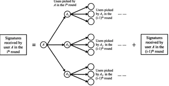
round iff X is a component of sigi. In Figure 3-1, we provide an illustrative understanding for the set of users received by Y in the ith round.
In the first round, a user 7 queries d distinct neighbors and receives exactly d
+
1 signatures (d new signatures plus 7's original signature). In the second round, Y receives d new aggregate signatures, each with (d+
1) components. Due to possible collisions betweenthe aggregate signatures, the number of signatures received in the second round is generally smaller than (d + 1)2. 7 receives (1) the d + 1 distinct users queried in the second round (including himself) and (2) the d(d + 1) users randomly queried by users in (1) in the first round. This reduces our problem to the classic problem of "how many distinct balls can be picked after some sample-with-repetition trials". Let us make this formal. We denote S(i)
Users picked by A in the Ph round A, Signatures received by A 2 user A in the itj round A3 Users picked by A, in the ... ... (i-I)h round Users picked byA2inthe +.
(i- I))1 round
Users picked
by A3 inthe (i-1)h round
Figure 3-1: Signatures received by a user in the ith round.
as the cardinality of the set achieved by independent and identically sampling i times on the users
{1,
... , n}. In other words, S(i) is a variable that denotes the number of distinctelements we get after i i.i.d. samplings on
{1,
, n}. It is clear that 7 receives at leastS((d + 1)2) signatures in the second round.
We can characterize the above idea and generalize it to the ith round as in Figure 3-2. From Figure 3-2, we know that in the ith round, Y receives (1) the d + 1 distinct users 9 queried in the it
h round and (2) the users received by users in (1) in the (i - 1)th round. Our objective is to lower bound the number of users received in the rth round where r is the number of rounds in Algorithm 1. We consider Figure 3-2 where i is set as r and denote R' as the set of users in the jth layer in Figure 3-2's tree. An immediate observation is that
{} = RO C R' C ... C Rr. Similar to our analysis in the previous paragraph, we can show
that JRJ| > S((d + 1)|R'-1|) holds for all 1 < i <r.
3.1
Lower bound for Sample-with-repetition
We have shown that IR'I is closely related with the S(-) function. So in this subsection, we analyze the process of select with repetition and try to lower bound S(i) for any 1 < i < n.
Signatures received by userA in the
Sigatur
received by - The last layer of user A in the
i*h rund
Figure 3-2: New representation of signatures received by a user in the ith round.
In Lemma 3.1.1, we lower bound S(i) for different possibilities of i's values.
Lemma 3.1.1. We provide two lower bounds for S(i) based on whether i > V/ni. " If i < /,0.6, Pr[S(i) < i - Vi] < (e. il./2n)v.
" If i ;> Vn0, Pr[S(i) < i - 2i2/n] = negl(n).
Proof. We consider i sample-with-repetition processes on
{1,
-, n} and denote the jthsam-ple as aj. We also denote Aj as the event that aj collides with former samsam-ples, Aj equals 0 if a3 0 {a,, ... , aj-1
}
and 1 otherwise. Instead of computing S(i) directly, we can computethe number of collisions between
{al,
., a}
which equals i - S(i).jS(i) = E A j= E A j=1 j=1 Pr j=1 j=1 j -1 n ~ . 2 ) (3.1) IUsers
picked Users picked
byA, in the the i* A, (i-1)*round -round A, A, Users picked A by A2 in the A2 (i-ly round ----Users picked A by Aj in the A3(Wi-hround ---A3 Users picked A by A in the A ~(i- Ithround 1 -...
Using Chebyshev's Theorem, we have
= Pr [ZA >
j=1
= Pr e E Ai > et es I~> < E[et- 1 ets j] (3.2)
In equation 3.1, Pr[aj E {a1, -- , aj_1}] ; (j - 1)/n holds regardless of the set {a,.-- , a 1}.
Therefore, for any s E [0, i] and any t > 0, Ai] =E IjetAi J (1 + j=1 j=1 j -1 ____I. ), - -2 S- 1. et . ]I .x( e e et).- (3.3) n ~j=1 n2
Combining equation 3.2 and 3.3, we get that for any t > 0,
Pr[S(i) < i - s] < exp( i2 et - ts). 2n
The exponential term (i2/2n) - et - ts reaches its minimum when t = ln(2ns/i2). Thus
long as s > i2/(2n), we can take t = ln(2ns/i2) in equation 3.4 and achieves Pr [S(i) < i - s] < exp(-s(ln( j2 ) - 1)).
Finally, we set s in equation 3.5 to be the desirable value to complete our proof: . If i < n0 6, we set s= Vz- and t
= ln(2n/i- 5). Thus,
Pr[S(i) <i -
V%]
< (e il-5/2n)v'.- If i > n0 .6, we set s = 2i2
/n and t =In 4. Thus,
Pr[S(i) < i - 2i2/n] < exp(-(i2//n)) = negl(n).
In all the cases above, we set t to be larger than 0 so equation 3.5 can be safely applied. We then give another lemma which shows that S(i) becomes very close to n as i grows.
.4) as 3.5) Pr [S(i) -8] E [etZ= E
Lemma 3.1.2. For any constant E e (0,1), there exists a constant c, such that S(cen) >
(1 - E)n with overwhelming probability.
Proof. We will prove using induction that S(k - 0.11n)
>
(1 - 0.92k)n for any constantk > 1. By Lemma 3.1.1, S(0.11n) > 0.08n with overwhelming probability. Thus, the
statement holds when k = 1. Assume the statement holds for a constant k > 1, we will try
to prove the correctness of the statement for k + 1.
Given (k + 1) - 0.11n samples, we consider the first k - 0.11n samples. By assumption, the first k - 0.1In samples contain at least (1 - 0.92k)n distinct elements with overwhelming
probability. Thus, there exists a subset N from the first k - 0.11n samples such that INI =
(1 - 0.92k)n. We denote the last 0.11n samples as set M and claim that the following two
events happen with overwhelming probability.
. At least 0.1(rn - IN1) samples among M are not in N.
Proof idea: the probability of a new sample not being in N is (n - INI)/n. This is independent across all the new samples. We can then show using the Chernoff bound
that this event happens with overwhelming probability.
. IM/N > 0.08(n - NI), i.e., new samples cover at least 8% of [n]i/N.
Proof idea: we have already shown that at least 0.1(n -I N) of the new samples is in
[n]/N. By Lemma 3.1.1, these 0.1(n- NI) new samples contain at least 0.08(n- NI)
distinct elements with probability negl(n - INI) = negl(n).
Therefore, S((k+1) .O.1ln) > |M/NI+NI = 0.08-0.92kn+(1- 0.9 2k) -n = (1-0.92k+1) .n with overwhelming probability. This completes our proof of induction. l
Lemma 3.1.2 implies that S(55 x 0.1ln) e S(6n) > (1 - 0.925 5)n ? 0.99n with
overwhelm-ing probability. However, much of the inequalities in Lemma 3.1.2 are relaxed. Through
experiments, we find that S(4.5n) exceeds 0.99n with overwhelming probability. We provide
the experimental result below and claim without proof that one cannot deviate far from the
Claim 3.1.3. When i = 8(n), Pr[S(i) < (1 - E)E[S(i)]]= negl(E2n)
for any constant e.
The plot of (i, E[S(i)]) is shown in Figure 3-3.
0.8 C 0.6 0.2 D-0 1 2 3 4 5 In
Figure 3-3: Experimental simulation of E[S(i)] against i.
3.2
Correctness proof when all users are honest
Given Lemma 3.1.1 and 3.1.2, we are ready to analyze our protocol. In this section, we will
set the E, to 0.01 so that we can make our arguments more concrete. A user is considered
successful if and only if it has received 0.99n of the signatures after our protocol. To start
with, we first analyze the protocol under the assumption that all users are honest. We will
then provide a way to modify our analysis to include adversarial attack. We start by showing
that for appropriate choices of the degree d, Algorithm 1 terminates in constant rounds and
the number of bits each user receives is bounded by 5n log n.
Theorem 3.2.1. If d = V53n - 1, where k is a constant number greater than or equal to
2, then Algorithm 1 terminates within k rounds and the number of bits each user receives is bounded by 5n log n.
Proof. We first show that jRkj > 0.99n with overwhelming probability, which implies that
Algorithm 1 terminates within k rounds. For convenience, we define the function 6(i) as
shown below:
1 /(%- i < 1n
By the second bound of Lemma 3.1.1, S(i) > (1 - 6(i))i with overwhelming probability.
Denote A2 as the event that R'I > (1 - 6((d
+
1) - IR-yIl)) - (d + 1) R'-1 . We have alreadyshown that IR I > S((d + 1) R- -1), therefore by Lemma 3.1.1, Pr[A] = 1 - negl(n). If all of the events
{Ai}r_-
1 hold, thenk-1 IR kJ > S ((d + 1)k. -J (1 -
6((d
+ 1) R-I))) i=1 k/2-1 k-1 > S 5n - 11 (1 - d-'/2 . _I i=1 i=k/2 k/2-1 k-1 >S S5n (- ( E - d-i/2 _ d i=1 i=k/2 > S(5n - (1 - 4d-o 5)) > S(4.5n),which is larger than 0.99n with overwhelming probability by Lemma 3.1.2. Using union bound, we have
k-1 k-1
Pr[A AJ] > 1 - Pr[--,A] > 1 - (k - 1)negl(n),
i=i i=i
which is still negligible. In conclusion, all the users receive 99% of the signatures at round k with overwhelming probability. It remains to calculate the total number of bits a user receives. Signatures received by users will have at most dk-1 = 5n/d components, which is significantly less than the transition
E
(n/
log n). Therefore, we should always use sparse arrays to record aggregate signatures. In the ith round, a user receives d aggregate signatures each with (d+ 1)i- components, which needs d(d+ 1)i- log n bits. Summing all the roundsup, the total number of bits received by a user is 5n log n. D
In conclusion, if we set d = V5Y, then the protocol requires k rounds. The communication
cost for each user is 5n log n and the failure probability is negligible. We will now analyze the performance of Algorithm 1 when d is of smaller value and even just a constant. When d is constant, we cannot bound JR'J with overwhelming probability. Lemma 3.1.1 does not provide an overwhelming probability bound for S(i) when i is small. To analyze the protocol
when d = Q(1), we need new tools to analyze and approximate IRI.
Lemma 3.2.2. If IR| = cn, where c = E(1), then E[IR'J 1 I R'l = cn] ~ cn+(l-c)E[S(d. cn)]. Moreover, given
|R|=
cn, the probability that IR'+| deviates a constant factor fromE[|R'1| | |R'| I= cn] is negligible.
Proof. The proof is similar to the proof of Lemma 3.1.2. We know that R"' is made up of R'
and the dIR'I new samples. Among the dIR'I new samples, c -dIRgI of them are expected to be in R'. Therefore, the expected size of R7' should be IR I
+(1-
c)E[S(d -cn)]. And using the Chernoff bound, we can show that R' does not deviate far from its expectation. IIWe can now state our main result for this subsection in Theorem 3.2.3.
Theorem 3.2.3. When d = E(1), Algorithm 1 terminates within logd+1(n) rounds with
1-E(n-(d+l)) probability. The number of bits each user receives is bounded by E(n log log n).
Proof. We first show that there exists an r = logd+1(n)
+
0(1) such that R > 0.99n with 1 - 0(n-(d+l)) probability. This upper bounds the round number. Before we start, we provide some new notation. We define a new function Fd(x) = x+(1-x/n)E[S(d-r)], which corresponds to the expectation of R' in Lemma 3.2.2. For convenience, we also define a new variable r, = _log+ 1(0.1n)J
that will be used later. Our proof consists of two parts. Firstly, we show that IR'I is lower bounded by 0.08(1 - 2d')n with 1 - 0(n-d-1) probability. Secondly, we show that ifIRg|
= 6(n), then Algorithm 1 requires at most another 6(1)rounds to terminate.
In the first part, we aim to prove that
IRy
> 0.08(1-2d1 )n with 1- (e(d + 1)3/2n)d+1probability. We have already shown that
IR'I
> S((d+
1)1R'y'I). Thus, we can use Lemma3.1.1 to lower bound S((d + 1) IR'T1) by (1 - 6((d + 1)IR'-'I)) - (d + 1)IR'71I, where the 6(-) function is defined in the proof of Theorem 3.2.1. This in turn lower bounds JR'l. Let us denote Ai as the event that
Suppose the event Ai holds for all 1 < i
<
rl, then one can easily show by induction that IR'l > d'. Also, by its definition, IR'l must also be upper bounded by (d + 1)'. Thus,A
1 Ai implies that rj-1 > (d + 1)yj - (I - 6((d + 1) - I R'j)) 0.6 logd+1 n r > (d + 1)r1- ( 6((d + 1) I R'j)) -i=0.61 0.6 log,+1 1 r-1 > (d +1)r -J
(1- ) -17
i=1 i+ I i=0.6 log d+ I n+1
0.6 log,,+1 n 11
> (d + 1)Y1 (I - E di+ Y
i=1 N/d-+1 i=0.6 log,+ n+1
1 1 > (d+1yi ( - -0.2(1+ 1) d- 0d d + 1 > 0.8(l - 2d-1) - (d + 1)r1 > 0.08 - (I - 2d-')n. + 1) - IR'l)) 1 (1 -1( :)gd+l n+1 -2(d + 1)i+1 i+ 2(d+1)' n
Using Lemma 3.1.1, we can lower bound the probability of
A
1 A using union bound,rj-1 rj-1
Pr[{R| > 0.08(1 - 2d-1 )n] > Pr[
A
Ai] > 1 - Pr[-,Ai] > 1 - (e(d + 1)3/2n)d+lThis completes our proof for the first part.
In the second part, we aim to show that there exists a constant r2 such that F2 (|R, ) >
0.99n. We will show that for any d, there exists a constant Cd > 1 such that if s < 0.99n then Fd(s) > CdS. Therefore, the above claim obviously holds. Although Fd(.) is hard to express explicitly, we can use the fact that Fd(-) is a deterministic function and simulate it with programs. Simulation reveals that when d = 2, r2 = 5; when d = 3, r2 = 4; when
d = 4,5,6, r2 = 3; when d
>
7, r2 <2. Recall that Fd(x) is the expected value of IR+ 11 when IR I = x. Fd 2(IR'1g) > 0.99n implies that E[ R1+r2|] is expected to reach 0.99n. By Lemma 3.2.2, we know that the actual IR7 +r2 cannot deviate far from from its expectation.Combining this with the first result, we have that our protocol terminates at round r,
+
r2with 1 - (e. (d + 1)3/2n)d+1 probability.
It remains to calculate the number of bits a user received. Since d = E(1), a user's
aggregate signatures' component size can range from 1 to 0(n). Therefore, we should use a sparse array in early rounds and then switch to a dense array in later rounds. The transition happens at the round where signatures have 8(n/ log n) components, i.e., at round rt s.t. (d + 1)rt = (n/log n). Thus, the total number of bits a user received is
10gd+1 n-109d+1 log n 109d+1 (n)+ E)(1)
log n d. (d + 1) + E(n) = dn + E(n) -log log n. (3.6)
=9dog +1 n~-10 ( 1 logn
This ends our proof. D
The performance shown above is theoretically better than the results in subsection 3.2. The constant factor before the communication cost depends on r2 (the number of rounds in
step 2), which in turn depends on d. In practice, the count number rarely exceeds 30, thus we can use 5 bits to record a count number. In conclusion, when d = )(1), the protocol
requires logd+1(5n)+ (1) rounds and fails with E)(1/nd+l) probability. The communication cost of each user is E( (n log log n). Compared to when d = VSn, we decrease the number of
bits users receive while sacrificing number of rounds and failure probability,
3.3
Optimal degree combination
In general, the degree d should be chosen such that 3k E Z, Fj(1) = 0.99n. This means that a user receives exactly 99% of the signatures at round k. To illustrate why such choices of d are desirable, let us consider the cases when d = 0.9v/5n, d = S5i and d = 2V 5
correspondingly. When d = v"5, F2(1) e S(5n) m 0.99n. The algorithm terminates at round 2 and each user receives 5n log n bits of message. When d = 2 "5H, the algorithm still takes two rounds to complete. But users now receive d2 log r = 20n log n bits of message,
algo-rithm takes three rounds to complete. Each user receives
E(n'
5 log n) bits, which is veryinefficient. From the above examples, we can get an intuition as to why we should set d such that Fj (1) = 0.99n.
Another solution, which allows us to select the degree d at will, is to use d for the first r - 1 rounds but choose a new degree d' at the last round. Here, r is used to denote the total number of rounds. d' should be chosen such that Fd/
(IR'-|)
~~ 0.99n. Let us reconsider the cases where d = 2 5n and 0.9 5m. When d = 2V5'n, the user should select 2v S neighbors in the first round but only 0.5 5n neighbors in the second round. The algorithm still finishes in two rounds, but each user only receives 5n log n bits of message. When d = 0.9v5n, the user should select 0.9 5m neighbors in the first two rounds and 2 neighbors in the third round. Each user receives 8n log n bits, which is much better than the originalE(n
.5 log n).We have seen that changing d's value in the last round improves performance. The questions naturally arises as to whether changing the value of d at other rounds improves performance as well. Specifically, if we are allowed to use a different degree value di at each round i, then what is the optimal degree combination
{di}?
In section 3.2, we discuss two choices of d. When using large d, we can apply the Chernoff bound and get negligible failure probability. But using small d allows us to use the dense array to its full potential, thus having aE(n
log log n) communication cost. So if we use large d at first and then switch to small d later, is it possible to have a E(nlog
log n) communication cost while having a negligible failure probability?The answer is yes! In fact, we can even show mathematically that using large d's followed
by small d's is the "optimal" solution. We start by considering a related problem. If every
user has i signatures at the moment, what is the optimal degree choice for them in the next round? Let us denote G(i) as the expected number of bits a user need to further receive when it has i signatures. We can approximate G(i) greedily as:
G(i) ~ min[d . Cost(i) + G(Fd(i))],
d
i, we can calculate G(i) from i = 0.99n to i = 1 recursively. Given G(i), we can easily compute the optimal degree combination
{dj}
1 as in Algorithm 2. In Algorithm 2, D(i)Algorithm 2 Compute the optimal degree combination. 1: Set G(x) +- 0 for all x > 0.99n;
2: for i = 0.99n to 1 do
3: Set D(i) <- argmind[d - Cost(i) + G(Fd(i))];
4: Set G(i) <- D(i) - Cost(i) + G(FD(i)
5: end for 6: s +- 1, i <- 1; 7: while s < 0.99n do 8: d4 D(s); 9: s -Fdi(s); 10: i i + 1; 11: end while
12: Return the combination
{di};
is the degree a user should choose when it has i signatures. The result of Algorithm 2 is that di = d2 =
E
(n/
log n) and d3 = -= d 1. Detailed observations show that d, and d2 are approximately the square root of the transition (between the sparse-array anddense-array). This matches the intuitions we mentioned before:
. Suppose it takes r, rounds to reach the transition, i.e. F21 (1) = transition. Then,
during the sparse-array period, a user receives approximately (d + 1)'1 - log n bits, which is minimized by setting d, and d2 as the square root of the transition.
. After we reach the transition, we should set d to be as small as possible to exploit the advantages of dense-array representation. The reason why d = 6(1) outperforms
d = /5-n is because it uses dense-array at later rounds. Dense-array provides a
significant improvement over the sparse-array when a signature's component number is
9(n).
The intuition is similar here.This gives us a scheme which has 9 (log log n) rounds and negligible failure probability. The communication cost of each user is 8(n log log n). The optimal degree combination inherits the advantages of both d = E(1) and d = k/5n. It has near-optimal performance in terms of latency, failure probability and communication cost.
3.4 Proof of correctness and security under an
adver-sary setting
In this subsection, we will analyze adversarial attacks and describe how we modify our pro-tocol to prevent them. The adversary's objective is to (1) stop honest users from receiving other honest users' signatures and (2) increase the number of bits an honest user receives. Although a malicious user may perform arbitrarily, it should not take actions that immedi-ately reveal its maliciousness. In fact, all malicious actions that do not reveal their identities can be divided into two categories.
. Hide signatures from honest users. A malicious user Eve may receives signatures from Alice, Bob and Carl, yet deliberately ignores Alice's signature so that Alice appears disconnected from the network.
. Merge other malicious users' signatures into messages. Only honest signatures matters to honest users. Therefore, a malicious user can merge other malicious users' signa-tures into its aggregate signasigna-tures. This increases the number of components/bits of the aggregate signatures, while keeping the signatures valid. However, the signature sizes (number of components in the aggregate signature) must not exceed the protocol's assumed theoretical upper bound. Otherwise, the malicious user would be easily rec-ognized and its action becomes equivalent to a DDOS attack, which is not considered in this paper.
We now consider the effect the adversary has on our protocol. Suppose
f
percentage of the population are adversarial, one immediate solution to counter the adversary is to increase the degree from d to d(1 -f)-
1. A user will still be connected to d(1 - f)-1(1 -f)
= d honest users in expectation. The honest subgraph remains well-connected and 99% of the honest signatures will be received at round r. However, by increasing the degree, the size of the signatures/messages increases correspondingly.the number of components. Since we have increased the degree from d to d(1
-the number of components grows from d' to d(1 -
f)i
in the ith round. Thus, when the adversary exists, the message size is scaled by a (1 - f)-- factor in the ith round.If the signatures are recorded using the dense-array, the message size is approximately
n times the log of the count number. Here, the count number means the maximum
number of times a component appears in the signature. The count number grows from
E(d
/n)
to 0(d2 - (1 - f)-/n). Thus, in the ith round, the message size is increasedby
log(E(di(1 - f)-i/n)) - log(O(di/n))) n = log(E((1 - f)-i)) n =
e(in).
With the sparse-array representation, the increase is exponential with i. While with the dense-array representation, the increase is only linear with i. The intuition is that one should set d such that more dense-array representation is used in the protocol. We now compute the detailed communication cost increase for different choices of the degree d.
. When d = V5 for some constant k, we use the sparse-array throughout the entire algorithm. The algorithm has k rounds, thus the number of bits an honest user receives is increased by a (1 - f)-k = E(1) factor.
. When d = E(1), we use the sparse-array for (logd+1 n - log 1 log n) rounds, then
switch to the dense-array for (logd+1 logrn + E(1)) rounds. However, due to the in-crease of signatures' sizes, we will reach the transition much earlier, i.e., at round
logd_(1 _ (n/ log n). So we will be using the sparse-array and dense-array for e(log n)
rounds each. Therefore, the number of bits an honest user receives is
(costs in sparse-array rounds) + (costs in dense-array rounds)
log ( _p 1 (n/ log n) i=8(log )
d (1E- )- 8(i -n) = E(n log2n).
. Finally, we consider the optimal degree combination in subsection 3.3. The optimal combination takes two rounds to reach the transition, then
e(log
log n) rounds to complete. Therefore, the number of bits an honest user receives is approximatelyE
(n log log2 n), which suffers only a small increase from the original E(n
log log n). We assume a static adversary in our model, i.e., the adversary cannot corrupt any user after the protocol begins. It is worth pointing out that the above analysis still holds even when facing a semi-dynamic adversary. A semi-dynamic adversary can corrupt any user at any time it wants, even after the protocol begins. However, the corruption takes a while to take effect. Specifically, if two users Y and K are honest when Y initiates a query request to X, then even if the adversary immediately tries to corrupt K, the corruption will not take effect until X finishes its reply. This means that Y always receives an honest reply from K. The model of semi-dynamic adversary is a very powerful one. The fact that a malicious user can both hide (signatures) and add (components) means that it can replace any signature that passes through it with a meaningless signature of arbitrary size. If we can restrict the adversary from adding arbitrary components, the communication cost might be even lower. Another issue with the Random Query Protocol is its extensive use of verifiable ran-domness. In each round, a user needs to select d random neighbors, which requires d log n verifiable random bits. This does not add much to the communication cost, but still creates inconvenience for the users.Chapter 4
Random Graphs and the Fixed
Topology Protocol
In this section, we propose a new protocol that addresses the two problems in Random Query Protocol. Instead of reselecting new random users in each round, we fixe a graph G = (V, E) and let users repetitively query their neighbors. Users still follow the general
algorithm (Algorithm 1) but the input S" is fixed as the neighbors of Y in G. And since users will be querying the same set in each round, the query process can be modified to increase efficiency. Specifically, when user J is queried in the ith round, it should reply sig /sig instead of sigh, because sig- was already replied to in the previous round. We describe the algorithm in pseudocode in Algorithm 3.
In Algorithm 3, we construct G as a random undirected graph where each edge exists with probability d/(n - 1). In expectation, each user has degree d and the number of edges E[|E|] is nd/2. It is worth pointing out that there are other possible constructions for G that offers useful properties. For example, we could construct G as a random d-regular graph so that each user queries exactly d neighbors in each round. Or we could construct G as a directed graph instead of an undirected one. We have tried several models; all of them give roughly the same performance. In fact, it can be proved that most of the constructions are equivalent. In this section, we will focus on the case where G is an undirected random
Algorithm 3 All-to-all broadcast algorithm for a user 7 under the weak adversary model Input:
The degree parameter d and security parameter E. The user's message m.
The aggregate signature scheme (Gen, Sgn, Vf, agSgn, agVf).
A randomly generated topology G = (V, E) where each edge exists with probability
d/(n - 1).
Algorithm:
1: (sky, pk,) - Gen (1k).
2: sig" +- Sgn(sky, my).
3: S_ +- 's set of neighbors in G.
4: Create a message array Mj and set Mj[] +- im.
5: For each of Y's neighbor X, create a special variable siggj, initialized as sig 0 6: while i <- 0; sig' contains less than (1 - E)n distinct signatures do
7: For each X Ce Sy, query X for the message array MX and the aggregate signature sig _ .
8: Authenticate the received messages using agVf and discard any message that fails.
9: sig' +- agSgn({(sigx, 1 , M1 [X])
I
X c S U {1}}).10: For each neighbor X, sigj_, = sig
/{sig
-', sig }.11: Mg +-- UXES-etpj Mx.
12: i +- i+1.
graph. Particularly, we will show that any user running Algorithm 3 terminates within a reasonable number of rounds and has small communication cost.
To analyze the performance of Algorithm 3, it helps to first consider the case where all users are honest. This gives us intuitions as to why Algorithm 3 works and the potential attacks the adversary may use. When all users are honest, we can prove Lemma 4.0.1.
Lemma 4.0.1. Define dist(g, X) as the distance between two users . and X in G, and D'
as the set of nodes exactly i nodes away from ., i.e., D' - { X I dist(Y, X) = i}, then * there exists no edge from D' to D' for any i' - i > 2.
" if all users follow Algorithm 3, then the set of users received by 7 in the ith round is R' = U1 D' . Moreover, if two users 7 and X are connected in G, then eventually -7
and X will receive each other's signatures.
Lemma 4.0.1 shows that any two connected users in G will receive each other's signature. We use the giant component to describe a graph's largest connected subgraph. Therefore, users in the giant component will be able to receive signatures from each others. And if the giant component's size exceeds (1 - E)n, then at least (1 - e)n of the users will receive
(1 - e)n signatures.
4.1
Connectivity and giant component in random graphs
The relationship between the size of the giant component and the degree d has been one of most the most studied areas in random graphs. It has been shown in multiple papers
[6,15,16, 21] that the expected size of the giant component becomes exponentially close to
n as the degree d grows.
Theorem 4.1.1. For a random graph with degree d, its expected giant component size is sn where s = 1 - e-s
Like in Theorem 4.1.1, most previous work are concerned with the expected size of the giant component or be simply satisfied with inverse-polynomial failure probabilities. But in

![Figure 3-3: Experimental simulation of E[S(i)] against i.](https://thumb-eu.123doks.com/thumbv2/123doknet/13930209.450619/29.917.270.605.187.368/figure-experimental-simulation-of-e-s-i-against.webp)