An analysis of finite parameter learning in linguistic spaces

(1)

An Analysis of Finite Parameter Learning in

Linguistic Spaces

by

Karen Thompson Kohl

Submitted to the Department of Electrical Engineering and Computer

Science

in partial fulfillment of the requirements for the degree of

Master of Science in Computer Science and Engineering

at the

MASSACHUSETTS INSTITUTE OF TECHNOLOGY

June 1999

©

Karen Thompson Kohl, MCMXCIX. All rights reserved.

The author hereby grants to MIT permission to reproduce and

distribute publicly paper and electronic copies of this thesis document

in whole or in part, and to grant others the right to do so.

A uthor...

Department of Electrical Engineering and Computer Science

May 17,1999

Certified by...

Professor of

Robert C. Berwick

Computex, Science and Engineering

Thesis Sjiriervisor

Accepted by...

A. C. Smith

(2)

(3)

An Analysis of Finite Parameter Learning in Linguistic

Spaces

by

Karen Thompson Kohl

Submitted to the Department of Electrical Engineering and Computer Science on May 17, 1999, in partial fulfillment of the

requirements for the degree of

Master of Science in Computer Science and Engineering

Abstract

The study of language acquisition involves determining how children learn the linguis-tic phenomena of their first language. This thesis analyzes the Triggering Learning Algorithm, which describes how children set the parameters which define the linguistic variation seen in the syntax of natural language. This thesis describes enhancements to an implementation of this algorithm and the results found from the implemen-tation. This implementation allows for more careful study of the algorithm and of its known problems. It allows us to examine in more depth the solutions which have been proposed for these problems. The results show that the theory correctly predicts some principles expected to be true of language acquisition. However, many of the proposed principles are shown to make incorrect predictions about the learnability of certain kinds of languages. This thesis discusses a second potential solution and ways in which it can be tested as well as other ways to test the predictions of the theory.

Thesis Supervisor: Robert C. Berwick

(4)

Acknowledgments

I would first like to thank my supervisor Professor Robert Berwick for giving me his

support and the opportunity to work on this project. I thank Professor Ken Wexler as well as Professor Berwick for the many helpful discussions of results and directions to pursue. Thanks also go to John Viloria who wrote interfaces to the system for a UROP project.

Of course, I would not be here without my parents' support through MIT the first

time around as well as their support through my ins and outs of graduate school. I cannot thank them enough.

This work was supported by a Vinton Hayes graduate fellowship through the Depart-ment of Electrical Engineering and Computer Science.

(5)

List of Figures

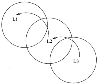
2-1 A set diagram of the TLA. Two of languages (L1-L3) are shown as overlapping if they are neighbors (one parameter value away) and have

some sentence patterns in common. . . . . 21

2-2 Niyogi and Berwick's [NB96a] Figure 1 with state 5 as the target. Arcs can exist from state to another only if there is data to drive the learner

to change states. Numbers on the arcs are the transition probabilities. 23

3-1 Time for rewritten local maxima search as a function of the number of

param eters. . . . . 39

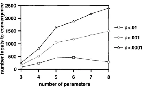
4-1 Average convergence times for languages without local maxima in 3-8

(10)

(11)

List of Tables

3.1 Parameters and setting values . . . .

4.1 Parameter settings for various languages . . . .

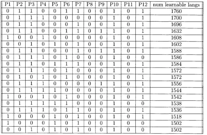
A.1 Best initial settings of 12 parameters (producing the highest number

of learnable languages) . . . .

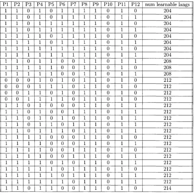
A.2 Worst initial settings of 12 parameters (producing the least number of

learnable languages) . . . .

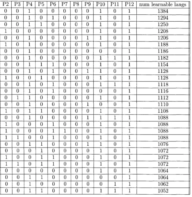
B.1 Best initial settings of 11 parameters (producing the highest number

of learnable languages) . . . .

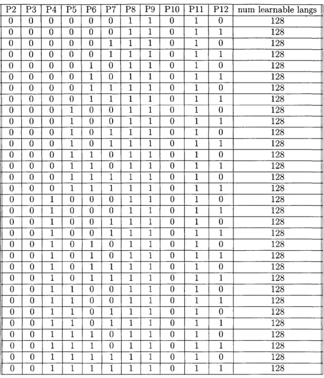
B.2 Worst initial settings of 11 parameters (producing the least number of

learnable languages) . . . .

B.3 Worst initial settings of 11 parameters (continued) . . . .

30 46 68 69 74 75 76 77 78

(12)

(13)

Chapter 1 Introduction

The problem of language acquisition is to describe how a child learns her first lan-guage. Of course, there are many different aspects of this process and questions to be considered, such as the sound system, word meanings, and syntactic rules. This the-sis will analyze an algorithm for acquisition of the child's syntactic knowledge which describes what kinds of steps a child takes on her way to learning the adult language and why she makes such steps.

Some of the key questions about syntax acquisition include:

(1) (i) what kind of input does the child receive

(ii) what kind of input does she actually use

(iii) what kinds of mistakes do children make and what can they tell us about language

(iv) how long does it take a child to learn a particular phenomenon

(v) what kind of algorithm does the child use so that she will eventually arrive

at her adult language

(14)

partic-ular, this thesis studies an implementation of Gibson and Wexler's [GW94] Trigger-ing LearnTrigger-ing Algorithm (TLA). I will start outlinTrigger-ing in this chapter the framework in which the TLA is studied (Principles and Parameters). Next I will give some background on this algorithm as well as other algorithms for language acquisition in Chapter 2.

In Chapter 3, I will describe the previous implementation of the TLA. as well as my enhancements to this work. Chapter 4 will describe some of the problems with the TLA and what the results might tell us about language and its acquisition. Chapter

5 provides ideas towards future work along several lines.

1.1 Principles and Parameters

A theory of language acquisition must describe how a child learns the various parts

of language. Those pieces must be defined with respect to some linguistic theory.

For this study, we will use the framework of Principles and Parameters as described

by Chomsky [Cho81]. In addition to a lexicon, or dictionary, for a particular

lan-gauge, this theory assumes a set of principles and a finite number of parameters. The principles are common to all human language and are therefore considered "innate" or at least they are known prior to a very early age. The parameters define the varia-tion among possible languages. All parameters are present in each language, but each parameter can take on a different setting. For example, English direct objects appear after the verb, but Japanese objects appear before the verb. The parameter which controls this fact is the Complement-Head order parameter, which will be discussed more later. The parameter is present in both English and Japanese, but its settings are reversed. The setting of all the parameters will produce a set of possible sentence patterns which will be the grammar for that language.

(15)

1.1.1 Principles

Since the principles are assumed to be innate, there is no learning involved. So I will not go into depth about many of the principles. Some of the principles include X-bar Theory, Case Theory, Theta Theory, Movement, and Binding Theory. For more details on these, see [Cho8l] and [Cho95].

1.1.2 X-bar Theory

X-bar Theory describes the hierarchical formation of sentences from phrases. X-bar Theory unifies the structure of all phrases, whether they be a noun phrase, a verb phrase, or any other phrase. Every phrase has a core element, or head. In a noun phrase the head is a noun, in a verb phrase it is a verb.

X-bar theory states that every phrase must have a head. And it determines how the phrases themselves are formed. The components of a phrase (XP), which is itself

hierarchical are the head (X0_{), the X-bar level (X'), the specifier (another phrase),}

and the complement (yet another phrase). There exists a set of rules to which every phrase must conform:

(2) (i) XP -> YP X' X' YP where YP is the specifier of the XP

(ii) X' -> X' YP | YP X' where YP is an adjunct to the XP

(iii) X' -+ X0 YP | YP X0 where YP is the complement of the XP

These rules assume binary branching. Haegeman [Hae9l] discusses the fact that if rules must branch this way only, then the grammar is more constrained. If a child hears an input string, she can parse it into fewer structures with binary branching than if she were allowed to have any number of branchings. If she has fewer possible

(16)

structures, it will be easier for her to decide among them. In this way, the acquisition of grammar will be much faster.

The rules also allow each of the two elements on the right hand side to be ordered in either way. This ordering is one of the ways languages can vary. Parameters controlling this ordering for every phrase in a particular language will be discussed below in the next section.

1.1.3 Parameters

Parameters will be assumed to take on binary values only. It is the acquisition of these parameter settings that this thesis will cover.

An example of two parameters is given below. Here we have two parameters, Spec-Head, and Comp-Head. These parameters determine the structure of any phrase. In X-bar theory, a phrase, or XP, is composed of two parts in any order: a specifier

and an X-bar level. The X-bar level, in turn, is composed of a head (X or X0

₎

and a complement in any order. The Spec-Head parameter determines whether the specifier or the X' appears first, and the Comp-Head parameter determines whether the complement or the head appears first. These settings apply to all phrases whether they be NPs, VPs, PPs, or any others. In the tree structure below, we have the

parameters set as Spec-first and Comp-final (= Head-initial).

(3) XP

Spec X'

(17)

Note that these are the settings for English. If the subject is the specifier of the verb phrase and the direct object is the complement, then we get the Subject-Verb-Object

(SVO) pattern that we see in English. These two parameters determine the basic

word order in any language.

We do not know the complete set of parameters, but we do believe that they should produce the general set of sentence patterns we should find for a particular language. They may alter the word order of a sentence by movement in some constrained way, determine where certain elements are place, or omit certain elements of a sentence.

1.2 Acquisition of a P & P grammar

In the Principles and Parameters framework, we have three components for the gram-mar of each language:

(4) (i) Principles

(ii) Parameters

(iii) Lexicon

We have stated that the principles are innate. Therefore there is no learning necessary for them. This thesis will not cover acquisition of the lexicon although there may very well be lexical parameters to learn.

This research covers the problem of acquisition of parameter settings for natural languages. Every child is believed to be able to learn any given language. This means that no matter what her genetic endowment is, she can acquire any possible natural

(18)

language (given assumptions that she will hear proper input). She is not pre-wired for any particular language.

How, then, can the process of learning the correct parameter settings be described?

If a child starts in an initial state (setting of parameters), how does she eventually

reach her final state?

The parameters we are talking about determine word order for a particular language. From these settings, we can derive the set of sentence patterns for that language. Pre-sumably these sentence patterns are what the child pays attention to in determining parameter settings.

The next chapter will describe a few kinds of algorithms proposed to capture this process. The Gibson and Wexler (1994) model, which is the on being investigated here, will be discussed thoroughly.

(19)

Chapter 2 Theories of Parameter Acquisition

As already mentioned, it is possible to propose many kinds of algorithms in order to describe the acquisition of parameter settings. Algorithms can differ in what they assume a learner is paying attention to in the language she hears. All do assume no negative evidence; the child does not learn from grammatical correction.

This chapter will give background on the TLA as well as a few other models of parameter-setting. For more of a description and analysis of the first three models, see Broihier [Bro97].

2.1 Triggering Algorithms

This thesis studies a type of algorithm involving triggers. Triggers are sentences that the learner cannot parse and which cause her to change her grammar hypothesis to a new hypothesis (setting of parameters). A triggering algorithm will describe how and when such a change can be made so that the learner will eventually arrive at her target adult language.

(20)

2.1.1 The TLA

Gibson and Wexler's [GW94] Triggering Learning Algorithm (TLA) proposes that the child changes parameter values one at a time when presented with a trigger. The TLA is stated in Gibson and Wexler [GW94] as follows:

(5) Given an initial set of values for n binary-valued parameters, the learner

at-tempts to syntactically analyze an incoming sentence S. If S can be successfully analyzed, then the learner's hypothesis regarding the target grammar is left un-changed. If, however, the learner cannot analyze S, then the learner uniformly selects a parameter P (with probability 1/n for each parameter), changes the value associated with P, and tries to reprocess S using the new parameter value.

If analysis is now possible, then the parameter value change is adopted. Other-wise, the original parameter value is retained.

The two constraints contained in this algorithm are the Single Value Constraint, given in (6i) and the Greediness Constraint, given in (6ii).

(6) (i) The Single Value Constraint

Only one parameter at a time may be changed between hypotheses.

(ii) The Greediness Constraint

The learner adopt a new hypothesis only if it allows her to analyze input that was not previously analyzable.

Niyogi and Berwick [NB96a] classified the TLA as having the properties shown below in (7):

(7) (i) a local hill-climbing search algorithm

(21)

(iii) no noise

(iv) a 3-way parameterization using mostly X-bar theory

(v) memoryless (non-batch) learning

Figure 2-1 below shows languages as neighboring (overlapping) sets. We will assume Li is the target. If the learner assumes an L2 grammar, she will transition to Li if she hears input from the non-overlapping area in L1. If she hears input from the intersection of Li and L2, she will remain in L2. If the learner assumes an L3 grammar, she will transition to L2 if she hears input from Li which is not in L3 and is in L2.

L1

L2

Figure 2-1: A set diagram of the TLA. Two of languages (Li-L3) are shown as overlapping if they are neighbors (one parameter value away) and have some sentence patterns in common.

2.1.2 Local Maxima in the TLA

In their paper, Gibson and Wexler studied a small, 3-parameter space. The three parameters included Spec-Head, Head, and V2. The Spec-Head and Comp-Head parameters have already been discussed. The V2 (or verb-second) parameter, if set, requires the finite verb to move from its base position to the second position in root declarative clauses.

(22)

In examining this three-parameter space, Gibson and Wexler found that there were some targets which were not learnable if the learner started out from a particular state or set of states. If there was no trigger to pull the learner out of a particular non-target state, this state was called a local maximum. If the learner ever reaches such a state, there is no way she can ever reach the target language.

In the three-parameter space, there were three out of the eight possible targets which had local maxima. Gibson and Wexler noticed that these three targets were all -V2 languages and the local maxima for them were all +V2 languages.

To solve the problem of local maxima, Gibson and Wexler proposed that the learner must start with some parameters having a default initial value. For this space, that would mean that the V2 parameter was initially set to -V2, while the other parameters could be set to any value initially. Since no +V2 languages had local maxima, these could be learned no matter what the initial state. For -V2 languages, the learner

would not be allowed to transition to a

+V2

language for a certain time, t.

However, Niyogi and Berwick [NB96a] and [NB96b] noticed that for Gibson and Wexler's three-parameter space, it was still possible, though not guaranteed, for the learner to transition to a local maximum even if she started in a -V2 state. This means that there was still some chance that the learner would not converge on her target language. Safe states are defined as those languages from which it is not at all possible to arrive in a local maximum.

The example Niyogi and Berwick gave is shown below in Figure 2-2. Here, the target is a Spec-first, Comp-final, -V2 language such as English. The arcs represent possible transitions, with their probabilities, as will be discussed later. Any state with no outgoing arcs is called an absorbing state. Of course, the target will always be an absorbing state. When the learner enters the target, she can never leave it because the input she hears will be only from the target. Any absorbing state which is not the target language is a local maximum. Also, any state which has outgoing arcs only to

(23)

local maxima is also a local maximum. So in the diagram with state 5 as the target, state 2 is an absorbing state and maximum and state 4 is a maximum also.

41/12 [1 0 1] 1/12 31/36 1/12 1 1 0] 3 [1 0 0] 6 18 1/3 2 sink sink target: 5 5/18 5 [s ec 1st, comp final, -V2] 76 [0 1 0] 6 1 ] 2/3 1 _5/6 1/18 1/36 1/12 [0 0 1] 8 8/9

Figure 2-2: Niyogi and Berwick's [NB96a] Figure 1 with state 5 as the target. Arcs can exist from state to another only if there is data to drive the learner to change states. Numbers on the arcs are the transition probabilities.

Note that this diagram shows for other states that it is possible though not guaranteed to transition to a local maximum from a -V2 language. The two cases here are from state 3 to state 4 and from state 1 to state 2. These transitions are not the only ones, but they are possible, leaving the learner in a state from which she can never learn her target adult language.

(24)

2.1.3 Triggering as a Markov Process

Niyogi and Berwick [NB96a] describe how to model finite parameter learning as a Markov chain. A Markov transition matrix A is a matrix with the following two properties [Str93]:

(8) (i) Every entry of A is nonnegative.

(ii) Every column of A adds to 1.

Niyogi and Berwick have every row of A adding to 1 instead for ease of understanding. For each target grammar in a space, we can build a transition matrix that tells the probability of transitioning from one state to another. The entry (ij) is the probability

of transitioning from state i to state

j

for the given target.

Niyogi and Berwick show how to determine the probability of transitioning from one state to another. The probability of flipping a single parameter value chosen at random is 1/n for n parameters. And the probability of hearing an input which will cause this flip is the sum of the probability of hearing a string sj over all strings sj in the target language which are not in the language of state s but are in the language of state k. Thus, the probability of a transition from state s to state k can be stated as:

P[s -+ k] (1/n)P(sj)

SjELt,sjgLS,Sj ELk

Of course, we are interested in only transitions between neighboring states. A

neigh-boring state of state s in this model is one which differs from s in one parameter setting only. Since the formula above gives only the probability of transitioning out of a current state, we must also find the probability of remaining in the current state.

(25)

All probabilities must add to 1, so the probability of staying in a state is P[s -+ s] = 1 - E P[s - k]

k a neighboring state of s

If we assume an even distribution for the sentence patterns, then we have P(sj) =

1/ILt|, where |Lt| is the number of patterns in the target language.

Given the transition matrix, we can determine local maxima for a particular target

language. The matrix Ak gives the probability of being in a certain state after taking

k steps. As we take k to infinity, Ak will converge to a steady state. From this steady state, we will be able to read off the local maxima and safe states. Recall that a safe state is one that from which the learner will reach the target with probability 1. Then the safe states will be those rows which contain the value 1 in the column of the target language. The local maxima are those from which the learner cannot reach the target; their rows will have a value of 0 in the column of the target language. The non-safe states will be all the rest; their rows have a value between 0 and 1, exclusive, in the column of the target. That value will give the probability of reaching the target even though there will not necessarily be convergence to the target.

Modelling the TLA as a Markov chain allows us to retrieve more information about the process. We can also use the transition matrix to compute convergence time for a target. Of course, since states with maxima do not necessarily converge to the target, we can measure convergence time on only those states which have no local maxima.

Niyogi and Berwick give the following theorem from Isaacson and Madsen [IM91]:

Theorem 1 Let T be an n x n transition matrix with n linearly independent left

eigen-vectors x1,... xn corresponding to eigenvalues A,,.. ., An. Let ,ro (an n-dimensional row vector) represent the starting probability of being in each state of the chain and ,F (another n-dimensional row vector) be the limiting probability of being in each state.

(26)

by

|

?oT' -7 11-1 ZA'1oyiXi

1

max fAi k 170yXi |}

i=2 -<~ - i=2

where the y 's are the right eigenvectors of T and the norm is the standard Euclidean norm.

If we find that it takes an extraordinarily large number of transitions to end up in the

target state with a probability of one, then we can say that this is not a reasonable theory of parameter setting.

2.2 Cue-based Algorithms

Dresher and Kaye

[DK90]

proposed an algorithm for setting phonological parameters.

Their kind of algorithm is referred to as a cue-based approach. This kind of algorithm does not assume that the learner is reasoning about settings of parameters. Rather, the inference tools are pre-compiled, or hard-wired into Universal Grammar. The learner is provided with cues which tell her what patterns to look for in the input and what conclusions about a parameter setting to make when these patterns are found. Every parameter or parameter setting is associated with a particular cue. Every parameter has a default value. There may be an ordering about which parameters are set; this will represent dependencies among parameters. If a parameter value is set to a new value, all parameters which depend on it must be reset to their default values.

We saw that cues were stated as one per parameter or parameter setting. We know that parameters can interact and they will moreso with larger spaces. With large numbers of parameters, it seems necessary to define multiple cues for each parameter setting, depending on the settings of other parameters. Even with the partial ordering, it is highly unlikely that we can get away with one cue per parameter setting while

(27)

ignoring the other parameter settings.

Unlike the TLA, this cue-based algorithm requires the memory of previous input sentences. The learner needs to know whether she has seen a particular pattern or set of patterns in the input before she can set a certain parameter value. How far back must her memory go and is that reasonable? Certainly holding a few input sentences in memory does not sound so unreasonable. But it is probably necessary to hold many more than that if certain cues are defined so that the learner needs to have heard all the different sentence patterns in a certain set. If that is the case, the learner could need a large memory for so many previously heard sentences. It seems rather unlikely that a child would be able to have such a large memory to hold

enough previous utterances.

2.3 Structural Triggers

Fodor [Fod97) proposed the Structural Triggers Learner (STL) algorithm. In this algorithm, the learner is assumed to use only a parser, which she needs anyway. Upon receiving an input sentence, the learner superparses it, or parses it with all possible grammar which come from varying the unset parameters. On examination of the grammars which can parse the input, the learner can attempt to set parameters.

If all grammars which parse the input sentence have parameter P set to value V, then

the learner adopts that parameter setting. Each time a parameter is set, the number of possible grammars for the learner to use shrinks until eventually all parameters are set.

Bertolo et al. [BBGW97] have shown that the STL is really an instance of a cue-based learner. Instead of having pre-compiled cues, the STL derives its cues as the result of superparsing.

(28)

there are n binary parameters, there are 2' grammars when the learner begins with no parameters set. For each input sentence, the learner must try to produce as many parses as there are grammars. With 2' grammars, this seems like an awfully large amount of computation and memory to store all output parses to be compared.

2.4 A Variational Theory

Yang [Yan99] proposed a rather different approach to parameter setting. The models discussed above were transformational models; the learner moves from one grammar to another. Yang proposes that the child has more than one grammar in competition at a time.

Since the child has a population of grammars, we need to know how she chooses a particular grammar to use and how she eventually chooses the one identical to the target adult grammar. Yang suggests that each grammar is associated with a proba-bility, or weight. The probability value for each grammar may be adjusted depending on the input. It can be either increased (rewarded) or decreased (punished). For an input sentence, a grammar is chosen with the probability currently assigned to it. If the grammar chosen can analyze the input sentence, the grammar is rewarded and the other grammars are punished. If the grammar chosen is not able to parse the

sentence, then it is punished, and all other grammars are rewarded.

Yang shows that this algorithm is guaranteed to converge to the target adult grammar and that it makes correct predictions about the timing of certain linguistic phenomena of child language acquisition. Eventually a single grammar will have a high enough probability associated with it that the others will have to die off.

This algorithm requires the learner to store a probability value with each possible grammar. Again there are 2' grammars for n binary parameters. The initial proba-bilities associated with each grammar will be quite low for larger values of n.

(29)

Chapter 3 Implementation

The TLA has been implemented in Common Lisp in order to study the space and its problems more carefully. Gibson and Wexler's proposed solutions to the local maxima problem can now be investigated more thoroughly. It will be possible to determine how important this problem could be in a more realistic space with a larger number of parameters. This chapter describes an original implementation and the enhancements that this research project has made to the system.

3.1 Original system

Stefano Bertolo has implemented a system which is useful in studying the TLA at a greater depth. Instead of using just the three parameters in Gibson and Wexler, Bertolo adds nine more parameters and generates the larger space of 12 binary

param-eters. His program generates sentence patterns for each of the 212 (= 4096) settings

of the parameters. From these sets of sentence patterns, it searches for the set of local maxima and the set of safe states for each target.

(30)

3.1.1 Parameter set

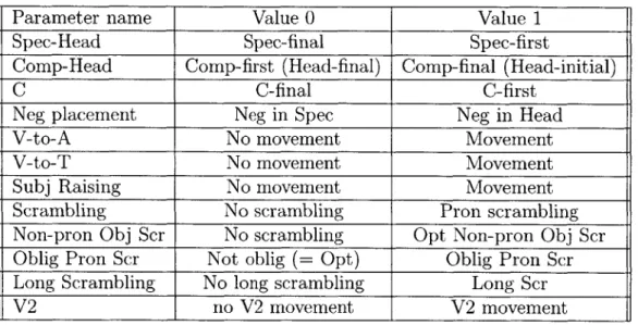
The set of 12 parameters used in this system is listed below in Table 3.1 with the meanings of their values:

Table 3.1: Parameters and setting values

Parameter name Value 0 Value 1

Spec-Head Spec-final Spec-first

Comp-Head Comp-first (Head-final) Comp-final (Head-initial)

C C-final C-first

Neg placement Neg in Spec Neg in Head

V-to-A No movement Movement

V-to-T No movement Movement

Subj Raising No movement Movement

Scrambling No scrambling Pron scrambling

Non-pron Obj Scr No scrambling Opt Non-pron Obj Scr

Oblig Pron Scr Not oblig (= Opt) Oblig Pron Scr

Long Scrambling No long scrambling Long Scr

V2 no V2 movement V2 movement

The first three are basic word order parameters that are needed for all phrases while the rest involve movement. The only exception is Neg placement, which does not involve movement, but it is not necessary for the formation of all kinds of sentence patterns the way the Spec-Head, Comp-Head, and C-placement parameters are.

A note needs to be made about the scrambling parameters (8-11). Parameter 8 is

the general scrambling parameter, which allows object pronoun scrambling. Only if scrambling is allowed (by parameter 8) are other types of scrambling allowed, as

described by parameters 9-11. So the settings of parameters 9-11 are ignored if

parameter 8 is set to 0 (no kind of scrambling allowed). So we have four parameters which could then be set 16 different ways. If we have a scrambling language, we have all 8 possible settings producing different languages. But if we have parameter 8 set to

0, we have only one language. So we really have only 9 of the sixteen different possible

(31)

9/16 of that, or 2304, possible different languages.

3.1.2 X-bar structures

The program creates basic sentence patterns from X-bar templates and from the settings of the three word order parameters. Then it sequentially applies to these X-bar structures the operations of the settings of each of the other 9 parameters. Finally, the structure is removed in order to find the set of sentence patterns. This makes sense, of course, since children do not receive input sentences with structures; rather they hear simply an input string of words and try to parse it themselves.

The X-bar templates include such categories as CP, TP, AP, NegP, Aux, VP, Adv,

Obj, Obj1, Obj2, Prep, E-sentence, and Comp. These allow for constructions

op-tionally containing auxiliaries, adverbs, and negation. Verb phrases may contain no objects, one object, two objects, or an object with a prepositional phrase. Both declarative sentences and imperative sentences are allowed by declaring that the root of the sentence can be either CP or VP.

3.1.3 Formation of the space

The formation of the parameter space takes place with sequential application of each of the parameter functions. The initial 3-parameter space is created first. The infor-mation of the list of sentence patterns for a language (parameter setting) is written to a file for each language. Then the parameters are applied sequentially. The applica-tion of each parameter takes a file from the previous space, extends it with the 0 and

1 settings and writes the sentence patterns corresponding to each of these settings to

each new file.

(32)

state produces exactly the same set of surface patterns, these states are grouped together to form a cluster. The whole 12-parameter space, with sentence patterns

encoded, is stored to a separate Lisp file.

Finally, a Huffman code is established for the space, and the sentence patterns are converted to decimal numbers from this Huffman code. Storing the sentences as decimal numbers allows for faster processing in the next stages. It is easier to compare numbers than lists of strings. The Huffman code information is stored in a Lisp file.

In this 12 parameter space, there are 212 possible languages from the various settings of the parameters. However, there are not 4096 different sets of sentence patterns produced from this system. In fact, there are only 1136 clusters with distinct sets of sentence patterns. Note that this 1136 is much smaller than the number we would expect even when we count as one the states having parameters 1-7 and 12 set iden-tically, parameter 8 set to 0, and parameters 9-11 set to any value. That value would

be 4096 * 9/16 - 2304.

3.1.4 Local maxima search

From these states and their corresponding set of sentence patterns, triggers can be determined when a target state is known. Then local maxima and safe states can be determined by comparing sets of surface patterns of neighboring states. These clusters with their maxima and safe states are output to files.

The neighboring states were calculated by finding the states that were within a certain distance away. The distance to be studied could be set to any value. Gibson and Wexler required that the distance not be more than 1. The setting of this value would allow other options to be explored, but this was not done here.

The algorithm Bertolo used to find the maxima was also used to find the safe states. Given two sets, set1 and set2, the routine determines which of the states in set2 have

(33)

no path to at least one state in set1. The algorithm can be stated generally as follows:

(9) (i) Set1 := Lt

(ii) R = set of states in Set2 which neighboring states in Set1 that do have

transitions to an element in Set1

(iii) Set1 := Set1 U R

(iv) Set2 := Set2 - R

(v) go to step (ii) if R is not the null set

(vi) OutSet := Set2

For the maxima search, set1 starts off containing only the target language(s). And set2 contains all the other languages. Then the maxima will be those that have no path to any of the target languages.

For the safe state search, set1 starts as containing the maxima just found and set2 contains all languages except the maxima and the target(s). Safe states are those which have no path to any maxima, so this algorithm does the trick. After this

algorithm runs, the maxima are simply OutSet (= Set2). But the set of safe states

is the union of the OutSet with the set of targets (since these are always safe).

3.1.5 Running time

The approximate time which Bertolo had reported for the running of the algorithm on a Sparc 20 is as follows:

(10) (i) 3 hours to create the space from scratch for the 12 parameters

(34)

3.2 Enhancements to the system

This section will describe the enhancements that were made to the system for this research project. Many of the enhancements were made in order to make the program more useful in general cases. If it becomes more flexible, then it allows more apects of the TLA to be studied. There were two main enhancements made to allow the program to be more general:

" allow the users to restrict the parameter space from the set of twelve parameters by allowing them to select the parameters they are interested in studying " allow for easy addition of new parameters so that the space can be expanded

also

A third improvement made was to decrease the time of the maxima search. Recall

that Bertolo's implementation required about 30 minutes to find the maxima and safe states for each target language. I rewrote the algorithm for the search for local maxima more efficiently. This running time for the maxima search for each language was significantly reduced even though the total time for all languages is still quite long.

The last major enhancement was to model the triggering process as a Markov chain. We have already described how maxima and safe states can be found from this rep-resentation. This method has been implemented as has the method for finding con-vergence times given a Markov chain.

3.2.1 Selection of parameter space

We decided to allow for the selection of a set of parameters to be studied. Gibson and Wexler proposed that one solution to the problem of local maxima might be that

(35)

the parameter space was not correct. Certainly their three-parameter space was too small to be condidered realistic. Perhaps the correct parameter space would not have the problem of local maxima, assuming the correct parameter space could even be found. If the user can choose the parameter space to be explored, then he can run the program on each different space he chooses and examine the results to find which targets in which spaces have local maxima.

The first enhancement made to the Bertolo system was a utility for selection of parameters to study. As mentioned previously, the first three word order parameters were used to create a small space and then the rest of the parameters were applied sequentially, creating larger and larger spaces until the complete 12-parameter space was created.

As before, the three word order parameters are required to start with. The space for these parameters is created and then expanded depending on what other parameters may be selected. Therefore, the minimum space to be explored is this 3-parameter space.

My selection routine takes as input the list of the functions that do the application

of each of the parameters. This list is broken down into four groups according to the kinds of parameter. One set corresponds to the scrambling parameters. Another corresponds to the parameters that most easily apply to surface forms, as will be discussed below. Yet another is the set that will apply just before the surface param-eters do, the last stage of application of structural paramparam-eters. The last set contains all the rest that can be applied sequentially.

Global variables are used to define the sets of possible scrambling parameters, possible final structural parameters, and possible surface parameters. The union operation is used on each of these possible sets and the list of selected parameters in order to separate the selected parameters into the appropriate sets.

(36)

set of general parameters are applied sequentially, increasing the space each time. Next, it is determined whether the main scrambling parameter was contained in that general set. If not, no other scrambling parameter is applied, even if it had been selected. If the main scrambling parameter was selected, then the space is increased

by applying the other scrambling parameters. Once the scrambling parameters have

been applied (if necessary), then the final structural parameters (in this case, just V2) can be applied. Finally the X-bar structure is removed from the sentence patterns and the space consists of flat sentence patterns for each target. Then the last set of parameters (if it contains any) can be applied since they apply most easily to surface patterns.

After this application, the space can be compacted as before and the rest of the process of looking for maxima and safe states can continue.

3.2.2 Addition of parameters

Now that it is possible to select sets of parameters instead of having to study exactly the original twelve, we want to make it easy to add new parameters so that more spaces can be studied. This addition could be important if there was another parameter thought to be important or helpful in distinguishing language patterns.

In order to add a new parameter, it is necessary for the user to define a function that describes how each setting of the parameter may or may not alter the structure of the sentence pattern. It is also necessary to determine which type of parameter this new one is. It may be a parameter of the usual type, it may be a scrambling parameter, or it may be one defined to apply to surface patterns. If the new parameter is either a scrambling parameter or a surface parameter, then its function name must be added to the list of parameters for the respective global variable.

(37)

them has been studied yet. The previous system generated only simple sentence patterns, whether they be declarative or imperative. But one might also want to include questions since children must hear many kinds of questions. We decided to add parameters for questions involving subject-auxiliary inversion and Wh-movement since these can be crucial to the formation of questions.

We decided that it was easier to define a subject-auxiliary operation in terms of a surface pattern than to define it to produce the whole structure showing the proper movement. The function for the Subj-Aux inversion parameter simply takes a set of sentence patterns and searches for any pattern containing a SubjO followed by AuxO. It then adds to the set of sentence patterns another sentence pattern identical to the first except with AuxO followed by SubjO instead of the original non-inverted pattern with SubjO followed by AuxO.

For the Wh-movement operation, this was easier to implement with the complete X-bar structure for each sentence pattern. Therefore this was not a surface parameter; rather it was the general type of parameter. This operation examined each sentence pattern in the target language and added Wh-questions that could be formed from it. This parameter function substituted a Wh in for any of the following categories:

SubjO P-ObjO ObjO P-Obj1-O Obj1-O Obj2-0 AdjunctO Adv. Then each setting of

the parameter was considered. For the setting of 0, the sentence patterns with Wh substituted were left unchanged because Wh-words stay in situ for these languages. For the setting of 1, the Wh-word is moved to Spec-CP and a trace is left because Wh-words are required to move in these languages.

Another new parameter thought to be useful is pro-drop. If set, this parameter allows the dropping of personal pronouns in language. Most commonly it is the subject since pronouns occur in subject position most often. As an example of the variation allowed

by this parameter, we look at the differences among a few languages. English does

not allow pronouns to be dropped in general, but languages like Italian drops them quite freely, and Chinese allows them to be dropped only in certain cases. We know

(38)

that there is a long stage in child language that English-speaking children often omit subjects, first noted by Bloom [Blo70].

Most commonly it is the subject since pronouns occur in subject position most often. We therefore decided to implement this parameter as simply a subject drop param-eter rather than a general pro-drop paramparam-eter This paramparam-eter describes an optional dropping of the subject if set to 1. No dropping is allowed if set to 0. The imple-mentation of this parameter was also most easily done from the surface form. If a sentence was found containing a subject NP, then another sentence was added to the list of sentence patterns for that particular language with the subject omitted.

Since we have shown that it is easy to add these three new parameters, it would also be easy to add others. One first needs to decide if a new parameter is a special type (scrambling, surface, or final structural). If so, its function needs to be added to the appropriate global list of these parameters. The definition of the parameter application function needs to define the affect of each of the 0 and 1 settings.

3.2.3 Rewriting of maxima search

Since most of the running time of Bertolo's program came from the maxima search,

I decided to rewrite it to be more efficient. From 3.1.4, it can be seen that Bertolo's

implementation looked back from every non-maximum for states that could transition to it. This is quite a bit of computation every time even though the space to search through became smaller each time.

I decided to determine the set of transitions for once and for all at the start of maxima

and safe state search. Then I could use this information to find the set of maxima and the set of safe states. Otherwise, my implementation was quite similar to Bertolo's but the complete set of possible transitions are computed only once per target language. Given that the safe state is a non-maxima, it finds all the states that lead to it in this

(39)

set of transition pairs. Just as Bertolo's did, the set of non-maxima was increased in this way until it stopped growing. And the search for safe states was done similarly to Bertolo's also.

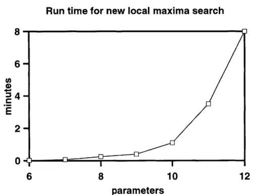
When the search for local maxima was written this new way, it computed all the pos-sible transition pairs first, instead of for each iteration through the search recursion. The complete set of transition pairs will be useful for the improvements described next. Computing transitions only once significantly cut down the running time of this algorithm even though this is still the majority of the computation involved in the search. Where this part of the program used to take about 30 minutes per 12-parameter language, it now takes only about 8 minutes per language, on average. Graph 3-1 below shows the time for the new algorithm as a function of the number of parameters. The time can be seen to be increasing exponentially since the size of the space is also increasing exponentially.

Run time for new local maxima search 8- 6-(n

2-0

6 8 10 12 parameters

Figure 3-1: Time for rewritten local maxima search as a function of the number of parameters.

(40)

3.2.4 Markov method for maxima and safe states

We also decided to model the TLA as a Markov process as described in section 2.1.3. This allows us to find local maxima and safe states for any target language.

In order to use this method, we need transition probabilities between every two states with respect to a given target. The routine mentioned in the section above required finding the set of all transition pairs with respect to a certain target. I extended this routine so that along with all such transition pairs, it would return the proper probability values necessary for the Markov matrix. With each pair of languages which have a transition from the first to the second, it returns the number of triggers that would cause such a transition and the number of sentence patterns in the target grammar. Recall that, for an even distribution among input sentences, the probability of transition can be stated as

1 ItriggeringsentsI

n |Lt|

The routine to find transition pairs worked only to find a transition from one state to another different state. So the probability of remaining in one state was not calculated. I wrote another routine to take the set of transition pairs and find this probability. It added the probabilities of leaving a certain state and subtracted this from 1 in order to find the probability of staying in that state. So now there was a full set of transitions and their probabilities.

We decided to perform the matrix manipulations in Matlab. However, the data needed to be retrieved from the parameter space, which was all represented in Lisp. I wrote yet another version of the maxima search routine in Lisp to calculate the transition probabilities and output a file that could be run in Matlab. This file contained the definition of the Markov transition matrix and a call to the routine which finds the maxima and safe states from the transition matrix.

(41)

In the first attempt to define the matrix, I had Lisp calculate each row and then write it out to a Matlab (.m) file. When I loaded the Matlab file, and ran the maxima and safe state search function, it worked fine for small for small values of parameters, but Matlab quickly ran out of memory for the 12-parameter space. This is because a matrix for 12 parameters has dimensions of 4096x4096. It is even worse than just this because this matrix has to be raised to a higher power until it converges to a steady state matrix so there is multiplication of two 4096x4096 matrices. In order to solve this problem, I needed to represent the matrices as sparse matrices. This was possible because most entries of these matrices are 0 since there are few transitions between states. For a space of n parameters, a particular state can transition to at most n states since neighboring states are those that are 1 parameter setting away.

Now the Lisp routine writes out a Matlab file containing a definition of a sparse matrix containing all zeros initially. Then each transition probability is filled in separately. Finally, the Matlab file contains a call to the function to find the maxima and safe states.

The algorithm for finding the maxima and safe states described by Niyogi and Berwick was stated in section 2.1.3 above. In implementing it for this space, I had to make minor adjustments to accommodate the system here. The first part of the algorithm involved multiplying the matrix by itself until a steady state was reached. In my implementation, I repeatedly squared the matrix until each element was within a certain difference range from the previous matrix. Here, I used the value of .0001 for a test of convergence.

Recall that if a language was a maximum for a particular target, its entry in the target column would be zero. The difference I ran into for this is that we have clusters of targets in this system. The languages in this cluster are all targets, so there is no single target column to examine in the steady state matrix. My implementation summed the entries for that row in all the target columns. If that sum was 0 (or

(42)

The set of maxima were collected in an array and output from the maxima function.

Similarly, the cluster problem arose when trying to find the safe states from the steady state matrix. Recall that a state was safe if it was guaranteed to end up in the target state. In Niyogi and Berwick's description of the Markov model, this meant that the entry for the state's row in the target column had to have a value of 1. Again, if we have multiple equivalent languages in a cluster, we have no single column to examine. Of course, we cannot even examine each entry for a value of 1. Instead, all the entries in the target columns for that state's row must add to a value of 1. My function looped through the array of target languages and summed the values in their entry for each language row. If that sum for each row was 1 (or rather the difference

between 1 and that sum was < .0001), then the state was considered safe. An array

of all the safe states was output from the safe state function.

Of course, the states that are not maxima or safe states are considered non-safe states.

But these were not specifically calculated, so they were not output anywhere.

The maxima and safe states were output to a file for each target language. The format for this file was the same as Bertolo's format. It was a Lisp file including the target cluster in binary notation and the lists of the maxima and safe states in decimal notation. This file was formatted and output from Matlab at the end of this calculation. These files were output in Lisp as before so that they could be used for calculations using this information which will be discussed later.

The time for running this part of the program is shown below.

(11) (i) 8 minutes in Lisp to create each Matlab file

(ii) 12 minutes in Matlab to run a 12-parameter file

The total time of about 20 minutes per cluster is more than the 8 minutes of my rewritten Lisp maxima search. The majority of the time in Lisp is spent finding all

(43)

the transition pairs. This was necessary for the Lisp implementation of the local maxima search as well as for the output of a Matlab file. Then of course it take quite a bit of time to write out all the transitions to a Matlab file.

Although this total time seems large, the representation as a Markov model allows us to find more information about the space. Specifically, it allows us to find convergence times, which will be discussed in the next section.

3.2.5 Markov model for convergence times

Given the transition Markov matrix from before, we can now compute the convergence times for a matrix. The formula in Theorem 1 is repeated here. We will not used the term to the right of the < sign.

n n

goT - =H ZAroyixi < max fIAi kZ 1 7royzX II}

i=2 i=2

The problem is to find the value of k which allows for convergence. The probability of convergence must be (close to) the value of 1.

There are two different ways to implement this formula. The first is to simply use the 7roTk term. The second is to use the summation term just to the right side of the

= sign.

For the first way, ro was set to a row vector of length 2n of values 1/2", where n is the number of parameters in the space. Then the transition matrix A was raised to

increasing values of k until the entries in the columns of the target languages of qroTk

summed to a value within a certain distance from 1. With this implementation, the multiplication of T by itself caused Matlab to run out of memory sometimes. This happened only when the number of parameters was high, as for the 12-parameter

(44)

space. Even then, this did not happen for every matrix.

The second way to use this formula was used for the final implementation. This implementation does not multiply matrices. It does not even need to know which are the target languages. Let us see why. The left hand side of the equation takes the difference between -roTk and -r, which is the final probability of being in each

state. We cannot calculate what ir is when we have clusters with more than one

target language. But we do know that in the limit, it is of course the same as 7roTk. Therefore the difference will be a row vector of all zeroes, and its norm will be zero. Thus we can take increasing values of k until the norm of the summation on the right hand side is also within a certain range from zero. At that point we have found the value for k, the number of steps to convergence. Matlab calculated ro, the left eigenvalues and eigenvectors, and the right eigenvectors once since those did not depend on the value of k. Then value for k was increased and the sum and norm were calculated and tested to be within a certain distance from the value 1. When this norm was close enough to 1, the value of k was returned as the answer to the number of steps to convergence.

(45)

Chapter 4 A Study of the Parameter Space

This chapter describes what we have learned from the parameter space generated

by this program. We will give settings for attested natural languages which will be

used in verification of the algorithm's predictions. Next we will examine how bad the problem of local maxima really is in this 12-parameter space. We will also test some possible solutions or explanations. Finally, we will examine the convergence times for these larger spaces for plausibility.

4.1 Parameter Settings in actual languages

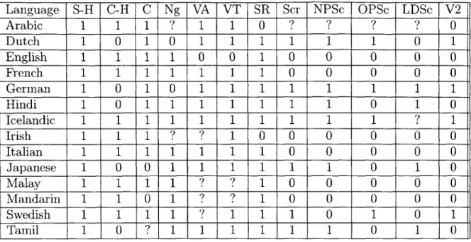
Table 4.1 below shows settings of each of the twelve original parameters for a few different languages. These settings were worked out by Anjum Saleemi. Of course some settings are questionable, but they may not always make a difference because languages with opposite settings for a particular parameter may sometimes cluster together. Note that when there was no scrambling at all in a language, parameter 8 was of course set to 0, and so were parameters 9-11 since we cannot really determine their settings.

(46)

Table 4.1: Parameter settings for various languages Language S-H C-H C Ng VA VT SR Scr NPSc OPSc LDSc V2 Arabic 1 1 1 ? 1 1 0 ? ? ? ? 0 Dutch 1 0 1 0 1 1 1 1 1 1 0 1 English 1 1 1 1 0 0 1 0 0 0 0 0 French 1 1 1 1 1 1 1 0 0 0 0 0 German 1 0 1 0 1 1 1 1 1 1 1 1 Hindi 1 0 1 1 1 1 1 1 1 0 1 0 Icelandic 1 1 1 1 1 1 1 1 1 1 ? 1 Irish 1 1 1 ? ? 1 0 0 0 0 0 0 Italian 1 1 1 1 1 1 1 0 0 0 0 0 Japanese 1 0 0 1 1 1 1 1 1 0 1 0 Malay 1 1 1 1 ? ? 1 0 0 0 0 0 Mandarin 1 1 0 1 ? ? 1 0 0 0 0 0 Swedish 1 1 1 1 ? 1 1 1 0 1 0 1 Tamil 1 0 ? 1 1 1 1 1 1 0 1 0

The parameter settings for these languages will be useful in testing how well the TLA really works. We know that these languages are certainly learnable.

sure that the TLA predicts them as such.

So we must make

4.2 Selection of Parameter Space

The selection of the parameter space did not make the problem of local maxima disappear. When only Gibson and Wexler's three parameters (Spec-head, Comp-head, V2) were examined, there were no maxima in this space. This can be attributed to the larger set of possible sentence patterns used in this implementation. Even in a space of four parameters (Gibson and Wexler's three plus C-direction), there were no local maxima.

Since the purpose of this project was to model a more realistic parameter space, it was necessary to select more than a few parameters to investigate. As soon as more

An analysis of finite parameter learning in linguistic spaces

An Analysis of Finite Parameter Learning in

Linguistic Spaces

by

Karen Thompson Kohl

Submitted to the Department of Electrical Engineering and Computer

Science

in partial fulfillment of the requirements for the degree of

Master of Science in Computer Science and Engineering

at the

MASSACHUSETTS INSTITUTE OF TECHNOLOGY

June 1999

©

Karen Thompson Kohl, MCMXCIX. All rights reserved.

The author hereby grants to MIT permission to reproduce and

distribute publicly paper and electronic copies of this thesis document

in whole or in part, and to grant others the right to do so.

A uthor...

Department of Electrical Engineering and Computer Science

May 17,1999

Certified by...

Professor of

Robert C. Berwick

Computex, Science and Engineering

Thesis Sjiriervisor

Accepted by...

A. C. Smith

An Analysis of Finite Parameter Learning in Linguistic

Spaces

by

Karen Thompson Kohl

Abstract

Acknowledgments

Contents

List of Figures

List of Tables

Chapter 1

Introduction

1.1

Principles and Parameters

1.1.2

X-bar Theory

1.1.3

Parameters

)

1.2

Acquisition of a P & P grammar

Chapter 2

Theories of Parameter Acquisition

2.1

Triggering Algorithms

2.1.1

The TLA

2.1.2

Local Maxima in the TLA

+V2

2.1.3

Triggering as a Markov Process

j

|

1

2.2

Cue-based Algorithms

[DK90]

2.3

Structural Triggers

2.4

A Variational Theory

Chapter 3

Implementation

3.1

Original system

3.1.1

Parameter set

3.1.2

X-bar structures

3.1.4

Local maxima search

3.1.5

Running time

₎