Development and experimental validation of direct controller tuning for spaceborne telescopes

Development and Experimental Validation of

Direct Controller Tuning for Spaceborne Telescopes

by

Gregory J. W. Mallory

B.Sc.Eng., Electrical Engineering, University of New Brunswick, 1994 M.Sc., Physics, University of New Brunswick, 1996

SUBMITTED TO THE DEPARTMENT OF AERONAUTICS AND ASTRONAUTICS IN PARTIAL FULFILLMENT OF THE DEGREE OF

DOCTORATE OF PHILOSOPHY at the

MASSACHUSETTS INSTITUTE OF TECHNOLOGY

June 2000

@ 2000 Massachusetts Institute of Technology, All rights reserved

Signature of Author ...

6epartmetof

/

Certified by

Certified by

Professor David W. Miller, Committee Chair Department of Aronautics and Astronautics

Professor Eric Feron Department of Aeronautics and Astronautics

Dr. Brent D. Appleby ,,,Charles Stark Drper Tabpratory

'Profeffor David H. Staelin Depprtyient of Electrical Engineering Certified by

Certified by

Accepted by .

MASSACHUSETTS INSTITUTE Professor Nesbitt W. Hagood IV OF TECHNOLOGY Chairman, Department Graduate Committee

S~p

0

2000

SFP 0

7 2000

Development and Experimental Validation of Direct Controller Tuning for Spaceborne Telescopes

by

GREGORY J. W. MALLORY

Submitted to the Department of Aeronautics and Astronautics on April 21, 2000 in Partial Fulfillment of the

Requirements for the Degree of Doctorate of Philosophy at the Massachusetts Institute of Technology

ABSTRACT

Strict requirements in the performance of future space-based observatories such as the Space Interferometry Mission (SIM) and the Next Generation Space Telescope (NGST), will extend the state-of-the-art of critical mission spaceflight-proven active control design.

A control design strategy, which combines the high performance and stability robustness

guarantees of modem, robust-control design with the spaceflight heritage of conventional control design, is proposed which will meet the strict requirements and maintain traceabil-ity to the successful controllers from predecessor spacecraft. Two principal tools are developed: an analysis algorithm that quantifies each sensor/actuator combination's effec-tiveness for control, and a design engine which tunes a baseline controller to improve per-formance and/or stability robustness.

The sensor/actuator effectiveness indexing tool requires a reduced-order state-space model of the plant. A modification of the balanced reduction method is introduced which improves numerical conditioning so that the order of large models of flexible spacecraft may be decreased. For each sensor and actuator an index is computed using the modal controllability from an actuator weighted by the modal cost in the performance, and the model observability of a sensor weighted by the modal cost of the disturbance. The special case of actuators that are used for active output isolation is handled separately. The

4 ABSTRACT

designer makes use of the sensor/actuator indexing tool to select which control channels to emphasize in the tuning.

The tuning tool is based on forming an augmented cost from weighting performance, sta-bility robustness, deviation from the baseline controller, and controller gain. The tuning algorithm can operate with the plant's state-space design model or directly with the plant's measured frequency-response data. Two differentiable multivariable stability robustness metrics are formed, one based on the maximum singular value of the Sensitivity transfer matrix and one based on the multivariable Nyquist locus. The controller is parameterized with a general tridiagonal parameterization based on the real-modal state-space form. The augmented cost is chosen to be differentiable and a closed-loop stability-preserving unconstrained nonlinear descent program is used to directly compute controller parame-ters that decrease the augmented cost. To automate the closed-loop stability determination in the measured-data-based designs, a rule-based algorithm is created to invoke the multi-variable Nyquist stability criteria.

The use of the tuning technique is placed in context with a high-level control design meth-odology. The tuning technique is evaluated on a sample problem and then experimentally demonstrated on a laboratory test article with dynamics, sensor suite, and actuator suite all similar to future spaceborne observatories. The developed test article is the first space-telescope-like experimental facility to combine large-angle slewing with nanometer opti-cal phasing and sub-arcsecond pointing in the presence of spacecraft-like disturbances. The technique is applied to generate an improved controller for a model of the SIM space-craft.

Thesis Supervisor: Prof. David W. Miller

A CKNOWLEDGMENTS

I would like to thank my advisor, Prof. David W. Miller for his support over the course of

my time at MIT. He has provided me with the opportunity to work theoretically and prac-tically on multiple projects, to work with many of the agencies that guide U.S. aerospace research, to travel internationally to present our work, and to appreciate systems-level engineering.

I would also like to acknowledge the contributions of my other thesis committee members

who guided me towards practical research while ensuring a solid theoretical footing. I benefitted greatly from Prof. Feron's wide knowledge of the Literature and of control the-ory, from Dr. Appleby's appreciation of what is useful for the control of real-world space-craft, and Prof. Staelin's knowledge of interferometry and optical systems, and suggestions for expanding the audience of the thesis beyond the control community. I ben-efitted greatly from several discussions with Prof. Wallace Vander Velde regarding sensor/ actuator placement. I appreciate his suggestions for communicating mathematical expres-sions in physical terms. I would like to thank Prof. Jon How for reading the thesis and for providing insightful comments near the end of the work. The sensor/actuator selection work benefitted from discussions with Prof. Arthur Mutambara.

The theoretical work has benefitted greatly from conversations with many current and former graduate students of the Space Systems Laboratory: Frederic Bourgault, Olivier deWeck, Dr. Homero Guiterrez, Sean Kenny, Dr. Brett Masters, and Jeremy Yung. Partic-ular thanks goes to Dr. Carl Blaurock for several critical suggestions relating to the tuning methodology, and to my office-mate Brett deBlonk for suggestions that influenced the development of the work and for the FEM model of the sensor/actuator test grid structure.

I would like to acknowledge the other members of the Origins Testbed team for helping to

conceptually design and assemble the test article under Prof. Miller's guidance: Brett deBlonk, Dr. Homero Guiterrez, Mitch Ingham, Sean Kenny and Dr. Yool Kim. Alvar Saenz-Otero, Abby Spinak and Johnathan Wong contributed greatly to the development of the Origins Testbed as Undergraduate Research Opportunities Program students. Alvar's 20 month contribution deserves special mention, including: design and construction of much of the fine pointing system and the development of an auto-alignment capability.

I would like to thank all of my friends in the Space System Lab and the Active Materials

and Structures Lab. The students make these labs special places to work. Thank you to Krazy HausTM for hours of free entertainment and to Tom, my friend-from-home-in-Bos-ton, for taking me away from MIT once in a while. I especially appreciate the support, encouragement, wisdom, dry goods, and food that my wonderful friend Yool has provided for me as I finished this work. I am spoiled.

6 ACKNOWLEDGMENTS

I have valued and benefited from my family's support through all stages of my education;

for that I am thankful.

The thesis has been supported by the MIT Space Systems Laboratory, administrated by Ms. SharonLeah Brown acting as MIT Fiscal Officer. SIM technical support was provided

by the Jet Propulsion Laboratory, and NGST technical support was provided by NASA

Goddard Spaceflight Center. The SIM Classic model was provided to the MIT Space Sys-tems Laboratory by the Jet Propulsion Laboratory for contract SIM: 961-123, with techni-cal monitor, Dr. Sanjay Joshi. Further financial support was provided in the form of a National Science and Engineering Research Council of Canada fellowship and a Canadian Space Agency fellowship.

TABLE OF CONTENTS

1.3.1 Sensor / Actuator Assessment for Control Effectiveness 1.3.2 Controller Tuning Strategies . . . . 1.3.3 Experimental Test Articles . . . .

1.4 Research Contributions . . . .

1.5 Thesis Overview . . . .

Chapter 2. Control Design Framework . . . .

2.1 Notation and Formulation . . . .

2.1.1 Standard Control Problem . . . .

2.1.2 Sensitivity Transfer Matrices . . . . 2.1.3 Sensitivity as a Measure of Stability Robustness . .

2.1.4 Nyquist Locus as a Measure of Stability Robustness 2.2 Controller Design Methodology . . . .

2.2.1 Problem Specification . . . . 2.2.2 Modeling for Control . . . . 2.2.3 Plant Coupling Analysis . . . .

2.2.4 Control Strategy Selection . . . . 2.2.5 Synthesizing Baseline Controller . . . . 2.2.6 Controller Evaluation . . . . 2.2.7 Controller Implementation . . . . 2.2.8 Controller Redesign and Tuning . . . .

13 23 27 31 32 34 35 37 39 45 47 48 51 52 52 54 58 63 66 66 67 69 70 71 71 73 75 7

TABLE OF CONTENTS

2.3 Problem Specification . . . .

2.4 Summary . . . . Chapter 3. Decentralizing the Control Topology . . . . 3.1 Model Preparation . . . . 3.1.1 System Input/Output Scaling . . . . 3.1.2 Model Reduction . . . . 3.2 Controllability and Observability Based Technique . . . . 3.2.1 A Measure of Controllability and Observability . . . . 3.2.2 Modal Cost Analysis . . . . 3.2.3 Combining the Controllability and Observability Measures 3.3 Correction for Active Output Isolation Actuators . . . .

3.3.1 Performance Improvement from Uncontrollable Modes . 3.3.2 Effective Actuation Matrix Determination . .

3.4 Controller Topology Determination Algorithm . . . .

3.5 Demonstration on a Simple Grid Structure . . . . 3.5.1 Structural M odel . . . .

3.5.2 Problem Statement: Sensor/Actuator Placement 3.5.3 Possible Solution Techniques . . . .

3.5.4 Method Comparison . . . .

3.6 Demonstration on a Simple Mass/Spring System . . . 3.7 Sum m ary . . . . Chapter 4. Controller Tuning . . . .

4.1 Closed-Loop Tuning Costs and Gradients . . . . .

4.1.1 Stability Robustness Metrics . . . . 4.1.2 Performance Metric . . . .

4.1.3 Compensator Deviation Metric . . . .

4.1.4 Compensator Channel Magnitude Metric . .

4.1.5 Tuning Costs and Gradients: Summary . . .

4.2 Controller Parameterization . . . . 4.2.1 Full State-Space Parameterization . . . . 4.2.2 Constrained Topology Parameterization . . .

4.3 Tuning Iterations . . . .

4.3.1 Stepping Algorithm . . . .

4.3.2 Stepsize Determination: Stability Preservation

. . . . 75 . . . . 76 . . . . 79 . . . . 81 . . . . 81 . . . . 84 . . . . 90 . . . . 90 . . . . 92 . . . . . 94 . . . 107 . . . 107 . . . 111 . . . 113 . . . 116 . . . 116 . . . 117 . . . 119 . . . 121 . . . 125 . . . 129 . . . . 131 . . . 132 . . . 134 . . . 148 . . . 152 . . . 154 . . . 157 . . . 157 . . . 159 . . . 165 . . . 167 . . . 167 . . . 168 . . . . 17 2 8

TABLE OF CONTENTS 9

4.4 Controller Architecture Modifications . . . 175

4.4.1 Modifying Controller Order . . . 175

4.4.2 Specifying Actuator Use . . . 177

4.4.3 Modifying the Controller Topology . . . 177

4.4.4 Altering Closed-Loop Bandwidth . . . 178

4.5 Special Example: SWLQG . . . 179

4.6 Summary . . . 179

Chapter 5. 1-D Interferometer Example . . . 181

5.1 Low-Order Sample Plant . . . 182

5.2 Sensor/Actuator Assessment . . . 185

5.3 Example: Classically-Designed Baseline Controller . . . 187

5.3.1 Baseline Controller Design . . . 187

5.3.2 Family of Tuned Controllers . . . 188

5.3.3 Stability Robustness Tuning: Demonstration . . . 194

5.4 Example: LQG-Designed Baseline Controller . . . 199

5.4.1 Baseline Controller Design . . . 199

5.4.2 Family of Tuned Controllers . . . 201

5.5 Summary . . . 205

Chapter 6. Experimental Validation . . . 209

6.1 Space Telescope Control . . . 209

6.2 Origins Testbed . . . 211

6.2.1 Structure . . . 212

6.2.2 Sensors and Actuators . . . 214

6.2.3 Optical System . . . 214

6.3 Testbed Identification and Sensor/Actuator Assessment . . . 218

6.3.1 Control Problem Specification . . . 219

6.3.2 Open Loop Dynamics and System Identification . . . 219

6.3.3 Origins Testbed Sensor/Actuator Index . . . 225

6.4 Baseline Testbed Controller . . . 227

6.4.1 Slew Control . . . 229

6.4.2 Phasing Control . . . 235

6.4.3 Fine-Pointing Control . . . 237

6.4.4 Baseline Performance and Stability . . . 239

6.4.5 Baseline Control: Sensor/Actuator Index . . . 242

TABLE OF CONTENTS

6.6 Summary ...

Chapter 7. Application to SIM . . . . 7.1 SIM Description . . . . 7.2 Model Preparation and Conditioning . . . . 7.3 SIM Dynamic Coupling . . . .

7.4 Baseline Controller . . . . 7.5 Tuned Controller . . . . 7.6 Summary . . . .

Chapter 8. Conclusions and Contributions . . . . 8.1 Thesis Summary and Conclusions . . . . 8.2 Contributions . . . . 8.3 Recommendations for Future Work . . . .

References . . . .

Appendix A. Decentralized State Estimation . . . . A. 1 Global Estimators . . . . A. 1.1 Kalman Filter . . . . A. 1.2 Information Filter . . . . A.2 Decentralized State Estimator . . . . A.2.1 Local Model State Estimation . . . . A.2.2 Decentralized Global State Estimator . . . . A.3 Local Model Selection . . . . A.3.1 Local Balanced Truncation . . . . A.3.2 Performance Evaluation . . . .

A.4 Example . . . .

A.5 Summary . . . .

Appendix B. Constrained Topology LQG Control Design .

B. 1 Controller Topology Constraints . . . .

B.2 First Order Necessary Conditions . . . . B.3 Synthesis . . . .

Appendix C. Sensitivity Weighted LQG Controller Thning

. . . 251 .253 . . . 253 . . . 255 . . . 260 .263 . . . 265 . . . 273 275 275 280 282 . . . . 285 . . . 295 . . . 296 . . . 297 . . . 297 . . . 299 . . . 300 . . . 301 . . . 304 . . . 304 . . . 307 . . . 309 . . . 314 315 315 317 319 . . . . 321 10

TABLE OF CONTENTS 11

C. 1 Linear Quadratic Gaussian Control . . . 321

C.2 Sensitivity Weighted LQG . . . 323

C.3 SWLQG Tuning Gradients . . . 327

C.4 Example: MACE . . . 329

C.5 Summary . . . 332

Appendix D. Identifying With A Physical Disturbance Model . . . 333

LIST OF FIGURES

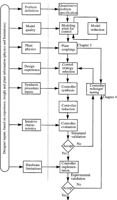
Figure 1.1 Dynamics, structures and control framework for analysis and design of flex-ible space structures. The thesis contributions to the framework are shaded.

Models (and design data) are shown in italics. . . . . 34

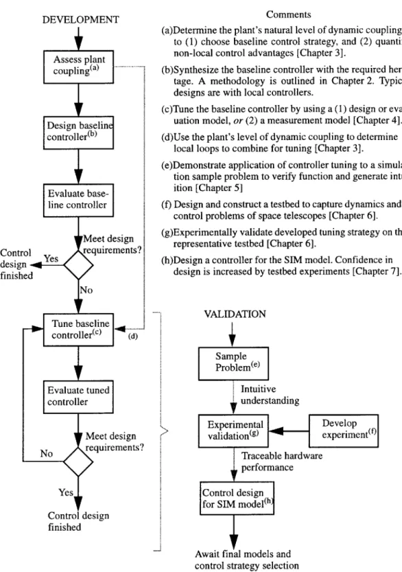
Figure 1.2 Figure 1.3 Figure 2.1 Figure 2.2 Figure 2.3 Controller synthesis and tuning . . . . 39

Thesis flow: the development and validation of global controller tuning for spaceborne telescopes . . . . 49

General control system interconnection . . . . 53

Standard feedback configuration . . . . 55

Small Gain Theorem block diagram . . . . 60

Figure 2.4 Divisive uncertainty . . . . 60

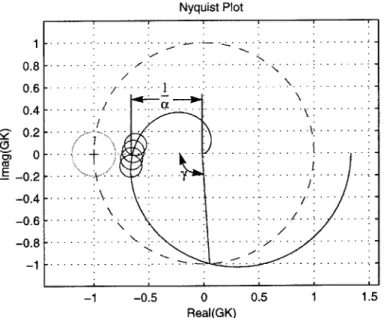
Figure 2.5 SISO Nyquist plot (positive frequency) is drawn with solid line. The unity gain circle is indicated with a dashed circle. The gain margin, a, and phase margin are, y, are indicted on the figure. Small circles along the locus corre-spond to balls of uncertainty at several respective frequency points. The cir-cle around the (-1,0) critical point indicated a guaranteed robustness region. . . . . 64

Figure 2.6 Controller design framework flowchart . . . . 68

Figure 2.7 Figure 3.1 Figure 3.2 Control implementation hardware. . . . . 73

Scaling the design model for control design . . . . 84

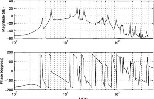
Channel transfer function of a balanced model. Phase is wrapped for plotting purposes. The 176 state balanced model (dashed) overlays the 270 state orig-inal model (solid). Without the numerically robust balancing technique the SIM model could not be balanced. . . . . 89

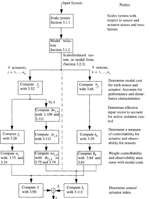
Figure 3.3 Simplified flow diagram of the sensor/actuator indexing algorithm. The manipulation of any rigid body modes is detailed in Section 3.2.3. . . 114

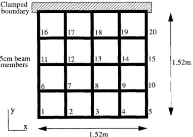
Figure 3.4 Test model for validating sensor/actuator indexing. Node locations for sen-sors and actuators are numbered. . . . 117

Figure 3.5 Complete enumeration of a reduced set of actuators and sensors for three control penalty/sensor noise settings. A unity white noise disturbance torque added at node 3 about the x axis. The performance is to minimize the RMS displacement of node 3. The sensor/actuator indexing algorithm choice is indicated by *. . . . 124

14 LIST OF FIGURES

Figure 3.6

Figure 4.1

Two mass/spring design example to demonstrate the application of the sen-sor/actuator assessment matrix for selecting sensor and actuators for the

LQG control problem. . . . 126

Two measures of stability robustness: The left plot corresponds to Ss where the shaded area measures the deviation of the maximum singular value of the Sensitivity over the 5 dB threshold. The right plot demonstrates Scr which measures the sum of the distances from the (- 1,0) critical point to the critical

Nyquist locus points marked with circles. . . . 134

Figure 4.2 Stability penalty term of Equation 4.8. Upper plot: Maximum s.v. of a Sensi-tivity Transfer Matrix. Bottom plot: stability penalty term plotted for three values of a. As a is increased the stability penalty for deviations greater than the 5 dB threshold is made sharper (i.e. small deviations are penalized like large deviations) . . . 137 Figure 4.3 Flow chart for an algorithm to compute the sensitivity of the maximum

sin-gular value of the Sensitivity transfer matrix with respect to controller parameters. Both design model and measurement model cases are

presented. . . . 144

Figure 4.4 Top: singular values of a sample sensitivity transfer matrix, Bottom: sensi-tivity of the singular values with respect to a controller parameter. Analytic and finite difference calculation is shown. . . . 146 Figure 4.5 _{Jordan (diagonal) form for an order n, MIMO system with n, inputs and nY}

outputs. . . . 160

Figure 4.6 Figure 4.7

Space of parameterized controllers, two parameter example . . . 172 Flow diagram of the tuning methodology including the iterative cost minimi-zation . . . 173

Figure 5.1 1-D Interferometer Sample Problem. Masses and springs are labeled. The

position of the masses is noted by xs where s is the mass' subscript. . . 182

Figure 5.2 The inertial force,fl.fd is a disturbance force passing through pre-whitening dynamics.fr is the rigid-body actuator. . . . 183 Figure 5.3 Magnitudes of transfer functions for the 1-D interferometer sample

problem . . . 185 Figure 5.4

Figure 5.5

A family of tuned controllers for the 1 -D interferometer sample problem:

starting with the classically-designed baseline controller, states are added and additional controls channels are added to result in a final tuned control-ler C4. Controlcontrol-lers are designed by tuning the previous controlcontrol-ler in the

dia-gram . . . 190 Performance and maximum s.v. of the Sensitivity (for

f>10

LIST OF FIGURES 15 Figure 5.6 Figure 5.7 Figure 5.8 Figure 5.9 Figure 5.10 Figure 5.11 Figure 5.12 Figure 5.13 Figure 5.14 Figure 5.15

Performance (top left), maximum and minimum singular values of the Sensi-tivity (bottom left) and MIMO Nichols plot (right) for baseline classical con-troller (solid) and a tuned concon-troller C4 (dashed). Open loop performance is indicated with a light solid line. . . . 192 Transfer function magnitudes for the baseline classical controller (solid) and C4 tuned controller (dashed). . . . ... . . . 193

A family of controllers designed to maintain performance as stability

robust-ness is improved. The left figure plots the maximum spike in the Sensitivity s.v. versus the stability robustness tuning parameter, P. The right figure plots the maximum s.v. of the Sensitivity as [3is increased (increasing

P

Multivariable Nyquist plot. The classical baseline controller is solid. The controller tuned to push the locus away from the critical point at frequencies greater than the VC mode (- 160 Hz) is dashed. . . . 197

Performance (top left), maximum and minimum singular values of the Sensi-tivity (bottom left) and MIMO Nichols plot (right) for baseline classical con-troller (dark) and a tuned concon-troller (dashed). The tuned concon-troller penalizes the distance from the critical point forf>150 Hz. Open loop performance is indicated with a light solid line. . . . 198 Performance (top left), maximum and minimum singular values of the Sensi-tivity (bottom left) and MIMO Nichols plot (right) for baseline classical con-troller (dark) and a tuned concon-troller (dashed). The tuned concon-troller penalizes the distance from the critical point for frequencies near the arm modes (i.e. Hz.). The arrow in the right plot indicates a shifting away from the critical point of the loop corresponding to the interferometer arm modes. Open loop performance is indicated with a light solid line. . . . 199

Nichols stability plots of the baseline (left) and tuned (right) case as damping of the symmetric and antisymmetric arm modes is varied. (= 1% is solid,

(=0.01% is dashed and (=0 is dash-dotted. The tuned controller is designed

to be more robust to uncertainty in the arm modes than the baseline control-ler by penalizing the distance from the critical point for frequencies near the arm modes (i.e.f~16 Hz) . . . 200 A family of tuned controllers for the 1-D interferometer sample problem:

starting with the baseline LQG controller, particular control channels are penalized and removed from the controller. Each controller is tuned from the previous controller in the diagram. . . . 202

Performance and maximum s.v. of the Sensitivity (for Hz) for the family of constrained-topology controllers of Figure 5.13. . . . 204 Performance (top left), maximum and minimum singular values of the Sensi-tivity (bottom left) and MIMO Nichols plot (right) for baseline classical

con-16 LIST OF FIGURES

troller (dark) and a tuned controller K4 (dashed). Open loop performance is

indicated with a light solid line. . . . 205

Figure 5.16 Transfer function magnitudes for the baseline LQG controller (solid) and K5 constrained-topology tuned controller (dashed). . . . 206

Figure 6.1 Space telescope / Origins Testbed control block diagram . . . 210

Figure 6.2 Origins Testbed . . . 213

Figure 6.3 Origins Testbed subsystems block diagram . . . 215

Figure 6.4 Origins Testbed: optical system block diagram . . . 217

Figure 6.5 Origins Testbed: optical system block diagram . . . 218

Figure 6.6 Optical delay line implementation . . . 218

Figure 6.7 Measured magnitudes for the Origins Testbed. A low frequency loop (band-width - 0.1 Hz) is closed from the encoder to gimbal to remove rigid-body drift during system identification. . . . 221

Figure 6.8 Autospectra of output measures during an observation. The disturbance is the average effect of the wheel imbalance as the wheel winds up to maintain accurate pointing. . . . 223

Figure 6.9 Measured (solid) and identified (dashed) disturbance to performance autospectra . . . 224

Figure 6.10 Block diagram of output analogous control . . . 228

Figure 6.11 Baseline slew controller structure . . . 230

Figure 6.12 Origins Testbed slew dynamics . . . 231

Figure 6.13 Baseline RWA slew controller, Kscw and encoder to RWA control loop gain, calculated with measured data. . . . 232

Figure 6.14 Gimbal momentum dump prefilter. Dashed: gimbal torque to RWA-to-ENC pointing with ENC-to-RWA loop closed, and solid: gimbal pre-filter magni-tude dynamics . . . 234

Figure 6.15 Measured slew control performance. Top: testbed pointing angle with refer-ence (dashed), Middle: gimbal action, Bottom: reaction wheel speed . 235 Figure 6.16 Baseline phasing controller structure. The loop indicated with the light line is closed in the SIM control strategy, but will not be closed in the simplified OT demonstration experiments. . . . 236

Figure 6.17 Baseline phasing controller for the voice coil actuator, K baseline con-troller for the piezo mirror actuator Kph,p, and the phasing loop gain . 238 Figure 6.18 Baseline fine-pointing controller and fine-pointing loop gain . . . 239

LIST OF FIGURES 17 Figure 6.19 Figure 6.20 Figure 6.21 Figure 6.22 Figure 6.23 Figure 6.24 Figure 6.25

Open-loop (solid) and closed-loop (dashed) performance of the baseline controller for the differential pathlength and fine pointing metrics as mea-sured by the laser interferometer (DPL) and the quad cell (QC) . . . . 240 Absolute stability and robustness of the baseline controller: simulated with data from the Origins Testbed, and experimentally measured (dashed) 242 Sensor Actuator Indexing in the presence of a controller . . . 242 OT tuned controller family: controllers are synthesized by tuning the previ-ous controller in the block diagram. . . . 246 Experimental performance autospectra: open-loop (light), baseline controller (solid), T 1l controller (dashed) . . . 248 Stability plots for T11 controller (solid) compared with a controller designed without the stability penalty, i.e. , (dashed) that achieves similar simulated performance. An expanded view new the critical point of the Nichols plot shows the dashed curve approaching dangerously close to the critical

point. . . . 249 Plots of performance and maximum Sensitivity s.v. for each of three incre-mental tuner controller designs from the controller family of Figure 6.22 (following arrows). RMS DPL and QC performance are listed with predicted and measured values. For the maximum Sensitivity s.v., progression along a path in Figure 6.22 is indicated with a progression towards a lighter curve. For presentation purposes not all maximum s.v. plots in the set of controllers are displayed. . . . 250

Figure 7.1 SIM Classic: one Possible design of the Space Interferometry Mission

spacecraft. (Graphic courtesy of JPL) . . . 254 Figure 7.2

Figure 7.3

Preparing the SIM model for control examples . . . 256 Subset of the magnitude of the transfer matrix for guide interferometer 1 of the SIM model. Attitude control loops are closed but the optics loops are

open. ... 261

Figure 7.4 Performance and stability of tuned fine-pointing controller. The top plot is the autospectrum of the external DPL of guide interferometer 1, the middle plot is the autospectrum of the differential wavefront tilt of guide

interferom-eter 2, and the lower plot are the maximum and minimum singular values of the Sensitivity transfer matrix. The open loop is plotted in dark solid and the baseline controller is dashed. . . . 266

Figure 7.5 SIM tuned controller family: controllers are synthesized by tuning the

previ-ous controller in the block diagram. . . . 267 Figure 7.6 Performance and stability of tuned phasing controller Si. The top plot is the

autospectrum of the external DPL of guide interferometer 1, the middle plot is the autospectrum of the differential wavefront tilt of guide interferometer 2, and the lower plot are the maximum and minimum singular values of the

18 LIST OF FIGURES

Sensitivity transfer matrix. The open loop is plotted in light solid, the base-line control case in dark solid and the tuned controller is dashed. . . . 269

Figure 7.7 Performance and stability of tuned fine-pointing controller S2. The top plot is the autospectrum of the external DPL of guide interferometer 1, the mid-dle plot is the autospectrum of the differential wavefront tilt of guide inter-ferometer 2, and the lower plot are the maximum and minimum singular values of the Sensitivity transfer matrix. The open loop is plotted in light solid, the tuned phasing control case is dark solid and the tuned controller is

dashed. ... ... 270

Figure 7.8 Performance and stability of final tuned controller S3. The top plot is the autospectrum of the external DPL of guide interferometer 1, the middle plot is the autospectrum of the differential wavefront tilt of guide interferometer 2, and the lower plot are the maximum and minimum singular values of the Sensitivity transfer matrix. The open loop is plotted in light solid, the base-line control case in dark solid and the tuned controller is dashed. . . . 271

Figure 7.9 Plots of performance and maximum Sensitivity s.v. for the incremental tuned controller designs from the controller family of Figure 7.5 (following arrows on the figure). RMS phasing and pointing performance are listed. . . 272

Figure 7.10 Figure 7.11 Figure A.1 Figure A.2 Figure A.3 Figure A.4 Figure A.5 Figure C. 1

Tuned and baseline phasing controller for guide interferometer 1. The base-line controller is light solid and the tuned controller is dashed . . . 273 Tuned and baseline fine-pointing controller for guide interferometer 1. The baseline controller is light solid and the tuned controller is dashed . . . 274 Recovering optimal estimates from local estimates . . . 303 Four spring design example to demonstrate a technique for selecting

reduced-order local models . . . 309 Hankel singular values for balanced full-order local models corresponding to each sensor . . . 310

Plot of normalized local estimator's global state estimate accuracies as the order of the local models is increased for proportional damping of (=0.001.

1 corresponds to global fully coupled estimation. The order (2,4,6,8) of the

local models increases as we ascend from light to dark. . . . 312 Plot of normalized local estimator's global state estimate accuracies as the order of the local models is increased for proportional damping of (-+ 1. 1 corresponds to global fully coupled estimation. The order (2,4,6,8) of the local models increases as we ascend from light to dark. . . . 313 Performance (top left), maximum singular value of the Sensitivity (bottom left) and Nichols plot (right) for the baseline LQG controller on the design model (solid) and measured data (dashed). The open loop is plotted with the light line in the performance plot. . . . 330

LIST OF FIGURES 19 Figure C.2 Figure D. 1 Figure D.2 Figure E. 1 Figure E.2 Figure E.3 Figure E.4 Figure E.5 Figure E.6 Figure E.7 Figure E.8 Figure E.9 Figure E.10 Figure E.11 Figure E.12 Figure E.13

Performance (top left), maximum singular value of the Sensitivity (bottom left) and Nichols plot (right) for the initial SWLQG controller (solid) and for the tuned SWLQG controller (dashed). Plots are generated with the

mea-sured plant data. The open loop is plotted with the light line in the perfor-m ance plot. . . . 331

Reaction wheel disturbance prefilter autospectrum. The disturbance increases as wheel speed squared and cuts off sharply at the highest wheel

speed frequency. . . . 335 Autospectra of the DPL and QC performance variables as the wheel winds-up during an observation. Measured data is indicated with the solid line, and

the estimated state-space model is indicated with the dashed line. The mod-eled spectra has the rough shape of the measured spectra. . . . 337 TI controller magnitudes (dashed), and baseline controller magnitudes (solid) . . . 340

Experimental performance autospectra: open-loop (light), baseline controller (solid), T1 controller (dashed) . . . 341 Stability plots for T1 controller: simulated control on design data (solid), and measured (dashed) . . . 341 T2 controller magnitudes (dashed), and TI controller magnitudes

(solid) . . . 342 Experimental performance autospectra: open-loop (light), TI (solid), T2 controller (dashed) . . . 343 Stability plots for T2 controller: simulated control on design data (solid), and measured (dashed) . . . 343

T3 controller magnitudes (dashed), and T2 magnitudes (solid) . . . 344

Experimental performance autospectra: open-loop (light), T2 (solid), T3 controller (dashed) . . . 345 Stability plots for T3 controller: simulated control on design data (solid), and measured (dashed) . . . 345 T4 controller magnitudes (dashed), and T3 controller magnitudes

(solid) . . . 346

Experimental performance autospectra: open-loop (light), T3 controller (solid), T4 controller (dashed) . . . 347 Stability plots for T4 controller: simulated control on design data (solid), and measured (dashed) . . . 347

T5 controller magnitudes (dashed), and T2 controller magnitudes

20 LIST OF FIGURES Figure E.14 Figure E.15 Figure E.16 Figure E.17 Figure E.18 Figure E.19 Figure E.20 Figure E.21 Figure E.22 Figure E.23 Figure E.24 Figure E.25 Figure E.26 Figure E.27 Figure E.28 Figure E.29 Figure E.30 Figure E.31

Experimental performance autospectra: open-loop (light), T2 controller (solid), T5 controller (dashed) . . . . . 349 Stability plots for T5 controller: simulated control on design data (solid), and measured (dashed) . . . 349

T6 controller magnitudes (dashed), and T5 controller magnitudes

(solid) . . . 350 Experimental performance autospectra: open-loop (light), T5 controller (solid), T6 controller (dashed) . . . 351 Stability plots for T6 controller: simulated control on design data (solid), and measured (dashed) . . . 351

T7 controller magnitudes (dashed), and T1 controller magnitudes

(solid) . . . 352 Experimental performance autospectra: open-loop (light), T 1 controller (solid), T7 controller (dashed) . . . 353 Stability plots for T7 controller: simulated control on design data (solid), and measured (dashed) . . . 353

T8 controller magnitudes (dashed), and T7 controller magnitudes

(solid) . . . 354 Experimental performance autospectra: open-loop (light), T7 controller

(solid), T8 controller (dashed) . . . 355 Stability plots for T8 controller: simulated control on design data (solid), and measured (dashed) . . . 355 T9 controller magnitudes (dashed), and baseline controller magnitudes

(solid) . . . 356 Experimental performance autospectra: open-loop (light), T8 controller

(solid), T9 controller (dashed) . . . 357 Stability plots for T9 controller: simulated control on design data (solid), and measured (dashed) . . . 357 T10 controller magnitudes (dashed), and T9 controller magnitudes

(solid) . . . 358 Experimental performance autospectra: open-loop (light), T9 controller (solid), T1O controller (dashed) . . . 359 Stability plots for T10 controller: simulated control on design data (solid), and measured (dashed) . . . 359

T11 controller magnitudes (dashed), and T10 controller magnitudes

LIST OF FIGURES 21

Figure E.32 Experimental performance autospectra: open-loop (light), T10 controller (solid), T 11 controller (dashed) . . . 361 Figure E.33 Stability plots for T11 controller: simulated control on design data (solid),

LIST OF TABLES

Research references for the dynamics, structures and controls

framework ... ... 36

Experimental test articles relevant to future spaceborne telescopes . . 46 Validation of developed techniques: test matrix . . . . 50

Variables to quantify a control problem . . . . 67

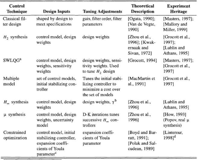
Non-exhaustive list of control strategies with (mostly) MIT SERC experi-m ental heritage . . . . 72

Inputs and outputs for sensor/actuator indexing algorithm . . . 115 Material properties of grid model, [Kim and Junkins, 1991]. . . . 117

Comparison of sensor/actuator indexing with simulated annealing and com-plete enumeration when the total flops is held constant. A unity white noise disturbance torque added at node 3 about the x axis. The performance is to minimize the RMS displacement of node 3. . . . 122

Comparison of sensor/actuator indexing with complete enumeration. Three disturbance/performance cases are tried, each at three levels of LQG con-trol. Each complete evaluation finds global optimum but requires 584 times more flops than the sensor/actuator indexing algorithm. . . . 125

Comparison of sensor/actuator indexing with simulated annealing. Three disturbance/performance cases are tried, each at three levels of LQG con-trol. The best of five 50 iteration simulated annealing runs is displayed for each case. Each simulated annealing solution requires 33 times more flops than the sensor / actuator indexing. . . . 126 System parameters and input/output signals for 2-dof sensor/actuator effec-tiveness assessment example . . . 127 Sensor/Actuator matrix, St, for 2-dof sensor/actuator effectiveness assess-ment. The channel deemed best is shaded. . . . 128

H2 cost for SISO LQG controllers designed for 2-dof sensor/actuator effec-tiveness assessment. The channel calculated to be best is shaded. . . . 128

Description of the terms of the augmented tuning cost. Included are refer-ences to the equations of the mathematical definitions of the cost compo-nents for both model-based and data-based tuning. . . . 132

Summary of the terms of the augmented cost function. The table lists expressions for the cost terms when either a state-space model is available,

24 LIST OF TABLES TABLE 5.1 TABLE 5.2 TABLE 5.3 TABLE 5.4 TABLE 5.5 TABLE 5.6 TABLE 5.7 TABLE 5.8 TABLE 5.9 TABLE 6.1 TABLE 6.2 TABLE 6.3 TABLE 6.4 TABLE 6.5 TABLE 6.6 TABLE 6.7 TABLE 6.8 TABLE 6.9 TABLE 6.10 TABLE 7.1 TABLE 7.2

or when measured data only is available. Designer thresholds and weights are all noted with an asterisk (*). . . . 158

Parameter values for the 1 -D Interferometer Sample Problem. . . . . 182

Structural modes of the 1-D interferometer model . . . 183 Input and output signals for the 1-D interferometer. Resolutions are

included for the sensors and actuators, intensities for the disturbances and requirements for the performances. . . . 184

Sensor/Actuator matrix, St, for 1-D Interferometer Model. Shaded blocks represent channels in used for a classically-designed local controller. . 186

Tuning terms (from Equation 5.2) for OT tuned controller family . . . 189

Performance and stability robustness of the family of controller of

Figure 5.4. . . . 191

Weights for the baseline LQG controller . . . 200 Tuning terms (from Equation 5.2) for OT tuned controller family . . . 202 Performance and stability robustness of the family of controller of

Figure 5.13. Both the fully connected and constrained topology (channels set to 0) controller cases are considered. . . . 203 Control requirements for space-based telescopes . . . 211

Origins Testbed actuator suite . . . 215

Origins Testbed sensor suite . . . 216

Signal definitions for the four-block control problem for the Origins Test-bed observation control. . . . 220

Sensor and Actuator indexing matrix for OT Model. . . . 226

Actuators and sensors for the Origins Testbed control examples . . . 227

Measured and predicted performance of baseline controller . . . 240 Modified Sensor and Actuator indexing matrix for the closed-loop, base-line-controlled OT Model . . . 243

Tuning terms (from Equation 6.14) for OT tuned controller family . . 245

OT tuned controller family: description and performance . . . 247 Signal definitions for the four-block control problem for the SIM observa-tion control. Resoluobserva-tions are included for the sensors and actuators, intensi-ties for the disturbances and requirements for the performances. . . . 257

Sensor and Actuator indexing matrix for the SIM model. Light shading cor-responds to phasing control channels. Dark shading corcor-responds to fine-pointing control channels. . . . 263

LIST OF TABLES 25 TABLE 7.3 TABLE 7.4 TABLE C.l TABLE C.2 TABLE E. I TABLE E.2 TABLE E.3 TABLE E.4 TABLE E.5 TABLE E.6 TABLE E.7 TABLE E.8 TABLE E.9 TABLE E.10 TABLE E.1 l

Tuning terms (from Equation 7.2) for SIM tuned controller family . . 267

Performance variables for the family of tuned SIM controllers. All absolute measures are RMS quantities. Decibel quantities are improvements of the controlled performance relative to the appropriate open-loop performance variable. . . . 268 Input and output signals for the MACE example . . . 329

Performance and stability robustness summary of the MACE controllers: Baseline LQG, Initial SWLQG and tuned SWLQG.

Measured and predicted performance of controller Ti Measured and predicted performance of controller T2 Measured and predicted performance of controller T3 Measured and predicted performance of controller T4 Measured and predicted performance of controller T5 Measured and predicted performance of controller T6 Measured and predicted performance of controller T7 Measured and predicted performance of controller T7 Measured and predicted performance of controller T9 Measured and predicted performance of controller T 10 Measured and predicted performance of controller Ti

. . . . 332 . . . 340 . . . 342 . . . 344 . . . 346 . . . 348 . . . 350 . . . 352 . . . 354 . . . 356 . . . 358 . . . 360

NOMENCLATURE

Abbreviations

BC baseline controller

CCD charge coupled device

dof degree of freedom

DPL differential pathlength

ENC encoder

FEM finite element method or finite element model

FSM fast-steering mirror

i/o input/output

JPL Jet Propulsion Laboratory

LQG linear quadratic Gaussian

LQR linear quadratic regulator

LTI linear time-invariant

MIMO multiple-input, multiple-output

MIT Massachusetts Institute of Technology

NGST Next Generation Space Telescope

ODL optical delay line

OT Origins Testbed

PZT mirror on piezo stack actuator

QC quad-cell photodiode

RB rigid body

RG rate gyroscope

RMS root mean square

RWA reaction wheel assembly

S/A sensor/actuator

SERC Space Engineering Research Center

SIM Space Interferometry Mission

SISO single-input single-output

ST star tracker

s.v. singular value

SVD singular value decomposition

SWLQG Sensitivity-Weighted Linear Quadratic Gaussian

VC Voice coil

28 NOMENCLATURE Symbols z y w x U A B, BU Cz Cy Dzw Dzu D,, D,, G(s) Gzw(s) Gzu(s) Gyw(s) GY (s) xc AC BC K(s) 0 S(s) A, B, Cs D, amax(-) GminG_) J(.) Kb(s) d(.) R Rz Ru R, q p performance variable sensor measurement

exogenous disturbances, including process and sensor noises plant state vector

actuator inputs

plant dynamics matrix

plant disturbance input matrix plant actuation input matrix

plant performance measurement matrix plant sensor measurement matrix

plant disturbance to performance feedthrough matrix plant actuation to performance feedthrough matrix plant disturbance to sensor feedthrough matrix plant actuation to sensor feedthrough matrix plant transfer matrix

plant disturbance to performance transfer matrix plant actuator to performance transfer matrix plant disturbance to sensor transfer matrix plant actuator to sensor transfer matrix

controller state variable controller dynamics matrix controller input matrix controller output matrix controller transfer matrix frequency (radian/second) Sensitivity transfer matrix Sensitivity dynamics matrix Sensitivity input matrix Sensitivity output matrix Sensitivity feedthrough matrix maximum singular value operator minimum singular value operator

maximum singular value over all frequency (H. norm) cost function

baseline controller transfer matrix

distance function for comparing controllers resolution-based scale factor for the sensors

performance-requirement-based scale factor for the performance variables resolution-based scale factor for the actuators

intensity-based scale factor for the disturbances left eigenvector of A

NOMENCLATURE 29

f

h observability measure

J cost or modal control cost

V modal output state cost

a performance-weighted controllability measure

disturbance-weighted observability measure

Be output-isolation effective actuator input matrix

JA augmented tuning cost

M penalty term for control use

SR penalty term for stability non-robustness

Ss penalty term for deviations of max s.v. of Sensitivity greater than threshold

Scr penalty term for distance of Nyquist locus to the critical point

Ycr stability non-robustness term mixing parameter

p stepsize

Chapter 1

INTRODUCTION

Strict requirements on the performance of future space-based observatories such as the Space Interferometry Mission (SIM) and the Next Generation Space Telescope (NGST), will extend the state-of-the-art of mission-critical spaceflight-proven active control design. A control design strategy which combines the high performance and stability robustness guarantees of modem, robust-control design with the spaceflight heritage of conventional control design is proposed which will meet the strict requirements, while maintaining traceability to the successful controllers from predecessor spacecraft.

The thesis outlines a technique for tuning baseline controllers to meet strict requirements while maintaining the heritage to previous missions. Two principal tools are developed: an analysis algorithm that quantifies each sensor/actuator combination's effectiveness for control, and a design engine which tunes a baseline controller to improve performance and/or stability robustness. The designer makes use of the sensor/actuator indexing tool to select which control channels to emphasize in the tuning. The tuning tool is flexible and allows the alteration of the controller topology, trades of performance and stability robust-ness, and limits of the deviation of the tuned controller from the heritage-rich baseline controller. Further, the tuning algorithm can operate with the plant's design model or directly with the plant's measured frequency response data.

The use of the tuning technique will be placed in context with a high-level control design methodology. The sensor / actuator indexing tool and the tuning technique will be

32 INTRODUCTION

ated on a sample problem, and then demonstrated on a laboratory test article with similar dynamics, a similar sensor suite, and a similar actuator suite to future space-based obser-vatories. The development of the test article, the first to combine large-angle slewing with nanometer optical phasing in the presence of spacecraft-like disturbances, is a contribution of the thesis and will be presented in suitable detail. Lastly the tools will be applied to a model of the SIM spacecraft.

The introduction is divided into a summary of the research objectives, a placement of the work in the context of other dynamics and control research for space-borne telescopes, a

review of relevant previous work, and a roadmap of the thesis.

1.1 Research Objectives

The fundamental goal of the research is to improve the control technology readiness for spaceborne telescopes. The work is motivated by three characteristics of future space-based telescopes:

1. No 1-g deployment: Future spaceborne telescopes are large in dimension and

lightweight and will not be able to support their own weight in a gravity field. No ground testing or model updating will be possible. The initial con-troller must be designed with sufficient stability robustness using a non-updated finite element method (FEM) model. Further, the controller may require updating to handle inevitable on-orbit model/plant mismatches. 2. Tight performance requirement: The pointing and phasing requirements are

beyond the current state-of-the-art. To improve performance, the controller should take advantage of all relevant sensor / actuator control channels and of knowledge of disturbance statistics.

3. Mission profile: Future spaceborne telescopes are expensive and have a high

public profile. Instability and failure are not acceptable. A control strategy with spaceflight and experimental heritage should be employed.

We wish to begin to bridge the gap between classical design with spaceflight heritage and modern optimization-based design, with the hope to improve the achievable control per-formance so that the tight imaging requirements can be met while maintaining the required stability robustness. The theory/practice gap is addressed in [Bernstein, 1999] for

Research Objectives 33

general control theory. The work in this thesis attempts to link theory and practice for flex-ible spacecraft control.

Particular objectives of this research can be summarized as:

- Outline a framework for the design of controllers for lightweight flexible spacecraft.

- Develop a technique to quantify the suitability of a plant for local control, and to quantify the advantages of global control. In particular we wish to

- Quantify the effectiveness of sensors and actuators for control,

- Determine the incremental effect of adding sensors and actuators.

. Develop a control design technique which takes advantage of modem opti-mal control theory while preserving the critical mission heritage of conven-tional, classical control designs. We adopt a strategy of tuning a baseline controller (with mission critical heritage). The desirable features of the methodology include:

- improvements in performance and/or stability robustness over the baseline controller,

- an ability to control the deviation of the tuned controller from the baseline controller,

- an ability to tune control designs using design models and experimentally determined measurement models,

- an ability to quantify and take advantage of the addition of extra states to the baseline controller,

- an ability to quantify and take advantage of the enhancement of coupling in the baseline controller.

- Develop a laboratory test article which captures the relevant dynamics and control issues anticipated for future based lightweight, flexible space-craft.

- Experimentally validate the control design methodology on the laboratory test article. We follow a procedure anticipated for the control design of the Space Interferometry Mission: first, design and implement a baseline con-troller with conventional, classical techniques, and then apply the developed methodology to arrive at a tuned, final design.

- Demonstrate the application of the control design methodology to an exist-ing integrated model of the Space Interferometry Mission. We begin with the JPL/MIT-designed baseline controller, synthesized with conventional,

classi-34 INTRODUCTION

cal techniques, and then apply the developed methodology to arrive at a tuned, final design.

1.2 Research Context

The control design for complex space structures must be placed within the context of the entire system design [Joshi, 1999]. The MIT Space Systems Laboratory has developed a framework for the analysis and design of the structure, dynamics and control for future spaceborne telescopes. The framework provides a structured environment for the model-ing, model assembly and conditionmodel-ing, analysis, evaluation against requirements, and if necessary, redesign for flexible space structures. Application of the framework to NGST is presented in [de Weck et al., 2000]. Figure 1.1 is a framework block diagram.

MODELING MODEL BASELINE CONTROL DESIGN

PREPARATION AND ANALYSIS

Exit if the

Uncer-

Uncer-tainty i tainty

database Ianalysis

Figure 1.1 Dynamics, structures and control framework for analysis and design of flexible space struc-tures. The thesis contributions to the framework are shaded. Models (and design data) are shown in italics.

Literature Review 35

The four column headings in the framework correspond to integrated modeling steps, while the individual blocks correspond to step components (tools where applicable). The framework is entered with an initial design. The design is modeled, and the FEM

state-space physics-based model is assembled from the avionics, disturbance, and structural

models. The model is conditioned and if a prototype is available measured data is used for model updating. Alternately system identification can be used to estimate a state-space

measurement model from the measured data. With a state-space model a tool developed in

Chapter 3 can be used to assess the effectiveness of particular sensors and actuators for control. The sensor/actuator effectiveness assessment along with a state-space plant model (or measured design data) are used to design a baseline controller. The baseline controller, sensor/actuator assessment, plant model (physics-based, measurement, or direct data), and the result of an uncertainty analysis (to set stability margins requirements) feed the con-troller tuning methodology of Chapter 4. The resulting concon-troller improves the perfor-mance and/or stability robustness of the baseline controller without losing the spaceflight heritage of the baseline controller. By appending the controller to the physics-based model we can assess the effect of disturbances, performance and sensitivity of the system. The sensitivity analysis allows an isoperformance trade of the subsystem requirements, leading to a (if necessary) plant redesign. Table 1.1 references the MIT research contributions that make up the framework.

The tools developed in this thesis provide critical contributions to the dynamics, structures and control framework for analysis and design future spaceborne telescopes.

1.3 Literature Review

Control design for lightweight flexible space structures and the control-structure interac-tion is an area which has received much atteninterac-tion in the literature. [Crawley et al., 2001] provides an overview of the dynamics and control of lightly damped structures. The appli-cation and implementation of lightweight flexible space structure control was demon-strated on-orbit with success during the Middeck Active Control Experiment (MACE)

36 INTRODUCTION

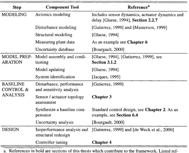
TABLE 1.1 Research references for the dynamics, structures and controls framework

Component Tool Avionics modeling

Disturbance modeling Structural modeling Measuring plant data Uncertainty database Model assembly and condi-tioning

Model updating System identification

Referencea

Includes sensor dynamics, actuator dynamics and delay [Glaese, 1994], Section 2.2.7

[Gutierrez, 1999] and [Masterson, 1999] [Glaese, 1994]

As an example see Chapter 6 [Bourgault, 2000]

[Glaese, 1994], [Gutierrez, 1999], see

Section 3.1.2

[Glaese, 1994] [Jacques, 1995]

BASELINE Disturbance, performance [Gutierrez, 1999] CONTROL & and sensitivity analysis

ANALYSIS Sensor / actuator topology _{Chapter 3} assessment

Synthesize a baseline com- Standard control design, see Chapter 2. As an pensator example, see Section 6.4

Uncertainty analysis [Bourgault, 2000]

DESIGN Isoperformance analysis and [Gutierrez, 1999] and [de Weck et al., 2000] structural redesign

Controller tuning Chapter 4

a. References in bold are sections of this thesis which contribute to the framework. Listed ref-erences are representative and are not meant to be exhaustive. Refref-erences are principally current and legacy research from the MIT Space Systems Laboratory which led to the devel-opment of the framework.

program [Miller et al., 1996]. However, the techniques with the greatest performance were modem model-based control designs which have little on-orbit heritage in non-experi-mental applications. A tuning strategy is adopted to link modem robust optimization tech-niques to conventional spacecraft control techtech-niques.

An important component of the work is an algorithm to assess the suitability of sensor and actuator combinations for control. Based on the sensor/actuator assessment, the designer can select control channels to emphasize when applying the tuning methodology. We review techniques to determine the suitability of actuators and sensors for control design

Step MODELING

MODEL PREP-ARATION

Literature Review 37

and find that a technique which incorporates knowledge of the disturbance and perfor-mance to index sensors/actuator combinations for control is needed.

We review controller tuning and find that an optimization-based frequency-domain strat-egy is lacking with the following critical characteristics: (1) tunes a general baseline con-troller, (2) allows specification of the topology (order and sensor / actuator connectivity) of the tuned controller parameters (3) designs with an explicit metric of stability robust-ness, (4) allows specification of the tuned controller's deviation from the baseline control-ler, and (5) tunes with a design-model and/or measured-data.

Further, we review spacecraft-like controlled structure laboratory testbeds and demon-strate that a testbed which captures all elements of the operation of a space-based observa-tory: slewing, phasing, pointing, and optical capture in the presence of realistic disturbances, has not been previously developed.

1.3.1 Sensor / Actuator Assessment for Control Effectiveness

Most relevant research in the literature for assessing sensor/actuator control effectiveness is in the area of actuator and sensor placement for the control problem. [Anderson, 1993] includes a detailed literature survey on the actuator placement problem for structural sys-tems.

Closed-loop sensor / actuator assessment

Closed-loop techniques, whereby a constrained topology controller is synthesized and evaluated, are expected to provide the most direct and accurate comparisons of sensor/ actuator topologies. [Mercadal, 1991] provides H2 optimal first-order necessary

condi-tions for block diagonal controller topologies. In practice though, the constrained topology

H2 optimal controllers prove difficult to synthesize. Recently [Hassibi et al., 1999]

devel-oped a structural controller design technique which can be used to derive a sparse low-authority controller based on a relaxed linear programming constraint. The sensor/actuator topology is not pre-specified but determined simultaneous with the control design. The

38 INTRODUCTION

technique is extended to linear perturbations of the high-authority (performance improv-ing) control, but does not rank the effectiveness of the sensors and actuators. The closed-loop sensor evaluation problem is examined in [Mallory and Miller, 2000] where the abil-ity of each sensor to H2 optimally estimate each of the system states is determined by a

solution of a Ricatti Equation. The technique can be extended to the dual, actuator prob-lem, but combining the sensor and actuator problems is difficult.

Open-loop sensor/actuator assessment

In open-loop techniques, the design model is analyzed without explicitly solving for the controller. One set of strategies for the actuator/sensor placement problem involve defin-ing a measure of controllability and observability and selectdefin-ing sensor/actuator combina-tions with the highest combined observability/controllability [Gawronski and Lim, 1996], [Lim, 1992]. [McCasland, 1989] is similar but includes weightings by fault probabilities. To eliminate the difficulty of discrete locations, [Maghami and Joshi, 1993] approximate sensor measurements and actuator forces with spatially continuous functions to arrive at a well-posed nonlinear programming problem. These approaches use the actuator-to-sensor transfer matrix and do not exploit knowledge of the disturbance and performance charac-teristics.

Skelton's modal cost analysis [Skelton and Hughes, 1980] breaks up the system's H2

per-formance cost into a sum of modal contributions. By examining the effect of each actua-tor, and the measure of each sensor on modes of the open-loop cost, a subset of sensors or actuators can be chosen which are determined to be effective [Skelton and Chiu, 1983], [Lin, 1996]. The simultaneous selection of sensors and actuators is not presented. The technique is modified to account for closed-loop effects in [Skelton and DeLorenzo, 1983] whereby the LQG problem is solved, sensors and actuators with little contribution are removed and the process is repeated. What results is a subset of actuators and sensors that are suited for LQG control. The technique does not index actuators and sensors for a gen-eral control topology.