Estimating marine icing on offshore structures using RIGICE04

Publisher’s version / Version de l'éditeur:

Vous avez des questions? Nous pouvons vous aider. Pour communiquer directement avec un auteur, consultez la première page de la revue dans laquelle son article a été publié afin de trouver ses coordonnées. Si vous n’arrivez pas à les repérer, communiquez avec nous à PublicationsArchive-ArchivesPublications@nrc-cnrc.gc.ca. Questions? Contact the NRC Publications Archive team at

PublicationsArchive-ArchivesPublications@nrc-cnrc.gc.ca. If you wish to email the authors directly, please see the first page of the publication for their contact information.

https://publications-cnrc.canada.ca/fra/droits

L’accès à ce site Web et l’utilisation de son contenu sont assujettis aux conditions présentées dans le site LISEZ CES CONDITIONS ATTENTIVEMENT AVANT D’UTILISER CE SITE WEB.

11th International Workshop on Atmospheric Icing of Structures [Proceedings],

2005

READ THESE TERMS AND CONDITIONS CAREFULLY BEFORE USING THIS WEBSITE.

https://nrc-publications.canada.ca/eng/copyright

NRC Publications Archive Record / Notice des Archives des publications du CNRC : https://nrc-publications.canada.ca/eng/view/object/?id=e5e4d5ee-d0fa-472b-ae39-52842f307c7a https://publications-cnrc.canada.ca/fra/voir/objet/?id=e5e4d5ee-d0fa-472b-ae39-52842f307c7a

NRC Publications Archive

Archives des publications du CNRC

This publication could be one of several versions: author’s original, accepted manuscript or the publisher’s version. / La version de cette publication peut être l’une des suivantes : la version prépublication de l’auteur, la version acceptée du manuscrit ou la version de l’éditeur.

Access and use of this website and the material on it are subject to the Terms and Conditions set forth at

Estimating marine icing on offshore structures using RIGICE04

Dr. T.W. Forest, Dr. E.P. Lozowski, and Dr. Robert Gagnon

Dept. of Mechanical Engineering*, Dept. of Earth and Atmospheric Sciences*, and NRC – Institute for Ocean Technology, St. John’s NF

*University of Alberta, Edmonton, Alberta, Canada, T6G 2G8, tom.forest@ualberta.ca

Estimating Marine Icing on Offshore Structures

using RIGICE04

Abstract— A program for simulating ice accretion on an

offshore structure due to spray generation from wave-structure impacts is presented in this paper. The program is an upgraded version of RIGICE that was first developed in 1987 and incorporates a number of improvements, specifically: a more accurate expression for the equilibrium freezing point of seawater, an empirical expression for sponginess of marine ice as a function of air temperature, a spray liquid water content versus height model that is matched with field data, and a new algorithm for estimating the frequency of significant spray events that generate spray clouds above 10 m high. Comparisons of ice accretion predictions are presented between the current version, RIGICE04 and a previous version, N_RIGICE. Generally, RIGICE04 predicts lower total ice accretion mass than N_RIGICE. RIGICE04 results are also compared with measured ice accretion duration on an offshore rig operating on the East coast of Canada. The current prediction is in good agreement with the measured duration; while the N_RIGICE prediction was more than twice the measured duration. RIGICE04 is more accurate than N_RIGICE although more comparisons with field data are required.

I. INTRODUCTION

CE accretion on offshore structures is a problem that must be considered by rig designers, rig operators, and regulatory agencies. For ground-based structures, the problem relates to increased cross-sectional area of the support members with a consequent increase in lateral forces generated by wave-structure interactions. For semi-submersible rigs, there is the added concern of increased dead weight due to accreted ice resulting in reduced freeboard or reduced deck load.

A computer program called RIGICE was developed in 1987 [1], [2] to determine icing norms and extremes for offshore structures located in Canadian waters. It was intended to be a program that could be run quickly and contained several simplifications of existing models, namely the Norwegian icing model, ICEMOD originally developed in 1986 and modified in 1988 [3]. Since then RIGICE has undergone modifications to some of the algorithms, particularly those dealing with spray generation due to wave-structure impact. The specific objectives of this project were:

1. To upgrade the code with new icing algorithms 2. To make the code accessible to all interested parties 3. To compare predicted ice loads with previous

predictions using RIGICE.

In Section II, modifications that were made to the icing algorithms in RIGICE are reviewed particularly the one dealing with spray generation due to wave-structure interaction. Section III describes the results of a comparison of RIGICE04 simulations with previous simulations obtained using a modified version of the original code, N_RIGICE. The N_RIGICE simulations were presented by Lozowski et al. [4].

II. ICING ALGORITHMS

There were several areas in which the N_RIGICE model was upgraded. Broadly speaking, these fell into two categories: spray generation and properties of the accreted ice. A. Spray Generation

The spraying data obtained on Tarsiut Island [5] are used to estimate the spraying frequency and develop a new liquid water content equation for the spray cloud. Although these data were measured on an artificial island and not on an offshore rig, it was found that the new liquid water content equation produces a more realistic spray flux for rigs than other liquid water content equations in the literature.

1. Estimating the Spraying Frequency:

The cumulative probability distribution, P that a wave will exceed height H is given by Blevins [6]

P H H H ( ) exp( ) / = −2 2 1 3 2 (1)

where H1/3 is the significant wave height (m). Spraying experiments performed on Tarsiut Island from August 20-21, 1982 [5] showed that, on average, there were 24 large spray clouds per hour (~10 m high), that produced significant spraying of the island. During the observation period, the wind speed was 16.6 ms-1 from the northwest, with a significant wave height of 2.5 m. Using the equations of Bretschneider [7] and Lighthill [8], one may deduce that there was a total of 576 waves impacts per hour. Of these 576 waves, only 24 of them produced large spray clouds (~10 m high). Hence, given the above meteorological and oceanographic conditions, the critical wave height, Hc that gave rise to the 24 large spray clouds can be directly calculated from (1): P H H H c c ( ) exp( ) / = −2 = 24 576 2 1 3 2 (2)

I

This yields a critical wave height, Hc of 3.15 m as the minimum wave height needed to produce a “large” spray cloud. Now, for a general significant wave height, the probability that any one wave will exceed the critical wave height is: 19.85 ( 3.15) exp( ) 2 1/ 3 P Hc H ≥ = − (3)

From wind speed and fetch, the number of waves, Nwave produced per hour can be calculated from Bretschneider [7] and Lighthill [6]. Then, multiplying Nwave by P(Hc=3.15), the number of “large” sprays generated per hour, Nspray may be determined, and thence the duration for one “large” spray cycle. It is not obvious that the “large” spray cloud observations made on an artificial island such as Tarsiut, are immediately transferable to an offshore rig in this way. Once full-scale or model scale data for a rig are available, this approach should be reviewed.

2. Spray Cloud Liquid Water Content:

Based on the work of Borisenkov et al. [9], Makkonen and Lozowski [10], Horjen and Vefsnmo [11], and Brown and Roebber [12], the liquid water content, LWC or mass per unit volume of a wave-collision-generated spray cloud may be expressed as a function of height as follows:

LWC z( )=K H_{1 1 3}2_/ exp(−K z)

2 (4)

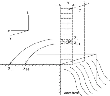
where K1 and K2 are empirical constants, and z is height above the top of the wave-wash zone. The fact that (4), in principle, describes a cloud of infinite height is of little practical consequence, since the liquid water content typically drops off sufficiently rapidly with height that there is virtually no spray beyond several scale heights. Let us consider a spray cloud with base dimensions of lx and ly (Fig.1). Then the total water z z x x

l

l

Fig. 1. Schematic diagram of a spray cloud generated by a wave-structure impact.

mass, Mz in the entire spray cloud can be calculated by integrating (4) from 0 to infinity:

M K K H l l z = ( ) 1 2 1/ 3 2 x y x (5) During the August 20-21 spraying experiments [5], spray water was collected in buckets set out on the island surface perpendicular to the sea wall. The mean horizontal spraying flux density data, m’, for a single spray, was found to fit the following equation:

' 6.904 exp( 0.217 )

m = − (6) where x is the distance from the sea wall (m) and m’ has units of kg m-2. It should be noted that the spray flux density is assumed to be a function of x only. The total spray mass, Mx which impinges along a horizontal spray zone perpendicular to the sea wall may be calculated by integrating (6) from 0 to infinity. The result is Mx = 31.82ly kg per spray. Conservation of spray mass requires that the total spray mass in the initial cloud must equal the total impinging spray mass on the surface of the island, hence Mx = Mz. Therefore,

K K l_x 1 2 5 09 = . (7) Substituting (7) into (4), the liquid water content equation becomes: LWC z K l_x H K ( )= . / exp( ) 5 09 2 1 3 2 2z − (8) We can once again use the Tarsiut Island data in order to estimate K2 using the following procedure. Let us consider a vertical segment of a spray cloud with dimension zI – zI-1, lx and ly as shown in Fig.1. The mass of spray in this segment is transported by the wind and gravity onto the surface and impinges over the distance xI-1 to xI. Then, from (6), the mean horizontal spray density between xI-1 and xI (m'(xI-1,xI)) may be written: m x x x x x x I I I I I I '( , ) . ( )(exp( . ) exp( . )) − − − = − − − − 1 1 1 318164 0 217 0 217 (9)

The average liquid water content (LWC z( I−1,zI)) inside the segment from zI-1 to zI can be determined from (8) to be:

LWC z z l z z H K z K I I x I I I I ( , ) . ( ) (exp( ) exp( )) − − − = − − − − 1 1 1/3 2 2 1 2 5 09 z (10)

When this segment of spray is carried onto the ground by the winds and gravity, the average spray density on the surface between xI-1 and xI (c x'( I−1,xI)) becomes:

c xI xI LWC zI zI v I v I T z z sp '( ₋₁, )= ( ₋₁, )( ( )+ ( −1)) 2 (11) where

vz(I): vertical velocity of spray droplets at a distance xI from the sea wall (ms-1).

vz(I-1): vertical velocity of spray droplets at a distance xI-1 from the sea wall (ms-1).

Tsp: spray duration for a single spray cloud (s). For a single spray cloud, the spray duration is given by:

T l v I v I sp x x x = + − 2 1 ( ) ( ) (12) where

vx(I): horizontal velocity of spray droplets at a distance xI from the sea wall (ms-1).

vx(I-1): horizontal velocity of spray droplets at a distance xI-1 from the sea wall (ms-1).

The droplet velocity vector was determined using a drop trajectory model. Using (9) to (12), an optimized value of K2 was then determined by minimizing the difference between the measured [5] and computed mean horizontal spray densities (m'(xI-1,xI)) and (c x'( I−1,xI)). The optimized value of K2 is 0.53. It should be noted that the length of the spray cloud, lx , affects only the spray period, and not the amount of spray received. Consequently, we assume a value of 2 m for lx which is probably close to the horizontal thickness of a typical spray cloud. Hence K1 is 1.35. Finally, the liquid water content equation becomes:

LWC z( )=1 35. H1 3/ exp(−0 53. z)

2

(13) It should be noted that (13) gives the liquid water content for one single spray with units of kg m-3 . It should be kept in mind that (13) has been derived from spraying data from one site only and more field data is required to refine this result. 3. Other LWC Equations:

There are several other spray cloud LWC relations in the literature. The most commonly used are listed below. In each case, the units of liquid water content are kg m-3.

a. Horjen and Vefsnmo [11]:

) 2 exp( 1 . 0 H H z w= − (14) where w is the time-averaged spray cloud liquid water content, H is the wave height (m) and z (m) the elevation above mean sea level.

b. Brown and Roebber [12]: ) ) 2 ( exp( 6 . 4 2 s H z w= − (15) where Hs is the root-mean-square wave height (m).

c. Zakrzewski [13]: ) 55 . 0 exp( 2 z HV w w= o r − (16) where wo = 6.1457 x 10-5 and Vr is the ship speed relative to an oncoming wave (ms-1).

d. Makkonen and Lozowski [10]:

) 55 . 0 exp( 5 . 2 _z H w w= o − (17) where wo = 1.3715 x 10-3. It should be noted that the liquid water content, w, in (14) to (17) is a time-averaged value, over the duration of the spray cycle, while the liquid water content in (13) represents the value for a single spray cloud. Incorporating the liquid water contents given by (13) to (17) into RIGICE04 would require averaging the spray generation over the entire spray period; this was not done in the present study.

4. Comparison with Observations:

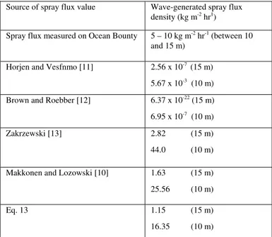
The semi-submersible drilling platform, OCEAN BOUNTY, which operated in Lower Cook Inlet near Kamishak Bay during the Winter of 1979/1980, experienced several icing events. In the most severe event, an estimated 500 tons of ice accumulated on the platform. The spray flux required at deck level (10-15 m above MSL) to produce icing of that severity is estimated to be 5 to 10 kg m-2 hr-1 [1]. During the period of the icing event, the average wind speed was 45 ms-1 from 290º to 300º, and the mean significant wave height was 3.8 m. Table 1 shows the results of spray flux computations using (13) to (17).

Table 1. Estimated spray flux density at deck level on theOcean

Bounty from (13) to (17).

It can be seen from Table 1 that spray fluxes vary greatly and this reflects the fact they were developed for various climatic factors and spray generation mechanisms. However, the spray flux densities computed using (16), (17), and (13) are comparable with observations on the OCEAN BOUNTY. Since (13) is closest to the observations and since it is tuned using real spray flux data, albeit on Tarsuit Island, we have incorporated it into the revised RIGICE model.

B. Accreted Ice Properties

A number of modifications were made to the algorithms dealing with the accreted ice mass: equilibrium freezing point of brine, and sponginess (liquid fraction) of accreted ice.

Source of spray flux value Wave-generated spray flux density (kg m-2 _hr1₎

Spray flux measured on Ocean Bounty 5 – 10 kg m-2 _hr-1 _{(between 10}

and 15 m) Horjen and Vesfnmo [11] 2.56 x 10-7 _{(15 m)}

5.67 x 10-3 _{(10 m)}

Brown and Roebber [12] 6.37 x 10-22 _{(15 m)}

6.95 x 10-7 _{(10 m)}

Zakrzewski [13] 2.82 (15 m) 44.0 (10 m) Makkonen and Lozowski [10] 1.63 (15 m) 25.56 (10 m) Eq. 13 1.15 (15 m) 16.35 (10 m)

1. Freezing Point of Brine:

Based on the work of Assur [14], we have derived a more accurate relation between brine salinity, Sb and its corresponding equilibrium freezing temperature, Tf for three temperature regimes. The equations are listed below:

1st regime T S S f b b = − − 54 1126 1 . ( ) (18)

for –7.7 ºC ≤ Tf ≤ 0 °C and 0 ≤ Sb ≤ 124.7 o/oo. Note that Sb is expressed as a decimal fraction when inserted in (18), (19), and (20). 2nd regime T S S f b b = − − 0 063 1 063 0 01031 1 . . . ( ) (19)

for -23 °C ≤ Tf < -7.7 °C and 124.7 < Sb ≤ 230.8 o/oo 3rd regime S x T T x T T b f f f f = + + + + − − 3 3136 10 0 01524 0 4752 3 3136 10 0 01524 1 4752 4 2 4 2 . . . . . . (20)

for -36 °C ≤ Tf < -23 °C and 230.8 < Sb ≤ 262.5 o/oo. 2. Ice Accretion Sponginess:

Unfrozen brine trapped within accreted ice can account for up to 50% or more of the accreted ice load. Hence it is important to account for it accurately. To this end, we have made use of the experimental data acquired by Shi and Lozowski [15] in the Marine Icing Wind Tunnel at the University of Alberta. They determined relations between ice accretion sponginess (both fresh and saline) and environmental conditions such as air temperature, Ta , wind speed, spray flux and spray droplet temperature. Although sponginess depends on all of these parameters, a preliminary analysis of the experimental data suggests a very simple parameterization, namely, that sponginess is approximately constant with a value of 0.4 (liquid fraction) at air temperatures between –5 °C and -25ºC. At air temperatures warmer than –5 °C, the sponginess decreases linearly with increasing air temperature and reaches zero at the equilibrium freezing temperature. This can be expressed in equation form as follows, with sponginess,

λ

λ = 40 (21)

for Ta ≤ -5 ºC;

λ= −12 6422. T_a−23 211. (22)

for -5 ºC < Ta ≤ 1.836 ºC .

It should be noted that (21) and (22) are not universal. They are based on an assumed spray salinity of 35 o/oo. Moreover, at very low temperatures, the sponginess can drop below 40 % when there is no water shed from the icing surface.

III. COMPARISONOFRIGICE04ANDN_RIGICE A modified version, N_RIGICE of the original icing code was used in the simulations presented in [4]. The new icing algorithms were incorporated into the current version, RIGICE04 and was coded as an Excel spreadsheet. The icing algorithms were imbedded in the spreadsheet as Visual Basic subroutines. The advantage of RIGICE04 is its ease of use compared to N_RIGICE which was coded in Fortran.

In this section, we present a set of ice accretion simulations that were conducted using the revised RIGICE04 spreadsheet in order to compare with results using the N_RIGICE version. The original code that was used to simulate ice accretion on the SEDCO 709 offshore rig was N_RIGICE and the simulations were presented in the report by Lozowski et al. [4] for the winter seasons from 1992 to 2000 although only the last two winter seasons are discussed below. The meteorological data that was used in these simulations was collected on the Rowan-Gorilla III operating at 43.8ΕN and 60.6ΕW, about 75 km southwest of Sable Island off the coast of Nova Scotia, Canada.

A total of 31 potential icing events (PIE’s) were identified in the two winter seasons spanning 1998 to 2000 for the original ice accretion simulations. In the following discussion we use the same PIE numbering system as defined in [4]. For the 1998-1999 there were 17 PIE’s and for the 1999-2000 season there were 14 PIE’s. The original meteorological data included only date and time, air temperature, wind speed, and wind direction. The input meteorological data file requires additional information including dew point, atmospheric pressure, sea surface temperature, significant wave height, significant wave period, and seawater salinity. The simulations use the following default values which were kept constant throughout each PIE: dew point temperature corresponding to a relative humidity of 84%, atmospheric pressure of 1013.3 mbar, and sea surface salinity of 35‰. The sea surface temperature was varied for each month based on estimates obtained from the U.S. Navy Marine Grid Point Database CD for the grid point location at 44ΕN and 61ΕW. The significant wave height and period were calculated using the fetch-dominated limit of the Bretschneider equation [16] with fetch equal to 185.4 km (100 nautical miles). These are the same values that were used in the original simulations using N_RIGICE.

The following criteria are used to define a PIE [17]:

1. A PIE begins when the air temperature falls below the equilibrium freezing point of seawater (-1.96 ΕC for a salinity of 35 o/oo) and the wind speed exceeds 0 m/s.

2. A PIE ends when either the air temperature rises above the freezing point for at least 12 consecutive hours or the wind speed drops to 0 m/s for at least 12 consecutive hours. If the criteria for a PIE are satisfied again after a lapse of less than 12 consecutive hours, it is assumed that the previous PIE has simply continued following a brief pause. No account is taken of potential melting or shedding of the accreted ice during such short intervals. Should the criteria for a PIE be satisfied

again after a lapse of at least 12 consecutive hours, then this is considered to be a new PIE.

Generally, it was found that the RIGICE04 simulations predict lower values of total ice mass than N_RIGICE. This is shown in Fig.2 which is plotted on a log-log scale in order to encompass the wide range of total ice accretion mass. For some PIE’s, the difference between the two simulations is quite large eg. PIE #156 shown in Fig.3 has a final ice accretion mass of 111 tonnes for N_RIGICE compared to 47.5 tonnes for RIGICE04. The main reason for this difference is the new algorithm for calculating spray flux due to wave-structure interactions. Large spraying events occur when the significant wave height exceeds 3.15 m and this corresponds to a wind speed of 28.5 knots using a fetch of 185.4 km in the Bretschneider equation. In addition it is assumed that above a wind speed of 29 knots, there is additional spray generation due to the interaction of wind and waves (also known as “spindrift”) that is present throughout the entire spray cycle; this component of spray flux was included in N_RIGICE. Thus, icing rate will increase dramatically at a critical wind speed of 28 to 29 knots. In order to illustrate this effect, a sensitivity test was done using RIGICE04 on the SEDCO 709 rig. The specific icing rate was calculated for each metre of height increment on the support structure of the rig as a function of air temperature and wind speed. Results are shown in Fig.4 for the maximum specific icing rate. For a range of wind speed from 5 to 40 knots (2.6 to 20.6 m/sec), the maximum specific icing rate varies over three orders of magnitude from approximately 0.1 to 100 kg/m/hr. Of particular note is the two order of magnitude increase in specific icing rate between 20 and 30 knots.

Fig.2 Comparison of total ice accretion mass for all PIE’s in the 1998-2000 winter seasons as predicted by N_RIGICE and RIGICE04. The test rig used in the simulations is the SEDCO 709.

An inspection of all of the PIE’s provides an explanation of the similarities and differences between the two RIGICE versions in light of the new spray generation algorithm. Four

Fig.3 Potential Icing Event #156. Upper graph shows the N_RIGICE simulation; middle graph shows the RIGICE04 simulations; lower graph shows the meteorological data.

Fig.4 Dependence of maximum specific icing rate for the SEDCO709 rig on air temperature and wind speed as predicted by RIGICE04.

separate PIE’s will be discussed below to highlight the discussion. PIE #156 shown in Fig.3 was one of the larger icing events where the original simulation predicted 111 tonnes of accreted ice mass compared with 47.5 tonnes for RIGICE04. Over the first 110 hours of the PIE, wind speeds

were generally below 20 knots and well below the critical wind speed of 28.5 knot s and in these first 110 hours RIGICE04 predicted a very low icing rate. At 110 hours into the PIE, wind speeds increased to the range of 25 to 30 knots and this lasted for about 24 hours; these wind speeds are close to the critical wind speed and RIGICE04 predicted a dramatic increase in icing rate. The original N_RIGICE prediction showed much larger icing rates during the initial 110 hours (0.64 tonnes/hr compared with 0.03 tonnes/hr for RIGICE04) and this explains the vastly different results between the two predictions. It is interesting to note that during the 24 hour period of higher wind speeds, the two predicted icing rates are almost identical at 1.8 tonnes/hr. N_RIGICE also showed a sudden drop in ice mass around hour 100. Originally, it was assumed that there is no ice accretion in the wave wash zone on the structure; thus ice mass is subtracted when the wave height increases and this produces a large decrease in ice mass at around hour 100 when wave height increases.

PIE #168 shown in Fig.5 is an example where the two simulations are almost identical in terms of icing rate and final accreted ice mass (18.6 tonnes using N_RIGICE compared with 23.1 tonnes using RIGICE04). In this example, the wind speeds were at or above the critical wind speed for the entire 21 hour duration of the PIE. The slight variation in the two predictions may be due to differences in some of the other input data such as, atmospheric pressure; the original input data for the N_RIGICE simulations are not completely known. In contrast, PIE #173 shown in Fig.6, has a similar duration of 21 hours to PIE #168 but vastly different predictions (51.9 tonnes using N_RIGICE compared with 13.4 tonnes using RIGICE04). In this case, the wind speeds never exceeded the critical wind speed for the entire PIE and the predicted icing rate and total mass are quite different for the two simulations.

The question that remains is “Which version of RIGICE is more accurate?”. The “accuracy” of the icing simulations comes down to a question of which spray flux generation algorithm is more accurate. While the heat transfer and thermodynamics of the freezing process are reasonably well understood, the prediction of spray flux due to wave-structure interaction is not well understood. Of all of the PIE’s encountered in the 1998-2000 winter seasons, there was only one that gave some indication of which simulation version is more accurate. PIE #161 shown in Fig.7 was the largest icing event over the two winter seasons with a predicted total accreted ice mass in the range of 150 tonnes. This was also the only PIE where an icing sensor mounted on the ROWAN-GORILLA III rig showed any sign of ice accretion. For the other PIE’s shown in Fig.2, the sensor output did not indicate conclusively the presence of ice even though some ice accretion probably did occur. Unfortunately, ground truthing of the sensor during field measurements to correlate ice accretion with sensor output for light ice accretion was not possible. The design, construction, and field installation of the icing sensor is described by Lozowski et al. [4]. The sensor consisted of a vertical steel plate which was instrumented with load cells to measure the vertical and horizontal forces acting on the plate due to ice accretion. Figure 8 shows the output of

Fig.5 Potential Icing Event #168. Upper graph shows the N_RIGICE simulation; middle graph shows the RIGICE04 simulations; lower graph shows the meteorological data.

the horizontal load cell for PIE #161. The ice sensor, N_RIGICE, and RIGICE04 all show that the major ice accretion began at hour 33 of the PIE. At hour 33, the wind speed shown in Fig.7 exceeded the critical wind speed and was substantially above this value over the next 14 hours of the PIE reaching a peak speed of 45 knots. The ice sensor output for the horizontal load showed a significant increase over the same 14 hour period. In contrast, the N_RIGICE simulation showed that the majority of the ice accretion occurred over a period of approximately 30 hours. However, the RIGICE04 simulations show an ice accretion period of approximately 17 hours which is much closer to that of the ice sensor than the N_RIGICE simulation. Thus, RIGICE04 seems to be more accurate at simulating ice accretion history than N_RIGICE although more comparisons with field measurements are required.

Fig.6 Potential Icing Event #173. Upper graph shows the N_RIGICE simulation; middle graph shows the RIGICE04 simulations; lower graph shows the meteorological data.

IV. CONCLUSIONS

The first objective of this project was to transcribe the current version of RIGICE for simulating ice accretion on offshore structures from Fortran to a form that can be used by different people from researchers to regulatory agency personnel. RIGICE04 was coded as an Excel spreadsheet with Visual Basic 6 subroutines. All of the inputs and outputs are now handled completely by RIGICE04 and no pre or post processing of data is required. Running the program is relatively simple and straight forward. The only thing that a user needs to do is to develop a meteorological data file for input into the spreadsheet; however, a complete set of instructions are imbedded in the worksheet to guide the user through this process. Interested parties can contact The Institute for Ocean Technology to obtain a copy of the Excel file.

Fig.7 Potential Icing Event #161. Upper graph shows the N_RIGICE simulation; middle graph shows the RIGICE04 simulations; lower graph shows the meteorological data.

Fig.8 Horizontal load cell output for load plate #1 of the marine icing sensor that was mounted on the Rowan-Gorilla III rig operating near Sable Island, Nova Scotia. Data is for PIE #161 starting at 21/02/99 at 14:00 GMT.

The second objective was to compare the predicted ice accretion mass on an offshore structure for RIGICE04 with previous predictions using an earlier version, N_RIGICE. Generally the new version of RIGICE04 predicts lower values of total ice mass than N_RIGICE. The main reason for this is the new spray generation algorithm which predicts a significant increase in spray flux due to wave-structure impact when the significant wave height exceeds a critical value of 3.15 m. For potential icing events (PIE) where significant wave height is less than this critical value, RIGICE04 can predict values of total ice mass that is an order of magnitude lower than N_RIGICE; for PIE’s where significant wave height exceeds the critical value, the two predictions are just about equal. Comparison of predicted duration of a PIE using RIGICE04 with measurements on an offshore rig operating on the East coast of Canada, showed excellent agreement while N_RIGICE predicted duration for the same PIE was about twice as long as the measured PIE. This suggests that the new version RIGICE04 is more accurate than N_RIGICE although more verification with field data is required.

V. ACKNOWLEDGEMENTS

The authors would like to acknowledge the work of K.K. Chung and B. Goo. The current version RIGICE04 is based on a updated Fortran version of RIGICE developed by K.K. Chung. B. Goo transcribed the Fortran version into an Excel spreadsheet.

Funding for this project was provided by the program for Energy research and Development (PERD) through Canada Public Works Government Services contract 31234-027000.

V. REFERENCES

[1] P. Roebber and P. Mitten, “Modelling and measurement of icing in Canadian waters,” Final report prepared for Atmospheric Environment Services, Canada, 150 pp., 1987.

[2] R.D. Brown, I. Horjen, T. Jorgensen, and P. Roebber, “Evaluation of state-of-the-art drilling platform ice accretion models,” Proc. 4th International Workshop on Atmospheric Icing of Structures, Paris, France, pp. 208-213, 1988.

[3] I. Horjen, S. Vefsnmo, and P.L. Bjerke, “Sea spray icing on rigs and supply vessels,” ESARC Report No. 15, STF60, F88137, 98 pp., 1988.

[4] E.P. Lozowski, T. Forest, V. Chung, and K. Szilder, “Study of marine icing,” Institute for Marine Dynamics (now known as Institute for Ocean Technology), National Research Council of Canada, St. John’s, NF, Report CR-2002-03, 88 pp., 2002.

[5] I. Muzik and A. Kirby, “Spray overtopping rates for Tarsiut Island: model and field study results,” Can. J. Civ. Eng. Vol.19, pp. 469-477, 1992.

[6] R.D. Blevins, Applied Fluid Mechanics Handbook, Van Nostrand Reinhold Co., N.Y., 1984, p. 458.

[7] C.L. Bretschneider, “Prediction of waves and currents,” Look Lab, Hawaii, Vol.3, No.1, pp.1-17, 1973.

[8] J. Lighthill, Waves in Fluids, Cambridge University Press, Cambridge, UK, 1979, p.504.

[9] Ye. P. Borisenkov, G.A. Zablockiy, A.P. Makshtas, A.I. Migulin, and V.V. Panov, ”On the approximation of the spray cloud dimensions,” Arkticheskii I Antarkticheskii Nauchno-Issledovatelskii Instit. Trudy 317. Leningrad: Gidrometeoizda (in Russia), pp. 121-126, 1975.

[10] L. Makkonen and E.P. Lozowski, personal communication, 1986.

[11] I. Horjen and S. Vefsnmo, “Mobile platform stability (MOPS) subproject 02-icing,” MOPS Report No. 15, Norwegian Hydrodynamic Laboratories, STF60 A 284002, 56 pp., 1984.

[12] R.D. Brown and P. Roebber, “The scope of the ice accretion problem in Canadian waters related to offshore energy and transportation,” Canadian Climate Centre Report 85-13, unpublished manuscript, 295 pp., 1985. [13] W.P. Zakrzewski, “Icing of ships. Part I: Splashing a ship

with spray,” NOAA Tech. Memo., ERL PMEL-66, Pacific Marine Environmental Laboratory, Seattle, WA, 74 pp., 1986.

[14] P. Assur, “Composition of sea ice and its strength,” Arctic Sea Ice, U.S. National Academy of Sciences Publication No.598, pp.106-138, 1958.

[15] J.Shi, personal communication.

[16] T. Sarpkaya and M. Isaacson, Mechanics of Wave Forces on Offshore Structures, Van Nostrand and Reinhold Co., N.Y., 1981, p.520.

[17] K.K. Chung, T.W. Forest, E.P. Lozowski, R. Gagnon, B. Faulkner, and M. Chekhar, “Application and New Measurement and Simulation Methods to Marine Icing on Offshore Structures,” Proc. Eighth (1998) International Offshore and Polar Engineering Conference, Montreal, Canada, May 24, 1998, pp.551-558.