A Theory of Cross-Validation Error

Publisher’s version / Version de l'éditeur:

Journal of Experimental and Theoretical Artificial Intelligence (JETAI), 6, 1994

READ THESE TERMS AND CONDITIONS CAREFULLY BEFORE USING THIS WEBSITE. https://nrc-publications.canada.ca/eng/copyright

Vous avez des questions? Nous pouvons vous aider. Pour communiquer directement avec un auteur, consultez la

première page de la revue dans laquelle son article a été publié afin de trouver ses coordonnées. Si vous n’arrivez pas à les repérer, communiquez avec nous à PublicationsArchive-ArchivesPublications@nrc-cnrc.gc.ca.

Questions? Contact the NRC Publications Archive team at

PublicationsArchive-ArchivesPublications@nrc-cnrc.gc.ca. If you wish to email the authors directly, please see the first page of the publication for their contact information.

Archives des publications du CNRC

This publication could be one of several versions: author’s original, accepted manuscript or the publisher’s version. / La version de cette publication peut être l’une des suivantes : la version prépublication de l’auteur, la version acceptée du manuscrit ou la version de l’éditeur.

Access and use of this website and the material on it are subject to the Terms and Conditions set forth at

A Theory of Cross-Validation Error Turney, Peter

https://publications-cnrc.canada.ca/fra/droits

L’accès à ce site Web et l’utilisation de son contenu sont assujettis aux conditions présentées dans le site LISEZ CES CONDITIONS ATTENTIVEMENT AVANT D’UTILISER CE SITE WEB.

NRC Publications Record / Notice d'Archives des publications de CNRC:

https://nrc-publications.canada.ca/eng/view/object/?id=68cc9d13-ee31-4e00-aa3c-087c3f3471de https://publications-cnrc.canada.ca/fra/voir/objet/?id=68cc9d13-ee31-4e00-aa3c-087c3f3471de

A Theory of Cross-Validation Error

Peter Turney

Knowledge Systems Laboratory

Institute for Information Technology

National Research Council Canada

Ottawa, Ontario, Canada

K1A 0R6

613-993-8564

peter@ai.iit.nrc.ca

A Theory of Cross-Validation Error

Abstract

This paper presents a theory of error in cross-validation testing of algorithms for predict-ing real-valued attributes. The theory justifies the claim that predictpredict-ing real-valued attributes requires balancing the conflicting demands of simplicity and accuracy. Further-more, the theory indicates precisely how these conflicting demands must be balanced, in order to minimize cross-validation error. A general theory is presented, then it is developed in detail for linear regression and instance-based learning.

1 Introduction

This paper is concerned with cross-validation testing of algorithms that perform super-vised learning from examples. It is assumed that each example is described by a set of attribute-value pairs. The learning task is to predict the value of one of the attributes, given the values of the remaining attributes. It is assumed that the attributes, both the predictor attributes and the attribute to be predicted, range over real numbers, and that each example is described by the same set of attributes.

Let us suppose that the examples have attributes. We may represent the examples as points in dimensional real space . The task is to learn a function that maps from to , where is the space of the predictor attributes and is the space of the prediction.

In cross-validation testing, a teacher gives the learning algorithm (the student) a set of training examples (hence supervised learning), consisting of points in . The algorithm uses these data to form a model. The teacher then gives the algorithm a set of testing examples, consisting of points in . The value of the attribute that is to be predicted is hidden from the student, but known to the teacher. The student uses its model to calculate the value of the hidden attribute. The student is scored by the difference between the predictions it makes and the actual values for the hidden attribute in the testing examples. This difference is the error of the algorithm in cross-validation testing.

Section 2 presents a theory of error in cross-validation testing. It is shown that we may think of cross-validation error as having two components. The first component is the error of the algorithm on the training set. The error on the training set is often taken to be a

r+1

r+1 ℜr+1

ℜr _{ℜ ℜ}r _ℜ

ℜr+1

measure of the accuracy of the algorithm (Draper and Smith, 1981). The second component is the instability of the algorithm (Turney, 1990). The instability of the algorithm is the sensitivity of the algorithm to noise in the data. Instability is closely related to our intuitive notion of complexity (Turney, 1990). Complex models tend to be unstable and simple models tend to be stable.

It is proven that cross-validation error is limited by the sum of the training set error and the instability. This theorem is justification for the intuition that good models should be both simple and accurate. It is assumed that a good model is a model that minimizes cross-validation error.

After examining cross-validation error in general, Section 3 looks at the accuracy and stability of linear regression (Draper and Smith, 1981), and Section 4 considers instance-based learning (Kibler et al., 1989; Aha et al., 1991). In both cases, it turns out that there is a conflict between accuracy and stability. When we try to maximize accuracy (minimize error on the training set), we find that stability tends to decrease. When we try to maximize stability (maximize resistance to noise), we find that accuracy tends to decrease. If our goal is to minimize cross-validation error, then we must find a balance between the con-flicting demands of accuracy and stability. This balance can be found by minimizing the sum of the error on the training set and the instability.

The theoretical discussion is followed by Section 5, which considers the practical application of the theory. Section 5 presents techniques for estimating accuracy and stability. The theory is then applied to an empirical comparison of instance-based learning and linear regression (Kibler et al. 1989). It is concluded that the domain will determine whether instance-based learning or linear regression is superior.

Section 6 presents an example of fitting data with linear regression and instance-based learning. It is argued that the formal concept of stability captures an important aspect of our intuitive notion of simplicity. This claim cannot be proven, since it involves intuition. The claim is supported with the example.

Section 7 compares this theory with the work in Akaike Information Criterion (AIC) statistics (Sakamoto et al., 1986). There are interesting similarities and differences between the two approaches.

Finally, Section 8 considers future work. One weakness of the theory that needs to be addressed is cross-validation with a testing set that requires interpolation and extrapola-tion. This weakness implies that the theory may underestimate cross-validation error. Another area for future work is extending these results to techniques other than linear

regression and instance-based learning. The theory should also be extended to handle pre-dicting symbolic attributes, in addition to real-valued attributes.

2 Cross-Validation Error

Suppose we have an experimental set-up that can be represented as a black box with r inputs and one output, where the inputs and output can be represented by real numbers. Let us imagine that the black box has a deterministic aspect and a random aspect. We may use the function f, where f maps from to , to represent the deterministic aspect of the black box. We may use the random variable z to represent the random aspect of the black box. We may assume that z is a sample from a standardized distribution, with mean 0 and variance 1. We may use the constant to scale the variance of the random variable z to the appropriate level. Let the vector represent the inputs to the black box for a single exper-iment, where:

(1)

Let y represent the output of the black box. Our model of the experiment is:

(2) That is, the output of the black box is a deterministic function of the inputs, plus some random noise.

Suppose we perform n experiments with the black box. For each experiment, we record the input values and the output value. Let us use the matrix X to represent all of the inputs:

(3)

Let the i-th row of the matrix X be represented by the vector , where:

(4)

The vector contains the values of the r inputs for the i-th experiment. Let the j-th ℜr _ℜ σ v v = v₁ … v_r y = f v( ) σ+ z X x_{1 1,} … x_{1 r,} … x_{i j,} … x_{n 1,} … x_{n r,} = v_i v_i = x_{i 1,} … x_{i r,} i = 1,…,n v_i

column of the matrix X be represented by the vector , where:

(5)

The vector contains the values of the j-th input for the n experiments. Let the n outputs be represented by the vector , where:

(6)

The scalar is the output of the black box for the i-th experiment. The function f can be extended to a vector function , where:

(7)

Our model for the n experiments is:

(8) The vector is a sequence of n independent samples from a standardized distribution:

(9)

Imagine an infinite sequence of repetitions of the whole set of n experiments, with X held constant: x_j x_j x_{1 j,} … x_{n j,} = j = 1,…,r x_j y y y₁ … y_n = y_i f X( ) f X( ) f v( )₁ … f v( )_n = y = f X( ) σ+ z z z z₁ … z_n =

(10)

With each repetition k of the n experiments, the n outputs change, because the random noise has changed:

(11)

Consider the average output of the first m repetitions:

(12)

By the Weak Law of Large Numbers (Fraser, 1976), as , converges to . This follows from the fact that the mean of the noise is zero. Thus, if we could actually repeat the whole set of n experiments indefinitely many times, then we could find the true value of the deterministic aspect f of the black box, for input X, with arbitrary accuracy.

Suppose that we are trying to develop a model of f. Let us write to represent the prediction that the model makes for , when the model is based on the data X and . Let us apply the model to the data X and on which the model is based:

(13)

Thus is the model’s prediction for .

Consider the first two sets of experiments in the above sequence (10):

y₁= f X( ) σ+ z₁ y₂= f X( ) σ+ z₂ … y_k z_k y_k y_{k 1,} … y_{k n,} = z_k z_{k 1,} … z_{k n,} = y_a y_a y_{a 1,} … y_{a n,} = y_{a i,} 1 m yj i, j=1 m

∑

(14)

Suppose that the data are the training set and the data are the testing set in cross-validation testing of the model m. The error on the training set is:

(15)

The error on the testing set, the cross-validation error , is:

(16)

Let us assume that our goal is to minimize the expected length of the cross-validation error vector:

(17)

T is the matrix transpose operation, is vector length, and is the expectation operator of probability theory (Fraser, 1976). If is a function of a random variable x, where x is a sample from a probability distribution with density , then the expected value of is defined as follows (Fraser, 1976):

(18)

The expected value of is its mean or average value. Note that the integration in is over both and .

It is assumed that the inputs X are the same in the training set and the testing set. This assumption is the main limitation of this theory of cross-validation error. The assumption

y₁ =f X( ) σ+ z₁ y₂ =f X( ) σ+ z₂ X y₁ ( , ) ( , )X y₂ e_t e_t m X X y( , ₁)−y₁ e_{t 1,} … e_{t n,} = = e_c e_c m X X y( , ₁)−y₂ e_{c 1,} … e_{c n,} = = E e( _c ) E( e_cTe_c) E e_{c i}2_, i=1 n

∑

∫

is reasonable when we have a laboratory situation, where we can set the inputs to the black box to be whatever we want them to be. Otherwise — with data collected purely by obser-vation, for example — the assumption may seem unreasonable.

The main reason for making the assumption is that it makes the mathematics simpler. If we have one set of inputs for the training set and another set of inputs for the testing set, then we can say very little about cross-validation error, unless we make some assumptions about f. If we assume that equals , then we can prove some interesting results without making any assumptions about f. The assumption that equals is not onerous. Even outside of a laboratory, with enough data, we can select so that it closely approximates .

We may expect a model to perform less well when the inputs on testing are signifi-cantly different from the inputs on training . Therefore the main implication of the assumption is that we may be underestimating the cross-validation error.

A model of typically has two possible interpretations, a causal interpretation and a predictive interpretation. For example, suppose that is the number of cigarettes that a person smokes in a week. In a predictive model, one could include lung cancer as an input in , because it helps to predict . In a causal model, one would not include lung cancer as an input, because lung cancer does not cause smoking. The work in this paper addresses predictive models, not causal models, although it may be applicable to causal models. The inputs may be any variables that are relevant for predicting . The noise can represent all of the unmeasured causes of the output or an irreducible chance element in a non-deterministic world.1

The black box metaphor tends to suggest a causal connection between the inputs and the outputs, but the mathematics here deals only with prediction. The metaphor of a black box was chosen to make it seem reasonable that and are identical. However, as was discussed above, the results here are applicable even when the data are collected purely by observation, not experimentation.

There is another form of error , which we may call the instability of the model m:

X₁ X₂ X₁ X₂ X₁ X₂ X₂ X₁ X₂ X₁ m f y m y X y z y X₁ X₂ e_s

(19)

Instability is a measure of how sensitive our modeling procedure is to noise in the data. It is the difference between the best fit of our model for the data and the best fit for the data . If our modeling procedure resists noise (i.e. it is stable), then the two fits should be virtually the same, and thus should be small. If our modeling procedure is sensitive to noise (i.e. it is unstable), then should be large.

Now we are ready for the main result of this section:

Theorem 1:The expected size of the cross-validation error is less than or equal to the sum of the expected size of the training set error and the expected size of the instability:

(20)

Proof: Let us introduce a new term:

(21) By the symmetry of the training set and the testing set (14, 16, 21):

(22) Note that (15, 19, 21):

(23) Therefore, by the triangle inequality:

(24) Finally:

(25)

We may interpret Theorem 1 as follows. The term is a measure of the accuracy of our model m. The term captures an aspect of our intuitive notion of the simplicity of m. It is often said that we should seek models that best balance the

con-e_s m X X y( , ₂)−m X X y( , ₁) e_{s 1,} … e_{s n,} = = X y₁ ( , ) X y₂ ( , ) E e( _s ) E e( _s ) E e( _c )≤E e( _t )+E e( _s ) e_ω = m X X y( , ₂)−y₁ E e( _c ) = E e( _ω ) e_ω = e_t+e_s e_ω = e_t+e_s ≤ e_t + e_s E e( _c ) = E e( _t+e_s )≤E e( _t + e_s ) = E e( _t )+E e( _s ) . E e( _t ) E e( _s )

flicting demands of accuracy and simplicity. As we shall see in the next two sections, there is some conflict between and . When we attempt to minimize one of these terms, the other tends to maximize. If we minimize the sum , then we can set an upper bound on the expected cross-validation error . Thus Theorem 1 supports the traditional view that models should be both simple and accurate. Note that Theorem 1 requires no special assumptions about the form of either the deterministic aspect f of the black box or the random z aspect.

The following theorem sets a lower bound on cross-validation error:

Theorem 2: If f is known, then the best strategy to minimize the expected cross-validation error is to set the model equal to f:

(26) When the model is equal to f, we have:

(27) (28) (29) (30)

Proof: Suppose that we set the model equal to f:

(31) Consider the stability of the model:

(32) (33) Since the model is fixed, it is perfectly stable. Let us introduce a new term:

(34) We see that: (35) Therefore: (36) E e( _t ) E e( _s ) E e( _t )+E e( _s ) E e( _c ) E e( _c ) m X X y( , _i) = f X( ) E e( _s ) = 0 E e( _t ) = E e( _c ) E e( _c 2) = σ2n E e( _c ) σ≤ n m X X y( , _i) = f X( ) e_s = m X X y( , ₂)−m X X y( , ₁) = f X( )−f X( ) = 0 E e( _s ) = 0 e_ω = m X X y( , ₂)−y₁ e_ω = m X X y( , ₁)−y₁ = e_t E e( _t ) = E e( _ω ) = E e( _c )

In other words, when the model is equal to f, the expected magnitude of the cross-valida-tion error equals the expected magnitude of the training set error. Furthermore, the expected magnitude of the cross-validation error is equal to the expected magnitude of the noise:

(37) Since , it follows that the expected magnitude of the cross-validation error is minimal. Recall that , by definition. Thus the output nec-essarily contains the random noise . Since there is no way to predict the noise , there is no way to reduce below the level .2 This proves that the best strategy to minimize the expected cross-validation error is to set the model equal to f. Now, consider the squared length of the cross-validation error:

(38)

Since is a sequence of independent samples from a standardized distribution (mean 0, variance 1), it follows that (Fraser, 1976):

(39)

Finally, applying Lemma 1 (which is proven immediately after this theorem):

(40)

Lemma 1:Assume that we have a function of a random variable x, and a constant ,

such that and . If then .

Proof: Consider the variance of :

(41) We see that: (42) E e( _c ) = E m X X y( ( , ₁)−y₂ ) = E f X( ( )−y₂ ) = E( σz₂ ) E e( _c ) = E( σz₂ ) E e( _c ) y = f v( ) σ+ z y z z₂ E e( _c ) E( σz₂ ) E e( _c ) E e( _c 2) E( σz₂ 2) σ2E z( ₂ 2) σ2E z_{2 i}2_, i=1 n

∑

∑

∑

(43) (44) (45) Combining these results, we get:

(46) Thus:

(47)

Lemma 1 is a well-known result (Fraser, 1976).

It is natural to consider models that minimize the error on the training set: Theorem 3: If: (48) Then: (49) (50) (51) (52)

Proof: Consider the error on the training set:

(53) (54) Let us introduce a new term:

(55) We see that: (56) Therefore: (57) E t x(( )2)−2 E t x( (( )))2+ (E t x(( )))2 = E t x(( )2)− (E t x(( )))2 = τ2 E t x(( )) ( )2 − = τ2 E t x(( )) ( )2 − ≥0 τ≥E t x(( )) . m X X y( , _i) = y_i E e( _t ) = 0 E e( _s ) = E e( _c ) E e( _c 2) = 2σ2n E e( _c ) σ≤ 2n e_t = m X X y( , ₁)−y₁ = y₁−y₁ = 0 E e( _t ) = 0 e_ω = m X X y( , ₂)−y₁ e_ω = m X X y( , ₂)−m X X y( , ₁) = e_s E e( _s ) = E e( _ω ) = E e( _c )

Now, consider the cross-validation error: (58) Recall (14): (59) It follows that: (60) Let us introduce a new term , where . Thus . Since and are sequences of independent samples from a standardized distribution (mean 0, variance 1), it follows that has mean 0 and variance 2 (Fraser, 1976). Let us introduce another new term , where:

(61)

We see that is a sequence of samples from a distribution with mean 0 and variance 1, and that:

(62) Thus:

(63)

Finally, applying Lemma 1:

(64)

Comparing Theorem 2 with Theorem 3, we see that models that minimize the error on the training set give sub-optimal performance. The squared length of the cross-validation error for is two times larger than the squared length of the

cross-e_c = m X X y( , ₁)−y₂ = y₁−y₂ y₁ =f X( ) σ+ z₁ y₂ =f X( ) σ+ z₂ e_c = σz₁−σz₂ = σ(z₁−z₂) z_δ z_δ = z₁−z₂ e_c = σz_δ z₁ z₂ z_δ z_ν z_ν zδ 2 z₁−z₂ 2 = = z_ν e_c = σ 2z_ν E e( _c 2) E( σ 2z_ν 2) 2σ2E z( _ν 2) 2σ2E z_ν2_,i i=1 n

∑

validation error for .3

As we shall see in the next two sections, it is possible to theoretically analyze the expected error on the training set and the instability for some modeling techniques. Section 3 gives some results for linear regression and Section 4 gives some results for instance-based learning.

3 Linear Regression

With linear regression, the model m is a system of linear equations:

(65)

The coefficients of the equations are tuned to minimize for the data :

(66)

We can express the models for the data and for the data as follows (Draper and Smith, 1981; Fraser, 1976; Strang, 1976):

(67)

The matrix P is called the projection matrix:

(68) is the projection of the vector onto the column space (the space spanned by the column vectors) of the matrix X. It is possible to prove that this projection gives the lowest that it is possible to get by setting the coefficients of the linear equation (Draper and Smith, 1981; Fraser, 1976; Strang, 1976).

An interesting issue in linear regression is the selection of the inputs to the black box. Let us imagine that we have an unlimited supply of potential inputs, and we wish to select a subset consisting of r of those inputs. Thus r is an adjustable parameter, under the

E e( _c 2) m X X y( , _i) = f X( ) E e( _t ) E e( _s ) m X X y( , ) Xb x_ib_i i=1 r

∑

control of the modeler. It is not a fixed value, given by the experimental design. This per-spective lets us avoid some of the apparent limitations of linear regression. Although our model m must be linear, we can introduce an unlimited number of new inputs, by treating various functions of the given inputs as if they were themselves inputs. The parameter r is called the number of terms in the linear model (Draper and Smith, 1981).

Draper and Smith (1981) describe the process of selecting the inputs as follows: Suppose we wish to establish a linear regression equation for a particular response

Y in terms of the basic ‘independent’ or predictor variables .

Suppose further that , all functions of one or more of the X’s, represent the complete set of variables from which the equation is to be chosen and that this set includes any functions, such as squares, cross products, logarithms, inverses, and powers thought to be desirable and necessary. Two opposed criteria of selecting a resultant equation are usually involved:

(1) To make the equation useful for predictive purposes we should want our model to include as many Z’s as possible so that reliable fitted values can be deter-mined.

(2) Because of the costs involved in obtaining information on a large number of

Z’s and subsequently monitoring them, we should like the equation to include

as few Z’s as possible.

The compromise between these extremes is what is usually called selecting the

best regression equation. There is no unique statistical procedure for doing this.

Draper and Smith’s variables correspond to our variables . We may agree with the criteria of Draper and Smith, but disagree with their explanations of why these criteria are desirable. An alternative explanation would be to say:

(1) To minimize — in other words, to maximize accuracy — we want our model to include as many Z’s as possible.

(2) To minimize — in other words, to maximize simplicity or stability — we want our model to include as few Z’s as possible.

Theorem 1 tells us that, if we minimize the sum , then we can set an upper bound on the expected cross-validation error . This suggests that we should balance the conflicting demands of simplicity and accuracy by minimizing the sum of the expected error on the training set and the instability. We may now prove some theorems that reveal the conflict between accuracy and simplicity.

Theorem 4: If and the column vectors of X are linearly independent, then:

(69)

Proof: Assume that and the column vectors of X are linearly independent. We need

X₁, , ,X₂ … X_k Z₁, , ,Z₂ … Z_r Z₁, , ,Z₂ … Z_r x₁, , ,x₂ … x_r E( e_t ) E( e_s ) E e( _t )+E e( _s ) E e( _c ) r = n m X X y( , _i) = y_i r = n

to assume that the column vectors of X are linearly independent in order to calculate the inverse . Since the column vectors are linearly independent, they span the full n-dimensional space in which the vector lies. Therefore:

(70)

Note that linear regression requires that . If , then the column vectors cannot be linearly independent.

Theorem 4 is a well-known result in linear regression (Draper and Smith, 1981; Fraser, 1976; Strang, 1976). Combining Theorems 3 and 4, if and the column vectors of X are linearly independent, then:

(71) (72) (73) (74) Theorem 5:If the column vectors in the matrix X are a subset of the column vectors in the matrix , then the error on the training set with X is greater than or equal to the error on the training set with :

(75) (76) (77) (78)

Proof: Assume that the column vectors in the matrix X are a subset of the column vectors

in the matrix . The space spanned by the column vectors in X must be a subspace of the space spanned by the column vectors in . Therefore the projection must be closer to than the projection . Thus:

(79) It follows that: XTX ( )−1 y_i m X X y( , _i) = Py_i = y_i . r≤n r>n r = n E e( _t ) = 0 E e( _s ) = E e( _c ) E e( _c 2) = 2σ2n E e( _c ) σ≤ 2n X' X' e_t = Py₁−y₁ P = X X( TX)−1XT e_t' = P'y₁−y₁ P' = X' X'( TX')−1X'T e_t ≥ e_t' E e( _t )≥E e( _t' ) X' X' P'y₁ y₁ Py₁ e_t ≥ e_t'

(80)

Theorem 5 is also a well-known result in linear regression (Draper and Smith, 1981; Fraser, 1976; Strang, 1976). The implication of Theorems 4 and 5 is that increasing r will decrease the error on the training set. That is, increasing r will increase accuracy.

The next theorem shows that increasing r will increase instability (as measured by , not ).3 That is, increasing r will decrease simplicity.

Theorem 6: If X has r linearly independent column vectors, then:

(81) (82)

Proof: Assume that X has r column vectors and they are linearly independent. We need to

assume that the column vectors of X are linearly independent in order to calculate the inverse . By the definition of , we have:

(83) Recall (14):

(84)

It follows that:

(85) Let us introduce a new term , where:

(86)

We see that is a sequence of samples from a distribution with mean 0 and variance 1, and that: (87) Thus: E e( _t )≥E e( _t' ) . E e( _s 2) E e( _s ) E e( _s 2) = 2σ2r E e( _s ) σ≤ 2r XTX ( )−1 e_s e_s = Py₂−Py₁ = P y( ₂−y₁) y₁ =f X( ) σ+ z₁ y₂ =f X( ) σ+ z₂ e_s = P(σz₂−σz₁) = σP z( ₂−z₁) z_ν z_ν z2−z1 2 = z_ν e_s = σ 2Pz_ν

(88) Using the Gram-Schmidt procedure, put the column vectors of X into orthonormal form W (Strang, 1976). Since X has r linearly independent column vectors, W has r orthonormal column vectors:

(89)

The following is a useful property of W (Fraser, 1976):

(90) We can express the projection matrix P in terms of W:

(91)

P has the following properties (Strang, 1976):

(92) Consider the term :

(93)

Now consider the squared length of this term:

(94)

(95)

Hold i fixed for a moment and consider the squared term:

(96)

We can represent this as two sums:

E e( _s ) = E( σ 2Pz_ν ) = σ 2E Pz( _ν ) W = w₁… w_r w_j w_{1 j,} … w_{n j,} = WTW = I P = X X( TX)−1XT = WWT P = P2 = PT Pz_ν Pz_ν WWTz_ν w_iw_iTz_ν i=1 r

∑

∑

∑

∑

∑

∑

∑

∑

(97)

Let us consider the expected value of the first of the two sums:

(98)

(99)

This follows from the fact that is a normalized vector (it is of length 1) and is a sample from a standardized distribution (it is of variance 1). Now, consider the expected value of the second of the two sums:

(100)

(101)

This follows from the fact that j does not equal k at any time, and that and are independent samples from a standardized distribution.4 Thus, we now have:

(102)

Therefore:

(103) Thus:

(104) Applying Lemma 1, we get:

(105)

Theorem 6 is a variation on a theorem that first appeared in (Turney, 1990).

w_{j i,} z_ν,jw_{k i,} z_ν,k ( ) k=1 n

∑

∑

∑

∑

∑

∑

∑

∑

∑

∑

∑

∑

∑

∑

∑

∑

It is common to view r as a measure of complexity (Fraser, 1976; Turney, 1990). In other words, we can make our model m simpler by decreasing r, the number of indepen-dent variables in the model. It has been argued elsewhere (Turney, 1990) that Theorem 6 is a justification of our intuitive desire for simplicity. We want to minimize r, because decreasing r will decrease the instability . Theorem 1 shows why we want to decrease instability.

On the other hand, it is common to view the error on the training set as a measure of accuracy. In other words, we can make our model m more accurate by increas-ing r. Theorems 4 and 5 show that increasincreas-ing r will increase accuracy.

We see that there is a conflict between simplicity (as measured by ) and accuracy (as measured by ). If our goal is to minimize cross-validation error (as measured by ), then we must find a balance in the conflict between accuracy and simplicity. Theorem 1 shows us how to find the right balance, assuming our goal is to minimize cross-validation error.

For linear regression, it is possible to prove a stronger version of Theorem 1: Theorem 7: For linear regression:

(106)

Proof: Let us introduce a new term:

(107) Consider and :

(108) (109) is the projection of the vector on to the column space of X. In linear regression, is called the residual (Draper and Smith, 1981). It is well-known that the residual is orthogonal to the column space of X (Strang, 1976). It is clear that lies in the column space of X. Therefore and are orthogonal. Note that:

(110) By the Pythagorean Theorem:

E e( _s ) E e( _t ) E e( _s ) E e( _t ) E e( _c ) E e( _c 2) = E e( _t 2)+E e( _s 2) e_ω = m X X y( , ₂)−y₁ = Py₂−y₁ e_t e_s e_t = Py₁−y₁ e_s = Py₂−Py₁ = P y( ₂−y₁) Py_i y_i e_t e_s e_t e_s e_ω = e_t+e_s

(111) By the symmetry of the training and testing sets:

(112)

This leads to another interesting result:

Theorem 8:If X has r linearly independent column vectors, then:

(113) Proof: By Theorem 6: (114) By Theorem 7: (115) Therefore: (116)

Theorem 8 provides a clear justification for minimizing r. Of course, we must consider the effect of r on . That is, we must find a balance between the conflicting demands of sim-plicity and accuracy. Theorems 1 and 8 show us how to balance these demands.

Note that we have made minimal assumptions about f and z. We do not need to assume that f is linear and we do not need to assume that z is normal. We have assumed only that f is a deterministic function and that is a sequence of independent random samples from a standardized probability distribution.

4 Instance-Based Learning

With instance-based learning, the model is constructed by simply storing the data . These stored data are the instances. In order to make a prediction for the input , we examine the row vectors of the matrix X. In the simplest version of

e_ω 2 = e_t 2+ e_s 2 E e( _c 2) = E e( _ω 2) = E e( _t 2+ e_s 2) = E e( _t 2)+E e( _s 2) . E e( _c 2)≥2σ2r E e( _s 2) = 2σ2r E e( _c 2) = E e( _t 2)+E e( _s 2) E e( _c 2)≥2σ2r . e_t z m v X y( , ) X y ( , ) v v₁,…,v_n

instance-based learning, we look for the row vector that is most similar to the input . The prediction for the output is , the element of that corresponds to the row vector (Kibler et al., 1989). This describes instance-based learning for predicting real-valued attributes. It is easy to see how the same procedure could be used for predict-ing discrete, symbolic attributes (Aha et al., 1991). Instance-based learnpredict-ing is a form of nearest neighbor pattern recognition (Dasarathy, 1991).

There are many ways that one might choose to measure the similarity between two vectors. Let us assume only that we are using a reasonable measure of similarity. Let us say that a similarity measure is reasonable if:

(117) That is, the similarity between distinct vectors is always less than the similarity between identical vectors.

The following will present several different forms of instance-based learning. In order to distinguish these forms, let us use different subscripts for each different version.

Let us start by examining the simple form of instance-based learning described above. We may label this . If is most similar, of all the row vectors in the matrix X, to the input , then the prediction for the output is . Let us assume uses a reasonable measure of similarity.

Theorem 9:For , if no two rows in X are identical, then:

(118)

Proof: Since uses a reasonable measure of similarity and no two rows in X are identical, it follows that:

(119) Therefore:

(120)

Combining Theorems 3 and 9, for :

v_i v m v X y( , ) = y_i y v_i sim u( ₁,u₂) u₁≠u₂→sim u( ₁,u₂)<sim u( ₁,u₁) m₁,m₂,… m₁ v_i v₁,…,v_n v m₁(v X y, ) = y_i m₁ m₁ m₁(X X y, _i) = y_i m₁ m₁(v_j X y, _i) = y_{i j,} m₁(X X y, _i) = y_i . m₁

(121) (122) (123) (124) Theorem 9 shows that the simple form of instance-based learning used by achieves perfect accuracy on the training set. Theorem 9 for instance-based learning is comparable to Theorem 4 for linear regression. We see that is similar to linear regression when

. We know from Theorems 2 and 3 that is sub-optimal.

Kibler et al. (1989) note that may be sensitive to noise, and they suggest a solution, which we may label . Given an input vector , find the k row vectors in X that are most similar to , where . The predicted output is a weighted average of the

k elements in that correspond to the k most similar rows in X. The weights are

propor-tional to the degree of similarity between the input vector and each of the k rows. Let be the k row vectors in X that are most similar to the input vector . Let

be weights such that:

(125)

Let be the k elements in that correspond to the k row vectors . The predicted output is:

(126)

Clearly equals when . The parameter k is called the size of the neighborhood in nearest neighbor pattern recognition (Dasarathy, 1991).

Theorem 10: For , if no two rows in X are identical, then the least stable situation arises when there is a weight , such that:

(127) When this situation arises for every row in X, we have:

E e( _t ) = 0 E e( _s ) = E e( _c ) E e( _c 2) = 2σ2n E e( _c ) σ≤ 2n m₁ m₁ r = n m₁ m₁ m₂ v v 1≤ ≤k n m₂(v X y, ) y v v₁, ,… v_k v w₁, ,… w_k w_i∝sim v v( , _i) 0≤w_i≤1 w_i i=1 k

∑

∑

(128) (129) (130) (131) The most stable situation arises when:

(132) When this situation arises for every row in X, we have:

(133) (134) In general:

(135)

Proof: Let us consider, as an input vector, a single row in X. Let be the k row vectors in X that are most similar to the input vector . Let be weights such that:

(136)

Let be the k elements in that correspond to the k row vectors . The predicted output is:

(137)

Let be the k elements in that correspond to the k row vectors . The predicted output is:

(138)

The weights are the same for both and , since the

E e( _t ) = 0 E e( _s ) = E e( _c ) E e( _c 2) = 2σ2n E e( _c ) σ≤ 2n w_i 1 k = i = 1, ,… k E e( _s 2) = 2σ2n k⁄ E e( _s ) σ≤ 2n k⁄ 2σ2_{n k⁄ E e} s 2 ( ) 2σ2_n ≤ ≤ v_i v₁, ,… v_k v_i w₁, ,… w_k w_j∝sim v( _i,v_j) 0≤w_j≤1 w_j j=1 k

∑

∑

∑

weights are based on X alone. We see that:4

(139)

(140)

Let us introduce a new term , where:

(141)

Thus:

(142)

Since the random samples are independent and standardized, it follows that:

(143)

(144)

From the constraints on the weights , it follows that:

(145)

We reach the upper bound 1 when there is a weight , such that:

(146) Since we have a reasonable measure of similarity, the weights are proportional to the sim-ilarity, and no two rows in X are identical, it follows that the single non-zero weight can only be the weight corresponding to the row . We reach the lower bound when:

(147) Suppose the first situation holds, so we are at the upper bound:

E((m₂(v_i X y, ₂)−m₂(v_i X y, ₁))2) E w_jy_{2 j,} j=1 k

∑

∑

∑

∑

∑

∑

∑

∑

(148)

Suppose the first situation holds for every row vector in X:

(149) By Lemma 1:

(150) We see that this is the least stable situation. In this case, is essentially the same as , so we can apply Theorems 3 and 9:

(151) (152) (153) (154) Suppose the second situation holds, so we are at the lower bound:

(155)

Suppose the second situation holds for every row vector in X:

(156)

By Lemma 1:

(157) We see that this is the most stable situation

The term plays a role in Theorem 10 similar to the role played by r in Theorem 6. To find the best model (in the sense of minimal cross-validation error) is to find the best balance between accuracy and stability. High values of r and (such as ) yield high accuracy (such as ), but low stability (such as ).

E((m₂(v_i X y, ₂)−m₂(v_i X y, ₁))2) 2σ2 w_j2 j=1 k

∑

∑

Low values of r and (such as ) tend to have low accuracy (depending on the data — but even the best data cannot realistically give ), but high stability (such as ).

Kibler et al. (1989) prove a theorem concerning the accuracy of . They then discuss the problem of noise and introduce . However, they were unable to theoretically dem-onstrate the benefit of :

While these results establish the appropriateness of IBP [instance-based predic-tion] for noise-free functions, real-world data require attention to noise. The standard method for tolerating noise is to use some form of averaging. In particu-lar, we believe that the following change to the algorithm [ ] yields a method [ ] which works for noise in the function value, but the proof eludes us.

Theorem 10 may be seen as the proof that eluded Kibler et al. (1989).

Theorem 10 shows that a straight average, where the weights are all set to , is the most stable situation. This suggests that the weights should not be proportional to the sim-ilarities. However, we must consider both stability and accuracy. A straight average may be less accurate than a weighted average, where the weights are proportional to the simi-larities. The choice will depend on the data. Also, it seems likely that, in general, the best balance of accuracy and stability will be a value of k that is much smaller than n, . When k is much smaller than n, we may expect that the k nearest neighbors to an input vector will have almost the same degree of similarity. Thus the weights will be nearly identical. This suggests that we will usually be closer to the lower bound

.

It is common practice in instance-based learning to reduce the size of the model by eliminating redundant instances (Aha & Kibler, 1989). Let us consider how this practice affects the stability of the model. For simplicity, let us consider a variation on the basic algorithm , rather than a variation on the more complex algorithm . Let us use to refer to this new algorithm.

The model consists of storing X and , but with redundant rows eliminated from X, and their corresponding elements eliminated from . The procedure for deciding whether a row is redundant uses X, but not . As with , we predict the output, given the input , by looking for the single most similar row vector in X. Let us assume a reasonable

n k⁄ r = n k⁄ = 1 E e( _t ) = 0 E e( _s ) σ≤ 2 m₁ m₂ m₂ m₁ m₂ 1 k⁄ k«n v E e( _s ) σ≤ 2n k⁄ m₁ m₂ m₃ m₃(v X y, ) y y y m₁ v

measure of similarity.

Theorem 11: For , if no two rows in X are identical, then:

(158) (159) That is, the stability of is the same as the stability of .

Proof: Let us consider the most extreme case, in which our model has eliminated all of the

rows of X except one. Suppose this last remaining row is the i-th row . Then we have:

(160)

Since the procedure for deciding whether a row is redundant uses X, but not , the last remaining row must be the same row for both and . Now we have:

(161)

Let us introduce a new term , where:

(162)

Thus:

(163) By Lemma 1:

(164) This proof readily generalizes to cases where two to n rows remain in the model

Theorem 11 tells us that eliminating rows from X does not affect the stability of

m₃ E e( _s 2) = 2σ2n E e( _s ) σ≤ 2n m₃ m₁ v_i m₃(v X y, ) = y_i m₃(X X y, ₁) y_{1 i,} … y_{1 i,} = m₃(X X y, ₂) y_{2 i,} … y_{2 i,} = y v_i m₃(X X y, ₁) m₃(X X y, ₂) e_s m₃(X X y, ₂)−m₃(X X y, ₁) y_{2 i,} −y_{1 i,} … y_{2 i,} −y_{1 i,} σ(z_{2 i,} −z_{1 i,} ) … σ(z_{2 i,} −z_{1 i,} ) = = = z_ν z_ν z2−z1 2 = E e( _s 2) = E 2n( σ2z_ν2_,i) = 2nσ2E z( _ν2_,i) = 2nσ2 E e( _s ) σ≤ 2n .

instance-based learning. This is conditional on the procedure used for eliminating rows. The proof of Theorem 11 requires the assumption that the procedure for deciding whether a row is redundant uses X, but not . A natural procedure for eliminating rows is to set a threshold on similarity. If any pair of rows are more similar than the threshold permits, then one member of the pair is eliminated. This procedure uses X, but not , so it satisfies the assumptions of Theorem 11. If is treated as another column vector in X during this reduction procedure, then the conditions of Theorem 11 are not met. However, Theorem 11 may still be approximately true, since would be only one of columns, so its influence should be negligible, especially when r is large.

Although eliminating rows does not affect stability, it may affect accuracy. That is, although the stability of is the same as the stability of , the accuracy of is the not necessarily same as the accuracy of . This will depend on the data. The procedure for eliminating rows should ensure that there is a balance between the costs (in computer memory and time) and the benefits (in accuracy) of having many rows.

We may now prove a stronger version of Theorem 1, analogous to Theorem 7 for linear regression:

Theorem 12: Let be the angle (in radians) between and . Let the angle be statis-tically independent of the lengths and . If is a random sample from the uniform distribution on the interval , then:

(165)

Proof: Let us introduce a new term:

(166) Consider and : (167) (168) Note that: (169) Using some trigonometry, we see that:

y y y y r+1 m₃ m₁ m₃ m₁ θ e_t e_s θ e_t e_s θ 0 2π, [ ] E e( _c 2) = E e( _t 2)+E e( _s 2) e_ω = m X X y( , ₂)−y₁ e_t e_s e_t = m X X y( , ₁)−y₁ e_s = m X X y( , ₂)−m X X y( , ₁) e_ω = e_t+e_s

(170) Since is a random sample from the uniform distribution on the interval , the probability density for is :

(171)

Let us consider the expectation :

(172) (173) Since the angle is statistically independent of the lengths and , we have:

(174) Let us examine :

(175)

Therefore:

(176) Finally, from the symmetry of the training set and the testing set, we have:

(177)

Theorem 12 is intended to apply to . It is conjectured that satisfies the assumptions of Theorem 12, but there is not yet a proof for this.

The theorems in this section have required minimal assumptions. The main assump-tions were that the noise is standardized (mean 0 and variance 1) and statistically indepen-dent, and that the similarity measure is reasonable.

e_ω 2 = e_t 2+ e_s 2+2 e_t e_s cosθ θ [0 2π, ] θ 1⁄ ( )2π 1 2π θd 0 2π

∫

∫

5 Application

If we wish to apply this theory of cross-validation error to a real problem, the first question that arises is how can we estimate the accuracy and the stability ? Esti-mating the accuracy is fairly straightforward. The actual error on the training set is a reasonable estimate of the expected error on the training set . Since, in general, the variance of the error on the training set will be greater than zero, , may happen to be far from by random chance. However, the variance becomes smaller as n becomes larger, so is a reasonable estimate of the expected error on the training set , especially when n is large.

If we are not careful, we may undermine the value of as an estimate of . Suppose we use the data to arbitrarily freeze our model:

(178) Note that this is quite different from in instance-based learning, where:

(179) In (178), the model is static; it does not respond to changes in the given data . In (179), the model is dynamic; it adjusts to the data. In (178), , but is not a good estimate of . We have destroyed the symmetry (14) between the testing data and the training data, by arbitrarily freezing the model on the training data . The equation (178) is making the claim that the value of in the data has no influence on the prediction of the model. If this is true, then it is just a statistical fluke that for the data . A better estimate of would be the error of the model (178) on the

data .

Estimating the instability is slightly more difficult. If we are using linear regression or instance-based learning, then we may apply the theorems of Sections 3 and 4. We need only estimate the level of the noise . This may be done either empirically or theoretically. The theoretical approach is to examine the black box. We may arrive at an estimate of from the design of the experimental set-up. The empirical approach is to

E e( _t ) E e( _s ) e_t E e( _t ) var( e_t )>0 e_t E e( _t ) e_t E e( _t ) e_t E e( _t ) X y, ₁ ( ) m X X y( , _i) = y₁ m₁ m₁(X X y, _i) = y_i X y, _i ( ) e_t = 0 e_t E e( _t ) X y, ₁ ( ) y_i e_t = 0 X y, ₁ ( ) E e( _t ) X y, ₂ ( ) E e( _s ) σ σ

apply statistical estimators of (Fraser, 1976). Of course, some combination of these approaches may be fruitful.

When we are using a modeling technique, such as neural networks, where we do not (yet) have theorems like those of Sections 3 and 4 to guide us, it may be more difficult to estimate . One possibility is to employ Monte Carlo techniques. We can simulate testing data by randomly perturbing the training data , using random numbers generated with a distribution that matches the assumed distribution of the noise. The actual instability , which we measure on the simulated testing data and the real training data , may be used to estimate the expected instability . We may improve this estimate by averaging the instabilities measured from several sets of simulated testing data.

When we can estimate the accuracy and the stability , we can then adjust the parameters of our model to minimize the sum . In the case of linear regression, we can adjust the number of terms r in the linear equation. In the case of instance-based learning, we can adjust the size of the neighborhood k. Theorem 1 tells us that, if we minimize the sum , then we can set an upper bound on the expected cross-validation error .

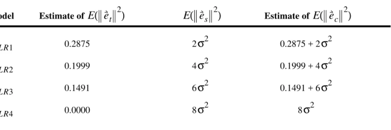
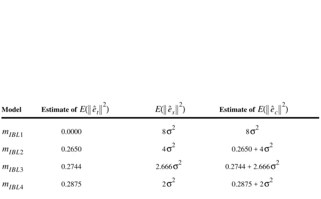
Kibler et al. (1989) report the results of an empirical comparison of linear regression and instance-based learning. The form of instance-based learning that they used was essentially what is called here . Let us consider their Experiment 1. In Experiment 1, , (Ein-Dor and Feldmesser, 1987), and (Kibler et al., 1989). Therefore . From Theorems 6 and 10, we see that linear regression will be more stable, for these values of n, r, and k, than instance-based learning. Kibler et al. (1989) did not use cross-validation testing, but they did report the error on the training set. They found that linear regression and instance-based learning had very similar training set error. We may take this to indicate that they would have very similar expected training set error. Although we do not know the level of noise , if there is a significant amount of noise, then Theorems 1, 6, and 10, taken together, suggest that linear regression will have lower cross-validation error than instance-based learning. This result must certainly depend on the data. For some data, linear regression will have a lower cross-validation error than instance-based learning. For other data, instance-based learning will have a

σ E e( _s ) X y, ₂ ( ) (X y, ₁) e_s (X y, ₂) X y, ₁ ( ) E e( _s ) e_s E e( _t ) E e( _s ) E e( _t )+E e( _s ) E e( _t )+E e( _s ) E e( _c ) m₂ n = 209 r = 4 k = 6 n k⁄ = 34.8 σ

lower cross-validation error than linear regression.

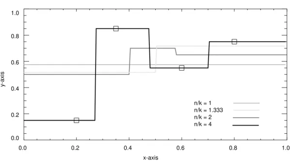
6 An Example

Let us consider a two-dimensional example. Suppose the training set consists of four points ( ) in :

(180)

Each point has the form . Our task is to form a model of this data.

Let us first apply linear regression. As discussed in Section 3, we are not limited to the given inputs . We may introduce an unlimited number of functions of . Let us consider here the natural number powers of :

(181)

Let us consider four different linear regression models, . These four different models are based on four different choices for the inputs:

(182) For example:

(183)

Our four models are:

n = 4 ℜ2 x x₁ x₂ x₃ x₄ 0.20 0.35 0.60 0.80 = = y y₁ y₂ y₃ y₄ 0.15 0.85 0.55 0.75 = = x_i,y_i ( ) x x x x_i x₁i−1 … x₄i−1 = i = 1, ,… 4 m_LR1,m_LR2,m_LR3,m_LR4 X_{i x} 1, ,… xi = i = 1, ,… 4 X₃ x₁, ,x₂ x₃ x₁0 x₁1 x₁2 … … … x₄0 x₄1 x₄2 1 x₁ x₁2 … … … 1 x₄ x₄2 = = =