A correlation equation to determine residential cooling energy consumption in Canada

Publisher’s version / Version de l'éditeur:

Vous avez des questions? Nous pouvons vous aider. Pour communiquer directement avec un auteur, consultez la première page de la revue dans laquelle son article a été publié afin de trouver ses coordonnées. Si vous n’arrivez pas à les repérer, communiquez avec nous à PublicationsArchive-ArchivesPublications@nrc-cnrc.gc.ca.

Questions? Contact the NRC Publications Archive team at

PublicationsArchive-ArchivesPublications@nrc-cnrc.gc.ca. If you wish to email the authors directly, please see the first page of the publication for their contact information.

https://publications-cnrc.canada.ca/fra/droits

L’accès à ce site Web et l’utilisation de son contenu sont assujettis aux conditions présentées dans le site LISEZ CES CONDITIONS ATTENTIVEMENT AVANT D’UTILISER CE SITE WEB.

Paper (National Research Council of Canada. Institute for Research in

Construction); no. IRC-P-3119, 1993-07

READ THESE TERMS AND CONDITIONS CAREFULLY BEFORE USING THIS WEBSITE. https://nrc-publications.canada.ca/eng/copyright

NRC Publications Archive Record / Notice des Archives des publications du CNRC : https://nrc-publications.canada.ca/eng/view/object/?id=50e630a5-161c-489d-970b-7d28ff81dcc1 https://publications-cnrc.canada.ca/fra/voir/objet/?id=50e630a5-161c-489d-970b-7d28ff81dcc1

NRC Publications Archive

Archives des publications du CNRC

For the publisher’s version, please access the DOI link below./ Pour consulter la version de l’éditeur, utilisez le lien DOI ci-dessous.

https://doi.org/10.4224/23000786

Access and use of this website and the material on it are subject to the Terms and Conditions set forth at

A correlation equation to determine residential cooling energy

consumption in Canada

A Correlation Equation to Determine Residential Cooling Energy

Consumption in Canada

Guy R. Newsham, Dan M. Sander, and Alain Moreau

ABSTRACT

We have developed a simple correlation equation for predicting residential cooling en- ergy consumption in Canada. Inputs

to

the equation are: interna! gains, envelope U-val- ues, glazing area, shading coefficient and cli- mate parame1:ers. Separate equations, of the same form, have been developed for both manu- ally vented and non-vented buildings. This pa- per describes the development of the seasonal cooling energy correlation equation, and com- pares its predictions with those of an hourly simulation model.

Guy R. Newsham is a Research Associate, lrnititute for &- search in Cornitruction, National Research Councü of Can-

ada, Ottawa, Ontario. Dan M. Sander ia a Senior Research O{ficer, Institute for Research in Construction, National Re-

search Councü of Canada, Ottawa, Ontario. Alain Moreau is a Research Engineer, LTEE, Hydra-Québec, Shawinisan,

Québec.

INTRODUCTION

The number of Canadian homes with air con- ditioners bas increased rapidly in recent years. For example, between 1988 and 1990 the num- ber of households in Ontario with central air conditioning rose from 6 percent

to

32 percent; 49 percent of homes built since 1988 incorpo- rated central air conditioners (Ontario Hydro 1990).

This increase in residential cooling is of par- ticular concem

to

those utilities seeking to re- duce network electricity use. Indeed, many utilities have initiated aggressive Demand Side Management (DSM) programs, with the aim of reducing residential electricity demand. These DSM programs often include cash rebates for the adoption of energy efficient appliances. However, the impact on residential energy con- sumption of replacing an existing appliance with a more energy efficient one is complex. For example, while a more efficient appliance

will consume less electrical energy, it will also

produce less heat. This reduction in internal heat gain will increase heating system loads in the heating season, and reduce cooling system loads in the cooling season. Depending on the building and the climate, the net saving in en- ergy consumption may be significantly differ- ent from the simple reduction in electrical energy consumption of the appliance. As part of a larger effort

to

address the impact of energy efficient appliances on network energy con- sumption, we were charged with developing a simplified method

to

predict residential cooling energy consumption in Canada. The calcula- tion of peak cooling loads were beyond the

40

The interactions between internal gains and building loads make it difficult for utilities to

predict future load growth and the impact of DSM programs. Hourly simulation models of building heat transfer can calculate the interac- tions well, but are typically difficult to use. For policy analysis applications, a better solution would be an appropriate simplified method for calculating building energy consumption. There would be some loss of accuracy at the level of an individual building. However, ifone is trying to predict the impact over tens of thou- sands of households, this loss of accuracy is off- set by the gain in simplicity. A simplified method could be easily incorporated into a spreadsheet, whereby a change in internai gain or other building parameters would produce a corresponding change in building energy con- sumption almost immediately.

A number of simplified methods have been developed that are capable of predicting build-

ing heating and/or cooling energy consumption

to within typically 15 percent of the value pre-

dicted by

an

hourly model. These methods fall

into two categories:degree-day and bin meth-

ods (Kusuda, Sud, and Alereza 1981, Gunter- mann 1981, Alereza 1985), and correlation equations (Peterson, Jones, and Hunn 1989, Sullivan et al. 1986, Sullivan et al. 1985, Parken and Kelly 1981, Barakat and Sander 1986).

Building Research Journal

Tb = Base temperature (in the simplest case equal to the design indoor temperature, Ti °C; and

Nd = Number of days incooling season.

Therefore, the basic degree-day method does not account for internai or solar gains, a seri- ous drawback. To include internai and solar gains, variable-base degree-day methods have

been developed in which the cooling degree

days are calculated

to

a base temperature de-

rived from the following equation (ASHRAE

1989):

(

2)

where

Qis = Mean sum of interna! and solar gains, W.

The bin method adds further sophistication. This method recognizes that using a single,

mean design outdoor temperature may be in-

adequate. A more accurate energy prediction is achieved by calculating cooling energy at sev- eral values of outdoor temperature. The sea-

sonal cooling requirernent for the building is then found from:

C

=

(Y Tl x nn + y ri x nri + y T.J x nT3 ... )

To calculate cooling coil energy, the degree- day method utilizes an equation of the follow-

ing form: where

(

3)

c

= HL X CDD X 24/1000 (1)

where

C = Seasonal cooling coil energy, kWh;

HL = Building heat loss coefficient in sumrner, Wt°C; and

CDD = Annual cooling degree days.

(la) where

T0 = Design surnmer outdoor temperature (T0 >Tb), °C;

"(I'j = Cooling coil load at outdoor temperature

Tj, kW;

nTi

=

Number of hours outdoor temperature is

at Tj; and

I.jnTj = Total number of hours in cooling season.

This method requires bin temperature data (giving n'IJ) for the location.

Correlation rnethods use statistical tech- niques

to

consistently relate building parame- ters (independent variables) to resultant energy consumption (dependent variable). For a particular location:

; Volume 2 Number 11993

Consistency can be achieved across geo- graphical locations only if the coefficients of the correlation can themselves be reliably corre- lated to climate parameters:

C

=

function (building parameters, climate)

(

5)

The main problem is the definition of suit- able building parameters as independent vari- ables.

At the onset of this project we were unde- cided as to which of the simplified methods to

pursue. Of the references listed, only Kusuda, Sud, and Alereza (1981), Sullivan et al. (1986), and Parken and Kelly (1981) dealt with residen- tial cooling. There was no method that was clearly superior when compared to an hourly model, and none of the methods had investi- gated parametric variations in internai gain to

the extent that we intended. In the end, we de- cided to pursue a correlation method, princi- pally due to our experience in developing these methods in the past (Barakat and Sander 1986). METHODS AND PROCEDURES

Hourly Simulation Runs

The EASI hourly simulation model was cho- sen to calculate the cooling energy consumption from which the correlation was derived. EASI employs the ASHRAE transfer function

method, and was originally developed by Public Works Canada. EASI was the model used by Barakat and Sander (1986) to develop a correla- tion method for predicting the utilization of in- ternai heat gains in off-setting heating load.

For this project, a modification to EASI was made which attempted to account for the win- dow opening behavior of occupants. In a resi- dence, the occupants may choose to open windows to cool the building through increased ventilation, before resorting to mechanical cool- ing. We modelled this response in the following way: ifthe cooling lond could be met by in- creased ventilation, then the ventilation rate was increased above the minimum infiltration rate to the ventilation rate that would satisfy the cooling set-point (up to a given maximum air flow rate); ifthe maximum ventilation rate did not meet the cooling load, then the ventila- tion rate remained at the minimum infiltration

41

rate (the windows were closed) and mechanical cooling took over. These assumptions are con- sistent with the ventilative cooling assump- tions made by ASHRAE (1989). They represent an occupant gaining the maximum possible benefit from increased ventilation by window opening and thus form a lower boundary to the cooling energy requirements.

The Modelled House

The bouse modelled in these studies was de- rived from the base case bouse used in the on- going development of the new Canadian Energy Code (Swinton and Sander 1992). The following parameters remained constant for all simulations:

• Floor Area,

Ar.

160 m2, square plan; • Wall Area, Aw: 184 m2_;

• Volume: 604 m3

• Thermal Mass: 60 kJl°Cm2 _floor area (interior);

• Thermostat: Heating, winter (Oct. - Apr. only) 22°C: Cooling, summer (May - Sep. only) 24°C;

• Max. ventilation: 0.2 m3_s·1_(win- dows open).

The following parameters were varied be- tween rune, over the given range of values, but remained constant for all hours of any particu- lar run:

• Internai Gains (incl. occupants), I: 0 - 12.5 W/m2_{, in 1.25 W/m}2 _incre- ments;

• Glazing (fraction of wall area glazed

x shading coefficient): 0 - 0.5, in steps of 0.1, glazing equal on all walls;

• HLF = mean U-value (incl. infiltra- tion) x

Aw

/ Ar.

0, 0.29, 0.58, 1.15, 1.73, 2.30, 2.89 Wl°Cm2•

The calculation of transmission losses and gains did not include the attic space above the ceiling.Although solar radiation falling on the roof does raise the temperature in the attic space, Canadian practice dictates that the attic

)

;

• 42

be well ventilated and the ceiling higbly insu- lated (U< 0.2 Wl'Cm2 . Therefore, heat gain through the ceiling was not considered a signifi.- cant component to the cooling load. Similarly, we did not consider solar gains through opaque wall elements, which have been shown, using DOE 2.lE, to be very small in Canadian cli- mates (Cornick 1993).

The range of parameters studied was far wider than that likely to be found in any sam- ple of Canadian homes. Therefore, any correla- tion which is accurate over this range of parameters is likely to be stable for any sample of residences to which it is applied.

Building Research Journal

To calculate infiltration in terme of a U- value:

where

(

6)

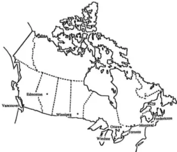
Figure 1. The eight Canadien cilles for which lhe correlation was derived.

would not be employed in residences during Oc- tober to April.

Uw

•

U-value due to infütration. W/°C;

Cp

=

Specific heat of air, J/lqfC;

p

=

Density of air, kg/m3 and F= Flow rate of infiltration air, m3s·1

Sensible cooling energy consumption was cal- culated for all combinations of internal gain, glazing area and U-value, giving a total of 462 runs for each geographical location. Runa were performed for the following locations: Frederic- ton, Montreal, Ottawa, Toronto, Windsor, Win- nipeg, Edmonton, and Vancouver (...Figure 1). This selection adequately covers the Canadian climatic range in the most populated areas. Two separate sets of runs were performed: first, assuming a bouse where the windows were not opened to exploit passive cooling (non- vented case); and second, for a house with the window opening behavior described above (vented case).

lt was assumed that the seasonal cooling en- ergy consumption could be reasonably calcu- lated from the sum of hourly cooling energy consumptions for the period May to September. For some combinations of parameters and cli- mate, the hourly model tnay yield a cooling load at other times of the year, it is reasonable to assume that, in Canada, mechanical cooling

RESULTS

The Cooling Correlation

The instantaneous (hourly) sensible heat bal- ance during the cooling season is given by:

8tot =g,+g,-l,

(

7)

where

Keot =-Total instantaneous heat gain, kWh/m2

Ki

=

Instantaneous internai gain, kWh/m2

g,

=

lnstantaneous solar gain, kWh/m2 l1

=

lnstantaneous transmission loss, kWh/m2

Ail gains are expressed in terme of floor area. If the room air temperature is below the

cool-ing set-point g101 wi11 result in a rise in room air temperaturc; ifthe room air temperature is above the cooling set-point then gto1 becomes

the instantaneous cooling load.

Therefore, over the whole of the cooling sea- son:

Volume 2 Number 11993

where

Cr= Seasonal sensible cooling energy consump- tion, kWh/m2;

Gi

=

Seasonal total of intemal gains, kWh/m2;

G.

=

Seasonal total of solar gains, kWh/m2; and

L1 = Seasonal transmission losses, kWh/m2

(seasonal transmission gains for Canadian climates are insignificant, less than 100 kWh in most cases; see also Jones and Howell (1986)).

Note that Cr is the cooling coil energy con- sumption. To obtain the system (or billing) en- ergy consumption, one should use the following equation:

_ .2!_

Cay.- COP

(9)

where

Cay, = System (or billing) energy consumption, kWh/m2; and

COP •Coefficient of performance of system.

Gt

depends on the occupancy schedule and

the internal gains and is described in the fol- lowing equation:

(10)

where

He

=

oocùpied hours in 5 cooling months; in this case, all hours May - Sept.

=

3672.

a.a

nd Ltare climate dependent parameters.

G,is described by the following equation:

43

W₁

=

Fraction of wall area glazed.

Lt

is described by the following equation:

L,= kt x HLF (12)

kt is a climate-dependent heat loss parame- ter, normalized to tloor area. It is the value that the term

CC.CU, G.,

Gt> -

Ci( 0,

G.,

Gt>

I HLF] tends to, calculated by the hourly model, as G.and

Gt

tend to their upper limits. This is illustrated in Figure 2 for Toronto. After trying

many parameter combinations, k 1was found to be accurately correlated to climatic parameters in the following way:

k1

=

a0 + a1·HDD2 + ·VS + as ·VSS

+ a4 • CDD1+ a5 • CDD2 +a6 ·DRNG

(13) where

HDD2 ..Annual heating degree days (base 18.3 oc);

VSS ..Mean daily solar radiation on south vertical, MJ/m2;

CDDI

=

Annual cooling degree days (base 10°0);

CDD2 ..Annual cooling degree days (base 18.3 oc)

DRNG •Mean daily temperature range for July (oC);

VS •VSS + VSN + VSW;

VSN •Mean daily solar radiation on north verti- cal, MJ/m2;

VSW

=

Mean daily solar radiation on west verti- cal, MJ/m2; arid a0 ==-65.8451, a1

=

0.007881, a2

=

15.4141, G,

= (

SllC X SC X Wg ) Ar where (11) a3 = -25.8951, a4 = 0.02770, a5 = -0.1427, ae = 0.3416.

Figure 3 compares

kt

derived from the hourly

model and kt derived from the climate correla- tion of Equation 13, for all eight locations.

Suc= Total solar gain on all vertical surfaces dur-ing the cooldur-ing season (May - Sept.), kWh; SC = Shading coefficient; and

We reasoned first tbat the ratio of mechani- cal cooling to total gain, CIGtot (Gt.ot =

Gt

+ GJ, would be a good dependent parameter, since it

Gtot 1 1 G G

L,-J]

4 (-

[.;-44

would always lie between 0 and 1for both the vented and non-vented cases, and that baving such simple limits for both cases would facili-tate finding a correlation appropriate to both.

Building Research Journal

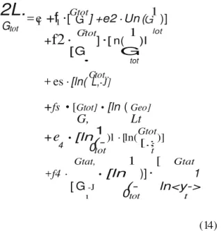
2L.

_{= e}

_+f

_·[Gtot

] +e2 · Un ( 1 )]

8 lot

+

f2 ·

Gtot] ·[ n( 1 )l

[ G G

After trying many independent parameter com- binations, guided by those parameters used by Barakat and Sander (1986), we found that

Ctr'Gtot was a function of the inverse of the total gain (llGtot), the gain-to-loss ratio (GtoJLt), and the ratio of total gains to solar gains (Gtot/G.).

Linear regression on combinations of these three parameters to C/Gtot yields an equation of the following form:

• tot + es ·[ln( Gtot..

+

fs • [Gtot] • [ln ( Geo] G, Lt +

e

• [ln 1 )l · [ln(Gtot)] 0tot t Gtat, 1 [ Gtat +f4 · • [ln )] · 1 [ G -J (- ln<y-> 1 0tot t (14) -10 i§ -15 "O

Toronto - no vent

WgxSC where

and

fi

are climate-dependent coefficients.

Once the coefficients 0ï and

fi

had been gener- ated for all eight locations we found that Equa- tion 14 could be simplified since: e2, e3,and e4

were linearly related to e1; f2 was linearly re-

lated to f1; and f4 was linearly related to f3:

S. 7 10.00

Internai Gains, W/m2

Figure 2. Derlvation of the heot loss parameter kt, curves for a single value of HLF (1.15), are shown.

35

5

O'-l"- -.- ,s ro .---.,.- 4,0

Kt (hourty modal)

Figure 3. kt derived from dimate correlation vs. kt derived from hourly modal,for all eight locations.

Non-vented: e2

=

-0.1655 + 0.1719 ·e1 (15a) e3

=

0.2347 - 0.4522 · e1 (15b)

e

4

=

0.03783- 0.08003 ·e1 (15c)

f2

=

0.03170

+

0.2259 .

f1

(15d)

f

4

=

-0.01594 + 0.2249

·fa

(15e) Vented: (16a)

e

3

=

0.2286- 0.7045 ·

e

1 (16b) e4

=

0.03045-0.1191 ·e1 (16c) f2

=

0.02954 + 0.2061 .

f1

(16d)

Volume 2 Number 11993

f,

=

0.000278 + 0.2072 .

fa

(16e)

These relationships are illustrated in F"igures

4 (a) ·(•) . Therefore, for consistency across geo-

graphical locations, climate dependence for

only 3 coefficients (ei. fi. and f3) need be

de-rived. Mer trying many parameter combina-tions, we found that ei. f1, and f3 were

correlated to climate parameters by the follow-

ing set of equations: Non-vented:

e1 =ao+a1 · VS + a2 • VSS + a3 • CDDl

+ a4 • CDD2 + a5 • CDHl + as· DRNG

(17)

where

CDHl = Annual Cooling Degree Hours (base

26.7 °C); and ao =26.0884, a1 = -0.9139, a2 = 0.7031, aa =-0.01372, a4 = 0.02067, a6 = 0.006446, aa = -0.6308. f1

=

ao + ai ·VS + a2 ·VSS + a3 ·CDDl + a4 • CDD2 + a6 • CDHl + as ·DRNG (18) Vented: e1= a0 + ai ·VS+a2 · VSS +aa · CDDl + a4 • CDD2 + a6 • CDHl + as· DRNG (20) where o0 =23.0141, o1= -0.8474, a2 = 0.6758, a3 =-0.01187, 04 = 0.01825, a5 = 0.005293, aa = -0.5414. f1 = ao + ai ·VS+a2 ·VSS + aa ·CDDl + a4 • CDD2 + a6 • CDHl + as· DRNG (21) where ao =-0.5568, a₁= 0.04818, a2 = -0.05074, a3 =-0.0003145, a4 = 0.001088, a5 = -0.0001684, a6 = 0.03147. fa = a0 + ai · VS +

a

2 • VSS + aa ·CDDl + a4 ·CDD2 + a6 • CDHl +as · DRNG (22) where where a0 =5.07264, o1= -0.2343, o2= 0.2090, ao =-6.06729, a1= 0.2349, a2 = -0.1976, o3 = 0.002864, o4 = -0.004017, 06 = -0.001767, oa = 0.1767.

fa

= ao + ai ·VS+a2 • VSS + aa ·CDDl + a4 ·CDD2 + a6 • CDHl + aa ·DRNG (19) where oo =-0.6555, o₁= 0.02538, o₂ = -0.01831, oa = 0.0006844, o4 = -0.001820, a5 = 0.0001315, a6 = -0.001379. aa =-0.002028, a4 = 0.002298, a5 = 0.001342, ae = -0.1264.

The climate parameters VS, VSS, HDD2, CDDl, CDD2, CDHl and DRNG can be found in data-sets published by ASlffiAE/IES

(ASHRAFJIES 1989) and Environment Canada

(Tsi-Cbih 1991). Table 1 liste these climate pa-

rameters for the eight Canadian locations spe-

cifically addressed in this paper. Figures 5 (a) •

(c) illustrate the relationship between elt flt fa derived from the individual regressions for each location, and the elt f11 fa derived from the

e4•0.0J045·0.1191

0

el 1

l

1 ;

46 Building Research Journal

l

0.1.--- 0.1-.---,,--- -.., 0.0 ·-···-..-...-- ·--···-..·-··-··--..·-··-·--·--···t-·-···..·-· -0.1 -0. .o -0.8 0.7

(a)

o.o ----·-·-...---·-·-··....

---r

-

--j 'ijl -0.1 -02 -0. .o 0.7 0.5 0.4 ';! 0.3 0.6

(b)

o.s 0.4 c

"'

0.3 c 0.2 0.1 1 02 1 0.1 e3 • O 2266 • 0,7045 e1 1 0.0 ·-·-·-· · · · ---...-· ···-··-····-··--···--·

---·---!

o.o ...-...---....

·--·

·

i--··---

i

·

..

--0.!1+.o=--.---0".'s:---.----,0,.,-e=---.--,-.4,--.---0:".2',--.---0:+.-o:=--.---:o<.2

e1 -0.8 -0.6 el -0.2 -0.0 0.11 0.07 1i 0.05 0-11 0.09 0 OJ)7 0

(c)

_{1li 0.05} 0.03 1 •••••••••01 ,.•••,.•• •••· 1.-·- - •- ---·•••••• ••n••·--i · ••-0.03

..

... .

...

.

...

..

.

...

-

...

,.

...

-

..

-+...

...

..

0.01 1 0.01 -0.8 -0,6 -0,4 -0.2 [ -0.0 0.2 "°-0 :1.<.-o --.---0"e.'=--.----,0".':---.--,-_4,--.---_-0:.-.-2::-.---0:"."o=-.--:01.2 e1 0_15,.. ---.- ---. 0.13 el 0.1 0.13 0.1 1 0.09 0.07 o.os o. ...

(d)

0.11 0:09 0.07 0.05 0.03 0.01

-

..

--··-· ·· .1 -0.0 0.1 02 0.4 0.5 11 -0.0"1_2 _{-0.0 0.1 0.2 o.:i} 11 OA 0.5 0.02.---!--- o. o.oo -001 :!: -0.02 -0.03

!

0 0 1 · -·-···-..···..---·-·· -·-·· 1 001594 • CL.n.4.t" O.Q1 O.ClO -0.01 :!: -Q,02

(e)

_-0.03 -0.04 13

Non·ventecl

Figure 4 . The linear relallonshlps be-

lween correlallon coefficients for bolh lhe non.Yented and vented cases.

13

Vented

0 ···_· ··-..:.·

!

.··-··- _····_····-···-...--··

----

..-...

..----

-*"··· _··· ·-·-·--0.1 --·----· M ••

o.

i

1

Volume 2 Number 11993 0.25,...---- ---.-- -47 0.25--- 0 -·-·-··..·-·--···..·-···· ··... ··-· -···

'*

-0.25 Cl

(a)

0 ---·..·---..···---·""""'""'''"'"'"-·-··"'"'''''"''""''''"'' ... -0.25 8 Cl -0.5 'ài -0.75 -1.,'--- - - -- - - - --i---,---O. 5 -0.5 -0.25 5 e1 (individual) 0.75.-- ---.,.--- --- -0.5 '2

li

Gl ·- -0.5 :8.. 'ài -0.75 -1_ --.- -0.-5 ...----0.5 -.---0.25 -.---t- ..--o-1. e1 (individual) 0.75--- --0.5 .!!! 0 u _0.25 Cl E ;:::::

(b)

C1l 0.25 n;

!

-0 ... ...,.._,_,...-...

-

_{0 -·--··--·-·-··} ·0·2.n.25 o. 5 11 (individual) 0.5 o. 5 O. 5 11 (individual) 05. o. 5 025.---, ---l 0.25 ..--- ---...,,, 0 ...

!.

.

....

.

....

...

-

....

...

i

.!

1

(c)

.!!! ê 8

.!

0 ..._ ... ... i -0.25 ' i -0.25

!

-0..5 -0.25 1 f3 (individual) o. 5 -0. .5 -0.25 f3 (indMdual)

o

.

5

Non-vented

Vented

Figura 5. Correlation ccefficlenls darivad Fran the dimala correlation vs. oorralation coefficients of the Individuel regressions, b- all eight loc:ations.

48 Building Research Journal

DISCUSSION Accuracy of fit

F"igures 6 (a) • (c) show the annual cooling en-

ergy consumption calculated using the correla- tion vs. EASI annual cooling energy

consumption, for the base case house under both vented and non-vented conditions for Toronto, Winnipeg and Vancouver; results for all combinations of internai gain, U-value and glazing are shown. In the vast majority of cases, the differences are less than 10 percent. The absolute differences are, again in the vast majority of cases, less than 1000 kWh/year; with a COP of 3 and an electricity rate of 7.5

/kWh, this amounts to an error of $25/year.

Tables 2 and 3 show the mean absolute and

percentage di:fferences for all eight cities for both the vented and non-vented cases. The mean percentage di:fferences are less than 7 percent in all cases, and in most cases less than 5 percent. Mean absolute di:fferences are less than 1000 kWh in all cases. Although, as might be expected, cooling energy consumption for the vented cases is lower than for corre- sponding non-vented cases, the mean :iercent- age di:fferences in the vented cases are

generally higher. This is due to the extra de- gree of freedom introduced by the window open- ing option.

Limitations

The correlations have been derived for a bouse of a single form and thermal mass. Therefore, although the correlation can be ap- plied to any size bouse, it should only strictly be applied to bouses with equal glazing on all facades, and to bouses of thermal mass 60 kJt'Cm2• However, a large fraction of Canadian wood-frame bouses do fit into this mass cate- gory. Another limitation is that many of the as- sumptions made for the base case house, particularly those referring to the heat transfer at opaque surfaces, are specific to Canadian construction and climate.

The correlations are very sensitive to the in- put climate data. For reliable results, it is ex- tremely important to use only the input climate data supplied in this paper (the data used to de- rive the correlations are ten year averages), the data from which the correlations were derived. While this limits the applicability of the correla-

tions to those cities specifically listed in the re- port, these cities are representative of the most populated areas of Canada. The same limita- tion exists for the correlations of the

ASHRAFJIES 90.1envelope compliance proce- dure (ASHRAE/IES 1989).

Internai Gain Schedule

The correlation was developed for a con- stant, 24 hour internai gain schedule. However, runs for a subset of climates using a more typi- cal residential internai gain schedule (Barakat and Sander 1986) (Figure 7), with the same total

internai gain as the constant schedule, showed that the correlation did not change signi:fi- cantly.

Human Behavior with Respect to Air Conditioner Use

Recent studies (Kempton, Feuermann, and McGarity 1992, Lutzenhiser 1992) indicate that the interaction between residential occu- pants and their air conditioning systems is far more complicated than that modeled here. Here we model a "thermostatic" control strat- egy, in which the system cycles on and off auto- matically to attain a pre-set room temperature; in the vented case, the initiation of this thermo- static control is delayed by opening windows. While "thermostatic" control may be the control strategy anticipated by manufacturers, the above studies found that, in the case of room air conditioners, a majority of users adopted a "manual" control strategy. The "manual" con- trol strategy involved the user cycling the ma- chine on and off as desired; when on, the thermostat was usually set to provide continu- ous operation. In most cases, the "manual" strategy resulted in a lower energy consump- tion than the "thermostatic" strategy. However, the parameters which stimulate users to adopt the "manual" strategy, and to decide when to cycle the air conditioner, have yet to be deter- mined. Therefore, at present it would be impos- sible to model this kind of control in a study of this kind.

Latent Cooling

The above correlation predicts only sensible cooling energy consumption. We also investi- gated methods of calculating latent cooling en- ergy consumption, for example CHBA (1991). However, the extra complication incurred in generating an accurate latent cooling energy

Volume 2 Number 11993 49

Toronto - no vent

40,--,....-,....-,....- ,....- --.:.:.;:...::....--... ...•-'

...

36 / ,W %

I

:

:

_:

:

:

:

::

-/-/

ll

_g 8 E 16 12 8 4 40 36 32 28 en 24

(a)

_{'""- Eil! 20} 8 16 12 8 4

Toronto - vent

10% Q-!"----.r----.- , 1r 16 2.0. -- 4 -EASl,kWh {Thousands) 2 r 832 --3..6.----4t0 0 _{12 16 20 4 28 32 36 40} EASl,kWh {Thousands)

Winnipeg

-

no vent

40,--,....- , 10_%-=

..

.

/

.

.

/ 36 / ..._....10%

Winnipeg - vent

40 36 10% 32. ...,.. ...

;I

/

/ /:::

/ /

/

12 8 4 32 28

(b)

₃

₂₄

il:

12 8 4 0· :..-,..----.- 12 -16 20 -.4 -EASI, kWh (Tuousands) 8 -32 36 --440 0 _{12 16 20 4 28 32 36 40} EASl,kWh {Thousands)

Vancouver - no vent

40..-- -..,,-'-'----.,. ,

.

.

····"'

w

.

.

/ /

/ /

..

,.

i

20

8

Ë

16 12 8 4 40 36 32

(c)

28 24

=

ê

-

0 20 8 Ë. 16 12 8 4

Vancouver - vent

10% . O.f'IZ.--.,....---.- 12 -16 2r0---r4 2r8 32 3r6 ----4-!Q EASl, kWh {Thousands) 0 _{12 16} 20 4 8 32 36 40 EASl,kWh {Thousands)

f igure 6. Coollng energy consumption oolculated using the correlation vs. EASI coollng energy con-

sumpllon, for ail build ing parameter variations, for both the vented and non-vented ooses, in Toronto, Winnipeg, and Vancouver. 10 % differenœ levais are indiooted.

50 Building Research Journal

Table 1. dimate parameters for 8 Canadlan clties.

City HDD2

vs

vss

CDDl CDD2

cnm

DRNG Fredericton 4840 _{18.21 9.20 928 124 319 12.7} Montreal _{4615 17.65} 8.67 1201 226 315 10.6 Ottawa 4758 18.27 9.13 1164 212 407 11.4 Toronto _{4218 17.37 8.34 1201 224 510 12.5} Windsor 3687 18.82 8.86 1535 371 781 10.9 Winnipeg _{5965 21.11 10.99 1000 169 479 12.5} Edmonton 5938 21.06 10.97 592 27 88 18.1 Vancouver _{3112 17.12 8.25 859 80 8 9.1}

Table 2. Mean perœntage and absolute differenœs between Table 3. Mean perœntage and absolute differenœs between lhe annual coollng energrc consumptlon oolculated by an lhe annuel coollng ene:r; cansumptlon oolculated by an hourly modal and lhol co culated uslng the correlotlon, for oil hourly model and that ca culated uslng lhe cOl'relatlon, for ail building porometer variations for o non-venled house. building porometer variations, for a vented house.

City

%

Mean Differences

absolute1 kWh/l'.ear

City

%Mean Differences_{absolute1 kWh/l'.ear}

Fredericton _{2.7 325} Fredericton 2.9 344 Montreal _3.0 474 Montreal _{3.7 522} Ottawa 3.2 393 Ottawa 4.3 490 Toronto _{2.8 391} Toronto 4.0 506 Windsor _{3.3 569} Windsor 6.8 971 Winnipeg _{3.4 521} Winnipeg 3.4 480 Edmonton _{4.7 728} Edmonton 6.9 897 Vancouver 5.7 781 Vancouver 6.5 641 llmeof day

Figure 7. Typiool residential internai gain schedule.

2 l.t' .-

- 1.e-u .-

-

.-

-

1.2-,.

0.lt' Oh -.-

---

-OA" o.2' 1 2 3 4 5 8 7 • 1 10 11 12 13 14 15 1• 17 11 11 211 21 22 23 24