A New Specification-based Qualitative Metric for Simulation Model Validity D. Foures, V. Albert, A. Nketsa
CNRS; LAAS; 7 avenue du colonel Roche, F-31077 Toulouse, France Université de Toulouse; UPS, INSA, INP, ISAE; LAAS; F-31077 Toulouse, France
dfoures@laas.fr, valbert@laas.fr, alex@laas.fr
Abstract
Informal validation techniques such as simulation are extensively used in the development of embedded systems. Formal approaches such as model-checking and testing are important means to carry out Verification and Validation (V&V) activities. Model-checking consists in exploring all possible behaviours of a model in order to perform a qualitative and quantitative analysis. However, this method remains of limited use as it runs into the problem of combinatorial explosion. Testing and model-checking do not take into account the context of use objectives of the model. Simulation overcomes these problems but it is not exhaustive. Submitted to simulation scenarios which are an operational formulation of the V&V activity considered, simulation consists in exploring a subset of the state space of the model. This paper proposes a formal approach to assess simulation scenarios. The formal specification of a model and the simulation scenarios applied to that model serve to compute the effective evolutions taken by the simulation. It is then possible to check whether a simulation fulfils its intended purpose. To illustrate this approach, the application study of an intelligent cruise controller is presented. The main contribution of this paper is that combining simulation objectives and formal methods leads to define a qualitative metric for a simulation evaluation without running a simulation. Keywords: Experimental Frame, Abstraction, Input/Output Automata, Compatibility
1. Introduction 1.1. Context
In [1] it is stated that a model abstraction is valid if it maintains the validity of the simulation results with respect to the questions the simulation is supposed to address. Hence, the validity of a model should never be assessed in isolation but should always be envisaged in relation to the context in which the model is experimented, i.e. the purpose of the simulation. Traditional Modeling and Simulation (M&S) practices describe abstraction choices when building up a model to provide documentation of its "domain of use" as suggested in [2, 1, 3]. These practices do not follow the same process for the intended purpose of the simulation. However, simultaneously conducting the same process for the model and its context would make it possible to define a priori the sufficient and necessary model required to reach an intended purpose and to check a posteriori whether a model can be used in various contexts. Thus, challenging issues in M&S are mostly related to their specification/documentation, the capabilities of the model and the properties expected from this model to achieve the simulation purpose.
1.2. Framework
We retained the Theory of Modeling and Simulation (TMS) developed in [4]. Zeigler established a framework which provides a precise definition of the entities involved in the process of modeling and simulation. We consider this framework as an excellent base for structuring modeling and simulation applications. It highlights relationships between the intended purpose of the simulation, the system which is represented and the simulations themselves. TMS is not the only existing framework available to describe dynamic system modeling. It can be compared with other work which has been published concerning the community of Verification, Validation and Accreditation (VV&A) of simulations as in [5, 6]. The experimental frame is one of the entities that have been introduced in the TMS to make a distinction between the model and the experiment. The experimental frame can be viewed as a system which interacts with the model in order to answer the questions raised by the simulation purpose. Then it consists in stimuli injected into the model inputs, observation of the model outputs and constraints to determine whether the model outputs "fit" some acceptance conditions. The experimental frame concept has been used for the simulation of embedded systems engineering in [7], for ecology systems in [8, 9] and for environmental processes in [10]. In [8], Traoré and Muzy pioneered a formal definition of the experimental frame. Our approach relies on this definition. However, this definition does not allow formal verification of the behavioural compatibility analysis between an experimental frame and a model. Such an issue is of paramount importance in order to know whether a model within an experimental frame can address the questions raised by the simulation purpose. Our approach is model-based. Therefore the experimental frame and the studied system are represented by their models. In this paper to avoid repeating the model word for both the system and the experimental frame, we are going to use a model for the system under test and experimental frame for its model.
1.3. Novel concept and its benefits
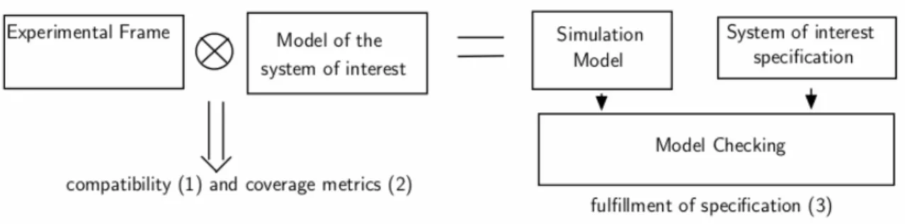
The novel concept relies on building a simulation model which specifies the model behaviour under the conditions of the experiment. This model is obtained by composition of the system model of interest and the model of the context within which that system is studied, i.e. its experimental frame. In a simulation-based development methodology, the intended purpose of the simulation would usually be to check that some requirements on the real system are met. The simulation model and the simulation intended purpose can then be input into a model checker for quantitative analysis. This idea is illustrated in Figure 1.
Figure 1. Novelty of the concept
A simulation scenario consists of a trajectory injected into the model inputs and a path of interest observed on the model outputs. Typically a simulation is not comprehensive in the sense that it does not explore all possible trajectories of the model. A simulation scenario restricts the model to a subset of evolutions the model may produce. Then the simulation requires metrics which capture (1) the applicability of a scenario to a model, i.e. a set of stimuli can be accepted by the model and the model produces expected outputs, (2) the reliability of the simulation results, i.e. to what extent the state space of the model has been explored by the simulation, and (3) whether certain requirements of the real system are met by the simulation model.
Metrics (1) and (2) can be measured by composition of the system model of interest and the model of the experimental frame, and metric (3) can be measured by checking the simulation model against the specification of the system of interest.
1.4. Formal specification languages
TMS also offers a specification language for models called Discrete Event System Specification (DEVS) using precise operational semantics thanks to an abstract simulator which establishes formal rules for executing a DEVS model. It is important to highlight that TMS is based on a general system theory. In this way, many types of systems can be modeled within TMS. TMS has given rise to many subclasses such as Cell-DEVS for cellular automata, DTSS for discrete-time systems and DESS for differential equation systems. However, DEVS is not used here as it does not support model checking because the state space of a DEVS model is infinite. State space exploration techniques and qualitative properties analysis can be supported by Finite and Deterministic DEVS (FD-DEVS). However as far as we know, there are no tools supporting FD-DEVS models and temporal logic.
Automata are a subset of DEVS. Automata theory is suitable for state space exploration and quantitative properties analysis with temporal logic and it supports well the composition of automata. With Input/Output Automata (IOA) we capture the temporal I/O behaviour of the model and the experimental frame. By composition we check whether the automaton which describes the trajectory injected into the model inputs can be accepted by the automaton describing the model of the system of interest and whether this set provides a path of interest observed on the model outputs. In [11], the authors use synchronous products of automata for composition. Behavioural incompatibility is detected if the product is zero. However this approach does not allow the cause of that incompatibility to be detected. Our synchronous product is based on the work of [12] which relies on an "optimistic" view of composition and offers the possibility to detect illegal states leading to possible incompatibility. Our composition adds another dimension, i.e. while two components can be synchronized and therefore compatible, we can highlight which part of the model is overlooked thanks to the synchonous product. Composition results in a new automaton which describes the behaviour of the simulation model which is checked against the requirements that the system under study must fulfil. The latter are described with Linear Temporal Logic (LTL) [13] properties. An LTL formula is interpreted on infinite words which do not include time as a first-class variable. State space exploration with linear temporal logic based on automata theory can be solved using UPPAAL [16]. Moreover, UPPAAL supports timed automata and event-clock automata specifications.
This paper is organized as follows. Section 2 gives an overview of related work. Section 3 includes a description of the M&S framework, experimental frame and IOA. Section 4 states the main contribution, defining a trace inclusion property with Input/Output automata. Section 5 describes steps
and an algorithm to conduct compatibility checks. Section 6 introduces an example of use of this approach. Section 7 gives a conclusion and anticipates future work.
2. Related work
Combining simulation with formal methods has been extensively investigated. We present our contribution in this context.
In [17], a model checker is used to automatically drive the SIMSAT simulator to check operational plans. In contrast to the verification of operational plans, our proposed approach has a general scope, being applicable to simulation models of any system and a set of requirements to be verified.
In [25] the authors use a model checker to generate all possible simulation scenarios and then optimise the simulation of such scenarios by exploiting the ability of simulators to save and restore visited states. Our approach is quite different because we have defined some metrics for evaluating simulation without running it.
In [18], the authors make the following observations: functional errors are not eliminated by synthesis and not detected by a formal verification based on test equivalence. These errors result from incorrect specifications, a misinterpretation of specifications, etc. They highlight the limits of formal verification (equivalence checking, model checking, theorem proving) in the context of validation. They use a semi-formal approach, initially proposed by [19], based on the notion of metric coverage coupled with simulation. The objective is to achieve understandable validation without duplication of effort. The approach combines symbolic simulation, model-checking and the generation of test vectors based on coverage analysis to minimize unwanted portions of the system. The authors advocate the definition of metrics at different levels of abstraction: on the code, the system structure, its state space, functionality and specifications.
In [20], the authors propose model checking to guide the simulation process and improve coverage. Coverage metrics are measured during the validation session and model checking is invoked when coverage is insufficient to reach uncovered parts of the state space more quickly. Invoking model checking is dynamically controlled during run-time.
We positioned ourselves relative to these works by considering two key differences:
• In current practice simulation, runs are actually performed: in contrast, our approach aims to verify before simulation whether a simulation behaviour (i.e. model + experimental frame) can be used for the intended purpose of the simulation which is derived from requirements on the real system.
• Using formal methods, all possible simulation scenarios are exhaustively explored: our approach makes use of the intended purpose of the simulation to investigate only that part of the behaviour of the simulation (that portion of the state space) which is of interest for the intended purpose.
3. Framework for the preparation of models and simulations 3.1. TMS
In [4], a new way of providing a model description is proposed and the question of knowing whether this model is a true representation of the dynamic behaviour of the system from a given perspective is asked. The basic principle of the M&S process described by Zeigler involves the separation of the model and the simulator. The basic entities of the M&S process are the system, the model and the simulator (Figure 2).
The system is the real or virtual element used as a source of observable data and subject to modeling. The model, also called system substitute, is a representation of the system. It usually consists of a set of instructions, controls, equations or constraints designed to generate its behaviour. The simulator is a computer system executing the model and generating its behaviour based on model instructions and injected inputs. This set is reorganised to integrate the experimental frame (EF). The
latter is a specification of the conditions under which a system can be observed or experimented. It is an operational formulation of the objectives which the development of the M&S application supports. There may be several experimental frames for the same system and the same experimental frame may be applied to several systems.
Figure 2. M&S process and its entities
It should be pointed out that the experimental frame transforms the objectives used to focus model development on a particular point of view, into specific experimental conditions. A model must be valid for a system in such an experimental frame. An operational formulation of the objectives is produced by matching the output variables with measurements of the system’s effectiveness in accomplishing its function. These measurements are called outcome measures.
Modeling is the relationship between a model, a system and an experimental frame. The validity of a model is the basic concept of the modeling relationship. Validity refers to the degree to which a model faithfully represents a system in an experimental frame of interest. The relation between a model and a simulator is simulation. The correctness of the simulator is the basic concept of this relation. A simulator correctly simulates a model if it guarantees a faithful generation of model output values given the model state and the input values. This relation refers to the principle of separating concerns about model design and its implementation.
3.2. Experimental frame
An experimental frame features three components as shown in Fig. 3: a generator, which generates a set of input segments for the system; an acceptor, which selects the data of interest to the system while monitoring whether the desired experimental conditions are complied with, and a
transducer, which observes and analyses the output of the system. Mapping between output variables
and outcome measures is carried out by the transducer.
An experimental frame is given in [8] as a structure where: EF = 〈T, IM, IE, OM, OE, ΩM, ΩE, ΩC, SU〉
• T is a time base,
• IM is the set of Frame-to-Model input variables, the set of model stimulation ports,
• IE is the set of Frame input variables, the control input set,
• OM is the set of Model-to-Frame output variables, the set of model observation ports,
•ΩM ⊆ (IM, T) is the set of segments injected into the model inputs,
• ΩE ⊆ (IE, T) is the set of admissible input segments for the experiment,
• ΩC ⊆ (OM, T) the set of segments observed on the model outputs,
• SU is a set of conditions, also referred to as summary mappings, which establishes relationships between inputs and outputs within the frame.
Figure 3. The experimental frame and its components
Typical experimental frame components can be found in [4] in chapter 14. For example, typical generator functions are sine wave, square wave, step ramp, periodic arrivals.Typical acceptor functions are steady state, transient. Typical transducer functions are throughput, turnaround times, elapsed times, rates, averages.
It has been seen that the experimental frame features data gathering (statistics, performance measurements, etc.) and behavioural control (initialization, termination, transient state removal etc.). Again, an experimental frame can be seen as a system that interacts with the system or the model to obtain data of interest under certain conditions. Hence, defining boundaries between the experimental frame and the model is essential to clearly distinguish between what drives the model, what can be observed as output, and the model itself. This has been illustrated in [3].
3.3. Input/Output Automata
We use input/output automata (IOA) [21] to describe the dynamics of models at a quite abstract level that is independent from an encoding language.
Definition 1 (IOA). It consists of the following structure:
A = 〈D, X, Y, dom, S, σ, Σ, δ, s0〉 where • D is a set of data types (integer, real, string, etc.),
• X is a finite set of names representing the set of input variables, • Y is a finite set of names representing the set of output variables,
• dom : X ∪ Y → D is the typing function which allocates a type of data to each variable, • S is the set of states,
•σ : S → ((X ∪ Y) → dom(X ∪ Y)) is the configuration function, i.e. mapping of values with the typed input/output variables for each state.
• Σ is the set of event names. These names are the state transition labels. e is the set of non-observable events.
•δ⊆ S ×Σ× S is the transition relation, a transition identifies a change to the inputs, the outputs or the states.
•s0 ⊆ S is the set of possible initial states, the states in which the automaton can be if no inputs have yet been transformed.
X ∪Y ∪ Σ is the vocabulary used to define the automaton. For the sake of simplicity, we will assume that the names used in the vocabulary are unique.
Example. Let us consider a communication system with a shared memory which implements a FIFO
(First In First Out) scheme, the behaviour of which is described by the reachability graph in Figure 4. In this example, a variable queue is defined to describe a sequence of messages. This variable is declared as a table of length 2. Each place of the buffer is set to 1 if there is a message, or 0 if not. This automaton has an initial state s0, where the sequence is empty (e.g. σ (s0) = (0, 0)). The set of state S is
{(0,0), (0,1), (1,0), (1,1) }. These states are connected by transition relations. These transitions are labeled by the events recv and send which respectively add a message to the head of the sequence and remove a message from the sequence.
Figure 4. Reachability graph of a shared memory communication system
Definition 2 (Run (or trace)). An IOA run is a sequence (finite or not) σ (s0) →l0 … σ (si) →li … where siis a state (s0is an initial state) and liis an event name such that any (si →li si+1) of a run is a transition of the automaton. A run can also be defined by a path taken from the computation tree of an automaton. "Run" can also be called "trace".
4. Our contribution on verifying trace inclusion
4.1. Objective of trace inclusion
ΩIEF are the simulation results that the experimenter wishes to observe, whereas ΩOEF are the stimuli injected into the simulation. Similarly, ΩIM are allowable inputs of the model and ΩOM are the possible simulation results.
Definition 3 (EF-Model behavioural compatibility). We state that an experimental frame can be
applicable to a model if their behaviours are compatible, i.e.: ΩOEF ⊆ ΩIM
ΩOM ⊆ΩIEF
The next section introduces a formal way for using IOA in order to check EF-Model behavioural compatibility.
4.2. Behavioural compatibility
A Temporal Interfacing Constraint (TIC) is an execution property defined with respect to a given vocabulary (names of events and input/output variables).
The properties of invariants are constraints on the configuration function. For example, let us consider altitude as an input variable of the automaton’s vocabulary. The constraint "variable altitude is positive or zero" is an example of an invariant. The automaton that satisfies this invariant includes an integer input variable called altitude and a configuration function σ such that, for any state s, σ(s)(altitude) ≤ 0.
The temporal properties are constraints which link the configuration and the transitions. There are two separate types of time-dependent properties:
• linear versus computation tree: refers to the constraints on all executions of the automaton versus those on the computation tree taken from the automaton,
• past versus future.
For example, consider the Boolean output variable alarm in the vocabulary of an automaton: "If the value of alarm is true in one state of the execution, then there is a previous state in the execution where altitude ≤ 10" is a linear time and past property.
"If altitude ≤ 10 in one node of the computation tree of an automaton, then we should be able to find a path and a subsequent node in the path which satisfies alarm = true" is an example of a computation tree and future property.
Definition 4 (Runs set satisfied by a TIC). Let TIC be a constraint expressed on the vocabulary V and
let A be an automaton that generates all the runs that can be constructed with the vocabulary V. Then we note
TIC
A the set of runs of A which satisfies the TIC.Let us define a set of restrictions to reduce the set of execution traces of the model to the set of execution traces required by the experimental frame.
Definition 5 (Restriction of an automaton).
The restriction of an automaton 〈D, X, Y, dom, S, σ, Σ, δ, s0〉 to a subset X'∪ Y'∪Σ'of its vocabulary is an automaton 〈D, X', Y', dom, S, σ / X'∪ Y', Σ', δ / Σ', s0〉 in which the restricted configurations and the restricted transitions are defined below.
Definition 6 (Restriction of a configuration).
The restriction σ / X'∪ Y' of a configuration σ : S → ((X ∪Y) → dom(X ∪Y)) restricted to a vocabulary X'∪ Y'such that X'∪ Y'⊂ X ∪Y is the configuration σ' / X'∪ Y') : S → ((X' ∪ Y') → dom(X' ∪Y')) such that σ / X'∪ Y' (s)(v) = σ (s)(v) for all v ∈ X'∪ Y'.
The restriction of a configuration keeps for each state the value of a subset of variables of interest and puts aside the values of all other variables.
Definition 7 (Restriction of a transition).
The restriction δ / Σ' of a transition relation δ ⊂ S × Σ × S restricted to a vocabulary Σ' ⊂ Σ is the transition relation δ / Σ' ⊂ S ×Σ' ∪ {ε} × S such that:
• for all e ∈Σ', for all (s, s') ∈ S × S, if (s, e, s') ∈δ then (s, e, s') ∈δ / Σ',
• for all e ∈ Σ - Σ', for all (s, s') ∈ S × S, if (s, e, s') ∈ δ then (s, e, s') ∈ δ / Σ'.
The restriction of a transition relation keeps the structure of a transition relation unchanged, but identifies the names of a subset of events of interest and masks the other names with non-observable events e.
Definition 8 (Restriction of a run).
A run restricted to a vocabulary is the initial run in which the initial configuration function and the initial function relation are replaced by their respective restrictions.
Let us define an EF by a TIC on the vocabulary XEF ∪ YEF ∪ ΣEF. Also, define a model of a
system of interest by a TIC on a vocabulary XM ∪YM ∪ ΣM.
Definition 9 (Compatibility of vocabularies).
The model and experimental frame can be connected if they have compatible vocabularies:
• XEF ⊆ YM: all the results of interest required by the experimental frame are supplied by the
model and the model may supply more results than necessary.
• YEF = XM: all stimulations planned by the experimental frame can be performed and all inputs
necessary to perform simulation are defined by the experimental frame. Particular attention must be paid to the case YEF ⊂ XM. It is assumed that EF and M can be connected. However, in that case it is
necessary to make sure that there is no dependency between a non-assigned input of the model and an observed output. In that case the simulation results could be biased. Dependency between inputs/outputs of a component may be a specific condition which is beyond the scope of this paper.
•ΣEF ⊆ΣM: all events of interest in the experimentation can be observed during simulation, but
the latter produces more events.
For simplicity it is assumed that the names used to designate EF and M inputs/outputs are identical.
Compatibility of vocabularies is a prerequisite for using simulation with respect to an experimental frame. We will now clarify how to check the behavioural compatibility of an experimental frame with a model by comparing traces fulfilled by the corresponding TICs.
If we have EF and M, two TICs for the respective vocabularies VEF = XEF ∪ YEF ∪ΣEF and VM =
XM ∪ YM ∪ΣM such that these vocabularies are compatible. Definition 10 (Full compatibility).
EF and M are fully compatible if all traces of M restricted to the vocabulary of EF are traces of EF:
M
VM/VEF =EF
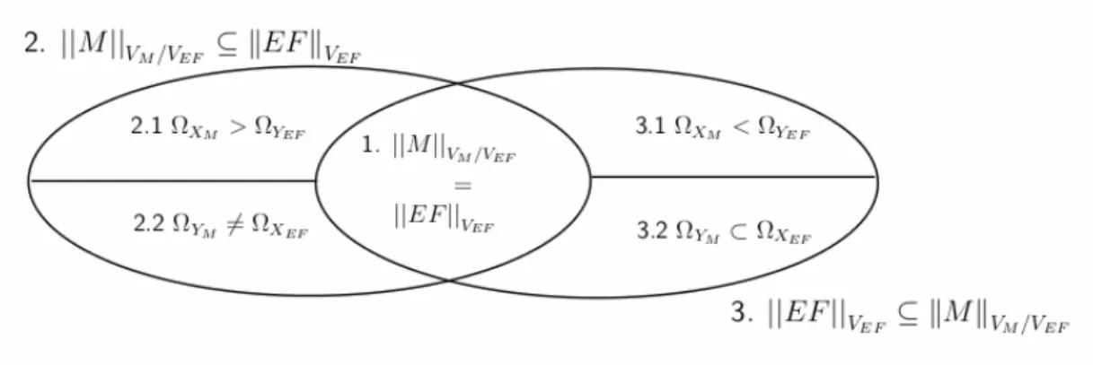
VEF (case 1 in Figure 5).Definition 11 (Relaxed compatibility).
Exact matching not being required, this means that:
•
M
VM/VEF ⊆EF
VEF : the behaviours of the model are in the envelope of significant behaviours with respect to the EF (case 2 in Fig. 5).•
EF
VEF ⊆M
VM/VEF : all experimentations planned by the EF can be performed on the model (case 3 in Fig. 5).When
M
VM/VEF ⊆EF
VEF is false, there are model executions which are not EF executions. We identify two cases (Fig. 5):• (case 2.1 in Fig. 5). There is a test coverage risk. This may be the case if the model considers input variables with other values than those planned by the EF. The EF does not therefore explore all executions of the simulation. This means that either the unexplored executions are not relevant for the experimentation, or that the EF is not comprehensive enough.
• (case 2.2 in Fig. 5). There is a bias in the simulation or in the reference definition. This may be the case as the model considers output variables with other values than those expected by the EF. This means either that the simulation results are incorrect or that the EF assumptions are false.
When
EF
VEF ⊆M
VM/VEF is false, executions are envisaged by the EF but are not model executions. Here again, two cases can be considered (Figure. 5):• (case 3.1 in Figure. 5). Some experiments are outside the usage domain of the simulation model. This may be the case if the EF considers output variables with more values than those accepted by the model. The EF therefore plans to explore simulation executions outside the scope recommended by the model and the simulation results can no longer be guaranteed. The model or EF must be modified.
• (case 3.2 in Figure. 5).There is a risk concerning the completeness of the model. This may be the case if the EF considers the input variables with more values than those supplied by the simulation results. Thus, either there is something to be learnt from the simulation if we reduce the uncertainties of the EF, or the simulation overlooks the implementation of some cases. Figure 5 below illustrates these four cases.
Figure 5. Level of EF/Model behavioural compatibility
5. Computing compatibility
A key step in our methodology is to ensure that a model provides meaningful input and output ports for a given experimental frame, i.e. a set of stimulation and observation points [22]. In other words, we focus on the boundaries between the model and the experimental frame. Thus, we can clearly perceive what drives the model, what is observed as its output, and the model itself. It is worth noting that incorporating data-gathering facilities into the model must be avoided, since this would make the model not only more complex but also unsuitable for reuse or for association with different experimental frames.
D.S. Weld [2] defines the scope of a model as the range of the system the model describes. A model has a larger scope than another if it gives a broader description of the system. Changing the scope of a model is equivalent to redefining the boundaries between the system (described by the model) and its environment. So, selecting the scope of the model implicitly includes selecting the exogenous parameters and determining their values.
Then consider a system A which has a set of endogenous parameters and a set of exogenous parameters. By reducing the scope of the model of system A, we get a system B with a new (smaller) set of endogenous parameters and a new (larger) set of exogenous parameters. The new exogenous parameters then become parameters that can be controlled and/or observed by the simulation user to properly carry out his/her experimentation. They now belong to the experimental frame. New boundaries between the experimental frame and the model of the system of interest are defined. We thus define the scope of a simulation by the set of exogenous parameters of the system of interest.
In industrial practice, a simulation is developed to verify and validate a given set of system requirements. Therefore a test plan associated with those requirements is elaborated. We assume that a test plan requiring user specification leads to an experimental frame component annotated with specific constraints, i.e. a signature. We equally assume that the component model of that system is annotated with those constraints. We can then analyse a set of compatibility properties between the experimental frame and the model. There exist static and dynamic properties. Hence simple properties (scope, values, domain...) have been found to be correct and the modeler can therefore go further to include more complex properties (e.g. a minimum user specification is required for static properties). An incorrect property informs us that the simulation cannot be executed in the given situation, i.e. either the model or the experimental frame must be modified.
5.1. Steps of compatibility computation
A component-based approach is proposed to describe a simulation. We assume that an experimental frame and a system model of interest are two components as defined by [23]. A component features a set of ports and is coupled to another component through connectors via their respective ports. A component can either be coupled, i.e. it is the result of a composition of components, or it is atomic, i.e. it cannot be decomposed any further.
Then we assume that both the experimental frame and the model are specified and can be built using a component-based approach. The experimental frame successively affects values to the model inputs (generator), triggers events and observes the model outputs (transducer). Temporal logic may be used to specify the acceptor, i.e. a set of relationships between inputs and outputs within the frame.
Consider two components EF and M defined by two IOAs : EF = 〈DEF, XEF, YEF, domEF, SEF, σEF, ΣEF, δEF, S0EF〉 and M = 〈DM, XM, YM, domM, SM, σM, ΣM, δM, S0M〉.
Computing the compatibility of the experimental frame relative to a model involves several steps: •••• Step 1: Verifying scope compatibility
The ports of a component are defined by its automaton vocabulary (X, Y and S). Then an EF and M can be connected if (definition 9): XEF ⊆ YM, YEF =XM, ΣEF ⊆ΣM.
•••• Step 2: Computing the targeted state
A simulation achieves its intended purpose if the set of summary mappings given by the acceptor are satisfied by the interaction of the model with the generator and the transducer. Remember that a summary mapping can be seen as a set of constraints which links a configuration σ(v) with v ∈ SEF and a transition l ∈δEF. v is a targeted state of the acceptor. We
denote the set of targeted states given by the acceptor by Sacc ⊆ SEF.
This step consists in verifying that for all targeted states there exists a state in the model such that:
•••• Step 3: Computing the synchronous product of the generator, transducer and model.
The generator, transducer and model share a set of events to satisfy the properties expected by the acceptor. The product allows an IOA to be built up from two IOAs. The synchronous product A of EF and M, denoted A = EF
M
is defined by:(SEF ×SM, ΣEF ∪ ΣM, δEF ×δM, S0EF × S0M) where – SEF ×SM is the set of states,
– ΣEF ∪ΣM is the set of event names,
– S0EF × S0M is the set of initial states,
– δEF×δM is the transition relation defined by:
* ((v;u), l, (v', u')) (v, l, v') ∈ δEF ∧ (u, l, u') ∈ δM ∧ l ∈ ΣEF ∩ΣM
* ((v;u), l, (v', u)) (v, l, v') ∈δEF ∧ u ∈ SM ∧ l ∈ ΣEF \ ΣM
* ((v;u), l, (v, u')) (u, l, u') ∈δM ∧ v ∈ SEF ∧ l ∈ ΣEF \ ΣM
•••• Step 4:
Verifying that EF
M
satisfies the set of properties P expected the acceptor: EFM
= P.•••• Step 5: Computing the IOA of the model restricted to the IOA of the experimental frame
(definitions 7 and 8).
•••• Step 6: Comparing execution traces (definition 12).
5.2. How to use trace inclusion
Using trace inclusion consists of evaluating a simulation based on the experimental frame approach and the steps of compatibility computation as shown in figure 6.
We assume that an evaluation of simulation is defined by the model of the system under test and de requirements to evaluate. We recall that our approach is model-based. Therefore the modeling of the experimental frame is built from the simulation requirements to obtain the following models: generator, transducer and acceptor as seen in Figure 6. Each used model in this approach has to be formally checked. It is worth remembering that an experimental frame successively affects values to the model inputs (generator), triggers events and observes the model’s outputs (transducer).
As mentioned in related work, errors not detected by formal verification are due to incorrect specifications or misinterpretation of specifications. In our approach specifications are taken into account and modeled as IOA that leads to test generation. The IOA can be checked by model checking to ensure its correctness in relation to specification and to detect different kinds of errors such as misinterpretation.
For the compatibility computation we assume the above mentioned models are formally checked and available. Compatibility can be splitted in type of metrics:
• Step 1: allows computation of scope metrics between the EF (i.e. its models) and the model under test. Scope metrics identify expected and required input/output ports of the model and the EF, respectively. These metrics are computed using the IOA of connected models.
• Steps 2 and 3: lead to the computation the compatibility metrics between model, generator and transducer thanks to synchronous product of IOA. Compatibility metrics are achieved by synchronous product between EF models and model under test to identify the applicability of event sequences between EF and model and verify the reachability of searched states given by the acceptor.
• Steps 4, 5 and 6: help to compute the coverage metrics. Coverage analysis is performed by the acceptor which provides acceptance criteria for trace inclusion. This analysis is based on the results of a verification tool as UPAAL. We compare the set of model traces, which meets the properties given by the acceptor, with the set of traces given by the generator and the transducer. With the trace inclusion approach, we can identify a priori (before simulation execution) whether a simulation can be executed indicating to the modeler whether the guarantees provided by the model will satisfy its simulation objectives of use. Coverage metrics can be defined using five quantities (figure 5): exact matching (case 1), test coverage risk (case 2.1), bias in the simulation (case 2.2), wrong usage of the model (case 3.1), and model completeness risk (case 3.2).
6. An example: Adaptive cruise controller
Our approach can be illustrated with the design of an embedded system, the control unit of an autonomous intelligent cruise controller (AICC) [24, 7]. The AICC is more than just a regular cruise controller which maintains speed as required by a driver, it adapts it according to the distance and speed of the vehicle in front. A safe speed is the maximum speed required to maintain the vehicle safely away from the other vehicles in front of the vehicle. The expected speed is the one requested by the driver. The control unit must keep the speed within ±2km/h of the safe speed or expected speed, whichever is lower.
6.1. Adaptive cruise controller simulation
The structural definition of the simulation is given in Figure 7 below. Remember that it is an important step since it allows to define the boundaries between the model and the experimental frame. Selecting the scope of the model implicitly includes selecting exogenous parameters. All other components of the global system (e.g. AICC vehicle) now belong to the experimental frame needed to represent the environment of the cruise controller. Some of these elements can be abstracted or simplified if their contributions are not relevant to the experiment.
The system of interest consists of the cruise controller calculation module which computes a throttle setting according to data from the driver and sensors. Those data include brake command, coast and acc controls to respectively decrease and increase the required speed. The safe speed and actual speed are retrieved from speed sensors.
In this context, the experimental frame consists of scenarios for brake, and required speed and a function to compute the safe speed according to the distance and speed of the leading vehicle. This is accomplished by the generator. The transducer monitors the throttle setting and updates the vehicle speed accordingly. The acceptor continually tests the run control segments to satisfy a set of constraints, e.g. the speed of the vehicle must remain within ±2km/hof the safe speed or expected speed.
Figure 7. Adaptive cruise controller simulation
6.2. Adaptive cruise controller model
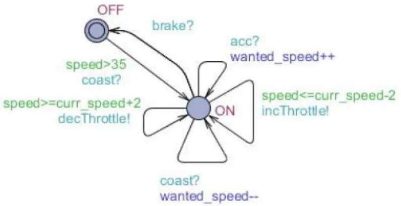
Consider a model of the AICC for which Figure 8 gives all possible executions. This model has several variables: s, ws, ss, which are the speed of the vehicle, the expected speed given by the driver, and the safe speed given by a sensor, respectively. These variables can only take the values 10 or 20. A variable status indicates whether the cruise controller is OFF or ON. A variable cs is employed to know whether the controller must maintain the safe speed or the expected speed, whichever is lower. incTh and decTh are used to adjust the throttle valve angle. The set of states S is then given by S = {status ∈ {ON, OFF}, cs ∈ {ws, ss}, ss ∈ {10, 20}, ws ∈ {10, 20}, s ∈ {10, 20}}.
The set of events is given by Σ = {acc, coast, brake, s < ws, ws ≤ ss, incDst, decDst}. When the cruise controller is OFF, if a coast event occurs, it switches to the ON state and the speed is maintained. In this state, having a coast event leads to decreasing the driver expected speed, while having an acc event results in increasing the driver’s expected speed. A brake event turns the cruise controller OFF. The s < ws event will occur when the speed (s) decreases below the wanted speed (ws). The ws ≤ ss event will occur if the wanted speed decreases to the safe speed or a speed lower than the safe speed. The incDst and decDst events respectively increase or decrease the safe speed value.
Let us now formally describe the "observable" version of the model. The state variables which are not controllable and/or observable are masked. This causes state aggregation over the model’s state space. Fig. 9 shows an abstraction of the previous reachability graph. The cs variable is hidden and the states which share the same combination of values for status, ws, s and ss are aggregated. The transition relations are kept.
Figure 9. Abstract version of the previous reachability graph
6.3. Adaptive cruise controller experimental frame
Consider then the following intended purpose: when the safe speed is lower than the expected speed, the controller must keep the speed of the vehicle at the safe speed.
There are two scenarios for which the safe speed becomes lower than the expected speed:
1. the safe speed is greater than or equal to the expected speed and an acc event increases the expected speed which becomes greater than the safe speed.
2. the safe speed is greater than or equal to the expected speed and a decDst event decreases the safe speed which becomes lower than the expected speed.
6.4. Behavioural compatibility
Given below are examples of relaxed compatibility as given in definition 11. Case 1:
Consider the model given in Figure. 9 and an experimental frame scenario which simply stimulates an acc event, then it observes ss < ws and finally s=ss.
The set of targeted states are all states where s < ss: Sacc = {s2, s5, s7}
The product EF
M
satisfies the property
ss
<
ws
→
s = ss. The algorithm used to verify that an automaton satisfies a temporal property is not given here. It can be found in [12].In the model given in Figure 9, three execution traces satisfy this property:
M
VM =1. s0
acc →
s2
ss
<
ws
→
s22. s0
incDst →
s1
acc →
s3
→
incTh
s5
decDst
→
s4
ss
<
ws
→
s4
→
decTh
s2 3. s0
acc →
s1
incDst →
s3
incTh →
s5
decDst
→
s4
ss
<
ws
→
s4
→
decTh
s2Result:
The experimental frame covers the first model’s execution trace but does not explore traces 2 and 3. This corresponds to case 2.1 in Figure 5.
There is a test coverage risk. Case 2:
Consider a model which overlooks the implementation of execution traces 2 and 3 shown above. Consider an experimental frame which stimulates a decDst event, then it observes ss < ws and finally s=ss.
The product EF
M
does not satisfy the property
ss
<
ws
→
s =ss, i.e. the event decDst of the experimental frame is not synchronizable with M. The synchronous product step failed. Therefore we don’t need to compare execution traces.Result:
The experimental frame plans to explore simulation executions are outside the scope recommended by the model. This corresponds to case 3.1 in Figure 5.
The experimental frame and model are not compatible. 6.5 Verifying trace inclusion with UPPAAL
UPPAAL is a tool environment for the modeling and verification of real-time systems modeled with timed automata. It uses Linear Temporal Logic (LTL) to encode requirements and analyse qualitative properties of models.
The behaviour of the AICC calculation module is given by the automaton in Figure 10. The second automaton in Figure 11 implements a module called UpdateSpeed used to continually check which speed must be used for cruise control, i.e. safe speed or expected speed. Observe that we have used the synchronization mechanism offered by UPPAAL to ensure that the product of the model and experimental frame satisfy the properties given by the acceptor.
Figure 10. IOA 1 of the model: calculation module
The intended purpose consists in validating the speed selection process (module UpdateData): if the safe speed is lower than the required speed, the cruise controller must maintain the speed equal to the safe speed. Otherwise, it must maintain the speed equal to the required speed. The transducer, as illustrated by the IOA Figure 12, updates the vehicle speed according to the throttle setting, and continually checks the property curr_speed == expected_speed, i.e. the cruise controller maintains the speed equal to the required speed.
Figure 11. IOA 2 of the model: UpdateSpeed
Figure 12. IOA of the transducer
Let us assign three different scenarios (Figure 13) to illustrate the different cases. We have used the UPPAAL model checker to verify the properties encoded in LTL. Figures 14, 15 and 16 show snapshots of the results.
If properties A◊ speed ≥ curr_speed-2 and A◊ speed ≤ curr_speed+2 are true, the speed of the vehicle always remains within ±2km/hof the current speed.
If the property E◊ curr_speed==expected_speed is true, there is a sequence of alternating delay transitions and action transitions where the current speed equals the required speed.
Figure 13. Left to right: generator for scenarios 1, 2 and 3
Scenario 1: ΩYM ≠ΩXEF and ΩXM < ΩYEF (Fig. 14) This scenario occurs when the execution trace of the experimental frame is not an execution trace of the model (case 3.1 in Figure 5). Some experiments lie outside the usage domain of the model, i.e. the model cannot reach the ON state from the OFF state with the event brake. Indeed, the transducer state OK will never be reached (case 2.2 in Figure 5).
Figure 14. Temporal logic verification for scenario 1
Scenario 2: ΩYM ≠ΩXEF and ΩXM >ΩYEF (Figure 15 This scenario occurs when the experimental frame does not explore all execution traces of the model (case 2.1 in Figure 5). The generator is applicable to the model, i.e. the end state is reached but does not allow to support the simulation intended purpose, i.e. the transducer state OK will never be reached (case 2.2 in Figure 5). Indeed, the left side transition of the UpdateData module is never fired.
Figure 15. Temporal logic verification for scenario 2
Scenario 3:
M
VM/VEF=EF
VEF (Figure 16) This scenario occurs when the experimental frameexecution traces are also execution traces of the model. The generator is applicable to the model, i.e. the end state is reached and the simulation intended purpose is met, i.e. there is an execution trace in which the transducer state OK will be reached.
Figure 16 Temporal logic verification for scenario 3
7. Conclusion and future work
This paper has introduced an approach to formally validate and define a context of ongoing simulation using behavioural compatibility between a model and its intended purpose. The concept of experimental frame, proposed in the M&S theory, has been employed to address the problem within a
well-founded methodological framework. It has also allowed us to treat a recurring problem in that the intended purpose of the simulation is often not well-defined. We have shown that the model is not the only cause of bias to simulation, but that the experimentation performed with this model may also have been poorly defined.
The issue of matching relies on the principle that an intended purpose and a model are two components, in the formal meaning of the term, i.e. interacting through their interfaces and only through them. We turned to component-based engineering techniques to iteratively enhance the concept of an experimental frame of "symbolic concepts" and determine the system behaviours to be included in the model.
The generator defines the logical order of the stimuli injected into the simulation. The transducer defines the logical order of the observations. We specified these two components using input/output automata. The acceptor, specified using temporal logic, consists in verifying whether a requirement has been verified based on stimulus/observation pairs. As for properties related to the applicability check between the experimental frame and the model, we also defined temporal logic properties for EF states to determine which applicability case we found ourselves in. While this approach is consistent, an effort remains to be made to find more systematic applicability properties. We have defined and compute three types of metrics: scope metrics between the EF and the model, compatibility metrics and coverage metrics within the state space. Furthermore, with this approach, coverage analysis can be performed either from scratch with the development of a simulation necessary and sufficient to satisfy an intended purpose, or with the reuse of an already existing simulation model to satisfy an intended purpose. Developers are free to associate a model with different experimental frames, each corresponding to a particular simulation objective of use.
We have two directions for the future work:
• we would refine coverage quantities and explore other gauges for metrics.The latter are ordered, i.e. measuring trace inclusion implies that ports and event sequences are compatible, • we would like to focus on establishing equivalence classes between execution traces, e.g.
traces that rise to the same conclusion can be aggregated. This would allow to reduce the number of simulation scenarios and to avoid the duplication of tests.
[1] F. K. Frantz, A taxonomy of model abstraction techniques,in: WSC ’95: Proceedings of the 27th conference on Winter simulation, IEEE Computer Society,Washington, DC, USA, 1995, pp. 1413– 1420.
[2] D. S. Weld, Reasoning about model accuracy, Artif. Intell.56 (2-3) (1992) pp. 255–300. [3] V. Albert, Simulation validity assessment, in: PhD Thesis, 2009.
[4] B. P. Zeigler, H. Praehofer, T. G. Kim, Theory of Modeling and Simulation, Academic Press, San Diego, California, USA, 2000.
[5] R. G. Sargent, Verification and validation of simulation models, in: WSC ’05: Proceedings of the 37th conference on Winter simulation, Winter Simulation Conference, 2005, pp. 130–143.
[6] D. Brade, Vv&a ii: enhancing modeling and simulation accreditation by structuring verification and validationresults, in: WSC ’00: Proceedings of the 32nd conference on Winter simulation, Society for Computer Simulation International, San Diego, CA, USA, 2000, pp.840–848.
[7] S. Schulz, J.W. Rozenblit, K. Buchenrieder, Towards an application of model-based codesign: An autonomous, intelligent cruise controller, in: Proceedings of the 1997 IEEE Conference and Workshop on Engineering of Computer Based Systems, 1997, pp. 73–80.
[8] M. K. Traoré, A. Muzy, Capturing the dual relationship between simulation models and their context, Simulation Modeling Practice and Theory 14 (2) (2006) pp. 126–142.
[9] B. Bonte, R. Duboz, G. Quesnel, J. Muller, Recursive simulation and experimental frame for multiscale simulation, Proceedings of the 2009 Summer Computer Simulation Conference (2009) pp. 164–172.
[10] S. Kops, H. Vangheluwe, F. Claeys, F. Coen, P. Vanrolleghem,Z. Yuan, G. Vansteenkiste, The process of model building and simulation of ill-defined systems: Application to wastewater treatment, Mathematical and Computer Modeling of Dynamical Systems (1999) pp. 29–35. [11] E. Lee, Y. Xiong, Behavioural types for component based design, Technical Memorandum
UCB/ERLM02/29.
[12] L. Alfaro, T. A. Henzinger, Interface automata, in: Proceedings of the Ninth Annual Symposium on Foundations of Software Engineering (FSE), ACM, Press, (2001) pp. 109–120.
[13] E. Filiot, N. Jin, J.-F. Raskin, An antichain algorithm for ltl realizability, in: CAV, (2009) pp. 263– 277.
[14] R. Alur, L. Fix, T. A. Henzinger, Event-clock automata: A determinizable class of timed automata, Theoretical Computer Science 211 (1999) pp. 1–13.
[15] B. Di Giampaolo, G. Geeraerts, J.-F. Raskin, N. Sznajder, Safraless procedures for timed specifications, in:Springer (Ed.), Proceedings of FORMATS 2010, 8th International Conference on Formal Modeling and Analysis of Timed Systems, Lecture Notes in Computer Science (2010). [16] G. Behrmann, A. David, K. G. Larsen, A tutorial on UPPAAL, in: M. Bernardo, F. Corradini (Eds.),
Forma lMethods for the Design of Real-Time Systems: 4th International School on Formal Methods for the Design of Computer, Communication, and Software Systems,SFM-RT 2004, no. 3185 in LNCS, Springer–Verlag, (2004) pp. 200–236.
[17] F. Cavaliere, F. Mari, I. Melatti, G. Minei, I. Salvo, E. Tronci, G. Verzino, and Y. Yushtein. Model Checking Satellite Operational Procedures. In DAta Systems In Aerospace (DASIA), Org. EuroSpace, Canadian Space Agency, CNES, ESA, EUMETSAT. San Anton, Malta, EuroSpace, (2011).
[18] D. L. Dill, S. Tasiran, Formal verification meets simulation (embedded tutorial) (abstract only), in: Proceedings of the 1999 IEEE/ACM international conferenceon Computer-aided design, ICCAD ’99, IEEEPress, Piscataway, NJ, USA, (1999) pp. 221–, chairman-Sentovich, Ellen M.
[19] S. Tasiran, A functional validation technique: Biased random simulation guided by observability-based coverage, in: Proc. of the 2001 IEEE Int. Conference on Computer Design: VLSI in Computers & Processors ICCD, (2001) pp. 82–88.
[20] D. Karlson, P. Eles, Z. Peng, Validation of embedded systems using formal method aided simulation, in: Proceedings of the 8th Euromicro Conference on Digital System Design, DSD ’05, IEEE Computer Society, Washington, DC, USA, (2005) pp. 196–201.
[21] J. E. Hopcroft, R. Motwani, J. D. Ullman, Introduction to Automata Theory, Languages, and Computation, 2ndEdition, Addison Wesley, (2000).
[22] V. Albert, A. Nketsa, Signature matching applied to simulation/frame duality, The Fourth International Conference on Systems (ICONS 2009) pp. 190–196.
[23] C. Szyperski, Component Software: Beyond Object-Oriented Programming, Addison-Wesley Longman Publishing Co., Inc., Boston, MA, USA, (2002).
[24] U. Palmquist, Intelligent cruise control and roadside information, IEEE Micro 13 (1) (1993) 20–28. [25] T. Mancini, F.Mari, A. Massini, I. Melati, E. Tronci, System level formal verification via model checking driven simulation. In Proceedings of the 25th International conference on computer aided verification pp 269-312, (2013) Saint Petersburg Russia.