The integer transfinite diameter of intervals and totally real algebraic integers

J

OURNAL DE

T

HÉORIE DES

N

OMBRES DE

B

ORDEAUX

V. F

LAMMANG

G. R

HIN

C. J. S

MYTH

The integer transfinite diameter of intervals and

totally real algebraic integers

Journal de Théorie des Nombres de Bordeaux, tome

9, n

o

_{1 (1997),}

p. 137-168

<http://www.numdam.org/item?id=JTNB_1997__9_1_137_0>

© Université Bordeaux 1, 1997, tous droits réservés.

L’accès aux archives de la revue « Journal de Théorie des Nombres de Bordeaux » (http://jtnb.cedram.org/) implique l’accord avec les condi-tions générales d’utilisation (http://www.numdam.org/conditions). Toute uti-lisation commerciale ou impression systématique est constitutive d’une infraction pénale. Toute copie ou impression de ce fichier doit conte-nir la présente mention de copyright.

Article numérisé dans le cadre du programme Numérisation de documents anciens mathématiques

The

_integer

transfinite diameter of intervals and

_totally

real

_{algebraic integers}

par V.

FLAMMANG,

G. RHIN et C.J. SMYTH

RESUME. Dans cet _article, nous _inspirant de travaux récents d’Amoroso d’une part, de Borwein et _Erdélyi d’autre _part, nous donnons une

ma-joration et une minoration du diamètre transfini entier de petits inter-valles +

_03B4]

est un rationnel fixé et 03B4 tend vers 0. Nous étudions _également des fonctions _{g-, g,}

_g+

associées au diamètre

trans-fini d’intervalles de _Farey.

Nous introduisons ensuite la notion de polynômes critiques pour un in-tervalle I. Nous montrons que ces _polynômes ont la propriété de diviser

tout _polynôme à coefficients entiers ayant un maximum suffisamment _petit

sur I. Aparicio, puis Borwein et _Erdélyi ont obtenu des résultats _pour le

polynôme critique x sur l’intervalle _{[0,1] ;} résultats que nous prolongeons à

tout _{polynôme critique} sur un intervalle arbitraire.

Par _ailleurs, comme _conséquence facile de nos résultats, nous montrons :

si 03B1 est une entier _algébrique totalement _réel, de _{plus petit conjugué} 03B11 alors, sauf pour un petit nombre d’exceptions explicites, la valeur _moyenne

de 03B1 et de ses _conjugués est _supérieure à 03B11 + 1.6.

ABSTRACT. In this paper we build on some recent work of Amoroso, and Borwein and _Erdélyi to derive _upper and lower estimates for the integer

transfinite diameter of small intervals +

_03B4],

is a fixed rational

and 03B4 ~ 0. We also study functions _{g-, g,}

g+

associated with transfinite

diameters of Farey intervals. Then we consider certain polynomials, which we call critical polynomials, associated to a _given interval I. We show how to estimate from below the _proportion of roots of an _{integer polynomial}

which is sufficiently small on I which must also be roots of the critical

polynomial. This _generalises now classical work of Aparicio, and extends the _techniques of Borwein and _Erdélyi from the critical _{polynomial x} for

[0,1]

to any critical polynomial for an arbitrary interval.

As an _{easy consequence} of our _results, we obtain an _inequality about

algebraic integers of _independent interest: if 03B1 is _{totally real,} with minimum

conjugate 03B11, then, with a small number of explicit exceptions, the mean

value of 03B1 and its _conjugates is at least 03B11 + 1.6.

1. Introduction. For a set I in the

_{complex plane,}

its

transfinite

diameter

_t(I)

is

_{given by}

i.e. the

_limit,

as n tends to

_infinity,

of the _supremum of

_geometric

means of the distances between n

points

in I. This has been

computed

for _many

sets I. For a real interval I of

_length

_III

it is

_111/4.

Fekete

_[Fek]

_(see

also

[Gol])

showed that an

_equivalent

definition of

t(I)

is

where the infimum is taken over all non-constant monic

_polynomials

P

Further,

if I is a real _set, then this infimum can be restricted

to

_polynomials

in

_Clearly

"monic" could be

_{replaced by}

_"leading

coefficient at least 1" in

_(1.2).

If I is a real

_set,

and the coefficients of P are restricted to be

_integers,we

can define

the

_integer

_transfinite

diameter

_of

I. It is known that

the first

_{inequality being}

_immediate,

the second a classical result of

_Fekete,

readily

deduced from the discussion on

_pp.246-248

of

[Fek].

While the classical transfinite diameter

_{t(I )}

is

_{translation-invariant,}

scales

_linearly

and is therefore additive for

_abutting

_intervals,

none of these

_properties

holds in

_general

for

_(see

_Corollary

_(4.3)).

For intervals I of

_length

at least

_4,

it is known that

_{_ ~ I ~ /4,}

([Gol],p.298),

so we restrict our attention to

_studying

_tz(I)

for smaller intervals. From

_(1.4),

1 for all such intervals.

_Recently

Borwein and

_Erd6lyi

_[BoEr]

_pointed

out a connection between

_finding

_polynomials

in whose maximum is small on

[o,1],

and

_{finding degree}

d real

_algebraic

integers

of norm

_N,

all of whose

_conjugates

lie in

[l, oo),

for which is small. Their fruitful idea

_provided

the stimulus for this _paper. It has also been

_applied

in

_[F12],

where it is used to obtain

_good

_upper and lower bounds for for _many sub-intervals

Essentially,

the idea is to use a fractional linear transformation to _map

certain families of

_{totally positive}

_algebraic

_integers

to families of

_algebraic

numbers with all

_conjugates

in I. For I =

[o,1]

itself,

the result

_given

there is the same lower bound as one due to

_{Aparicio[Apl],}

and is indeed

equivalent

to it

_([F12]).

It was

_{long suspected}

(see

_e.g.

Chudnovsky[Chu])

that this classical lower bound in fact was the true value of

_{tz (I) .}

_However,

Borwein and

_Erd6lyi

_[BoEr]

_show,

_very

_{surprisingly,}

that this is not the

case. Thus to date no-one has been able to

_compute

_{tz (I)}

_exactly

for _any

interval of

_length

less than

_4,

and there is now not even a

_conjectured

value for

_it,

for any such interval I!

For an

’integer Chebyshev’ polynomial

for

[0, 1] ,

i.e. a

_polynomial

with

integer

coefficients whose maximum among

polynomials

of a fixed

_degree

is

minimal,

Borwein and

_Erd6lyi

_[BoEr],

_p. 679 asked whether it must have all its zeroes in

[0, 1].

Recently Habsieger

and

Salvy[HaSa]

showed that it need

_not,

_by

_finding

that the

_degree

70

_{integer Chebyshev polynomial}

for

[0, 1]

had a factor with four non-real zeroes.

There have been some

_applications

of estimates for

_{tz (I)}

for intervals. For

_instance,

Schnirelman and Gelfond

_(see

_{Ferguson[Fer]}

_p143)

_give

a beautiful and short

_elementary

_argument

_proving

that

for the

_{prime-counting}

function

_Also,

an _upper bound for

y’m)2])

(n, m

positive

integers)

gives

an

_{irrationality}

measure for

_log(n/m)

_([Rh1]).

In Section 2 we introduce a

_{(presumably transcendental)}

function

_g-(t)

associated to a

_family

of

_totally

real

_algebraic

_integers.

This function

en-ables us to

_give

a lower bound for for all intervals I of the

_type

_(1.5).

In Section 3 we

_study

a function

g(t),closely

associated to show that

_{g_}

_g, and find other bounds for _g.

In Section 4 we consider for _{very small}

_intervals,

i.e. for intervals I where we let the

_length

~I~

tend to 0. Here we

generalise

and sometimes

improve

results of Borwein and

_Erd6lyi

_[BoEr]

and

_Amoroso[Am]

on this

topic.

(See

also

_[La]).

_(Amoroso’s

_techniques

_are,

_{however, quite}

different

the

2- norm J fIr II 1P12,

and works with this

_instead.)

These results show how _very different in relative size

_tz(I)

can

_be,

for different intervals of the same

length 6 ,

as 6 -~ _0. We also

_show,

_using

a nested _sequence of

Farey

intervals,

that can be as

_big

as

0.420726..B/)TJ~

so that the constant

~

in

_(1.4)

cannot be reduced

_by

much.

In Section

_5,

we introduce the notion of critical

_polynomials

for an in-terval I. These

_polynomials

have the

_property

that

_they

must _{divide any}

integer-co efficient

polynomial

P which has a

_sufficiently

small maximum on the interval. We _prove

_(extending

results of

_{Aparicio[Ap3]}

and of Borwein and

_Erd6lyi

_[BoEr])

that not

_only

must critical

_{polynomials Q}

divide the

polynomial

P,

but that there is a

positive

constant 1

independent

of

P such that As an

_application,

these

_{constants y}

are

_computed

in

Section 6 for all ten known critical

_polynomials

of

_(0,1J.

Finally,

in Section

_7,

we _prove the

following

result of

_independent

inter-est,

which follows

_easily

from a result

(Proposition

7.1)

which we need for the results of Section 4.

THEOREM 1.1. Let a be a

totally

real

_algebraic

_integer

of

_degree

8a with least

_conjugate

al. Then

unless,

for some rational

_{integer k,}

a + k is a zero of one of the

_polynomials

given

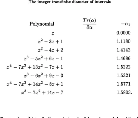
in Table l.

We also list

_{(Table 6)}

all

_polynomials

of

_degree

_up to 6 with

_Trace/degree

-al less than 1.7.

2. The function _g-, and a lower bound for

_Firstly,

we define two families

_{Uk}

and

_{Vk}

of

polynomials,

all of whose zeroes

lie on the

_imaginary

axis. These are the

_polynomials

such that is the kth iterate of the function

_G(z)

:= z +

_1/z.

_They

are

_closely

related to the Gor0161kov

_{polynomialsGor.}

_(See

the

_Appendix

for the

_precise

connec-tion,

for a _{summary of}

_properties

of Gorskov

_polynomials,

and for related

references.)

The

Uk

and

Vk

are defined

inductively by

_Uo

= _z,

Vo

= 1 and

TABLE 1. List of all monic irreducible

_polynomials

with all

roots

_real,

least root in

_[o,1),

and

_{(Trace/Degree) -}

al at most

1.6.

for k &#x3E; 0. Note that

_aUk

=

2k,

=

2k -1. If

we

_put

_x~ := then

Also,

it is known that

_Uk

and

_{Vk ,}

or

_U~

and

_Uk,

with k

k’

have no com-mon _zero, and that

_Uk

is irreducible

(See Appendix).

The Julia set of the map

G(z)

is the

imaginary

axis

J,

and the

(Lyubich)

invariant measure 1L is defined as the weak

_limit,

as k - o0 of the atomic

probability

measure

having

equal weights

at the zeroes of

_{Uk .}

_(See

[St],

_p164,

and the

Appen-dix).

[Here

invariance means that =

A(E)

for

every Borel set E C

_J.]

This measure

_gives

rise to the

_logarithmic

_potential

which is a harmonic function on

CBJ

(see

[St],

p17).

In

fact,

as

~(z-x)

&#x3E; 0 for Rz &#x3E;

_{0, x}

E

_J,

the

_{’complex potential’}

(taking

the

_principal

value of

_log)

is

_readily

shown to be

_analytic

in the

right half-plane

Rz &#x3E; 0. We now define a function

_{g_ (z)}

for z in this

half-plane by

Then we claim

LEMMA 2.1. On the

_half-plane

Rz &#x3E; 0 the function g- is

analytic,

is

given

by

and satisfies the functional

_equations

and

.Furth erm ore,

for

_{real, positive}

t we h ave th e bounds

and hence

_certainly

as _xo = z.

_Convergence

of this

product

can be verified

directly

from the fact that

_Rxk+l

&#x3E;

RXk

and

_S’Xk.

_Equation

_(2.5)

now follows

straight

from the fact that

_xl(z).

To prove

(2.6),

note

that,

from

_(2.4),

which

_gives

the result.

Now take z = _{t &#x3E;} 0. To _prove

(2.7),

first note

that,

from

(2.4),

We now claim that

This is

_readily

verified

_{by induction, using}

xk+1= xk +

x. 1 -

Hence

which

_gives

the left-hand

_inequality.

For the

_{right-hand inequality,}

use the fact that txl = 1 +

t2.

Another functional

_equation

follows

_straight

from the

_lemma,

from which it is easy to

_produce

the

as-ymptotic

series

The

_graph

of g- is shown in

Fig.

1. Its maximum value is

g-(1) =

0.420726377.

With the aid of the function g- we can reformulate a result in

_[F12]

(Theorem

1.2. See also

_[F13]):

PROPOSITION 2.2..For a sub-interval I =

[~,;]

of

_[0,1~

with _{qr - ps} = 1

Fig.

1. The function _g- and some

computed

values of

g+ .

We now use this result to show

COROLLARY 2.3. Given a

_positive

irrational

number v,

there are

_arbitrarily

small intervals I

_containing

v which have

are the

_convergents

in the continued fraction

_expansion

of v. The

_proof

is

_immediate,

from the consideration of the

_Farey

intervals with

_endpoints

- _and

qn

·

C O RO L L A RY 2 . 4 . Th ere are

_{arbi traril y}

sh ort in t ervals I for which, th e

0.420726377 ....

_Further,

in _any

_inequality

_(c,

a &#x3E;

₀₎

valid for

_sufficiently

short intervals

_I,

we have a

:5 ~.

Proof. Let v be

_{given by}

the continued fraction

_{~l, 2,1,3,1,4,1,5, ].Then,}

from the recurrence for

the qn ,

it follows that 1. The

qn+l

second

_part

follows

_immediately.

3. The function g, and upper bounds for t7l. It is convenient to

work here with

_degree

d

_{polynomial-powers,}

which we define to be expres-sions of the

_type

.

-for some

_polynomial

P (x)

E

_7G[x],

of

_degree

9P,

and d =: 8X a

_non-negative

real number.

_(While

the

_phase

of X is not

_{well-defined,}

_{~X ~ is,}

which is all we

need.)

Then

_by

definition

To define the

_g-function,

we first define a function _gp as follows: fix a finite set P = of

polynomials,

and A = a

_{corresponding}

set of

_non-negative

real

_numbers,

and

_put

a

_{polynomial-power}

of

_{degree d}

= 2:

_Aj.

Then _gp is defined for t &#x3E; 0

_by

of

_degree

_d,

where 0 d 1.

_(The

search for an

_{optimal A}

is a

problem

in "semi-infinite

_{LP" ,}

and can be carried out

_by,

for

_instance,

the Remez

algorithm

[Ce]).

Thus

_{gp (t)}

is the least number such

_that,

for some

I - I

Next,

put

LEMMA 3.1. For _{qr - ps} = 1 _we have

Proof. We

have,

for

_Xx

as defined

_above,

on

_putting

and

a

_degree

d

polynomial-power

in t. Since is a

_general

_degree

1

_{polynomial-power,}

we have the result.

COROLLARY 3.2. We have

for _any set P of

_polynomials.

Informally,

we can define a function

g+(t)

by

_choosing,

for a

_{given t,}

a

set

_Pt

of

_polynomials

_{for which gp,}

_(t)

is

_small,

and

_putting

_g+

_(t)

:= _gpl

(t).

Then

Some values of such a

g+

are shown in

_Fig.

_1,

_using

_computations

from

[F12].

PROPOSITION 3.3. For

_0,

Proof. The

_proof

is in essence the same as that of the classical lower

bound for

_{tz ([0, 1]),}

which is

_equivalent

to the

_inequality

_g(1)

&#x3E;

_{g- (1) -}

We

note first that for al, ... , ad a

complete

set of

_{conjugate positive}

_algebraic

integers

-so that

for :f:..j-ai

the zeroes of

_Pk,

and k

_{large enough}

so that no _power of

_Pk

divides Xx. The result follows on

_{letting k}

2013~ oo.

From

_[BoEr],

Theorem

_3.4,

we now

know,

surprisingly,

that &#x3E;

g_ (1),

so that

_{g- #}

_g.

_Presumably

Borwein and

_Erd6lyi’s

method will extend to show that

_g(t)

&#x3E;

_{g- (t)}

for t &#x3E; 0.

Next,

we derive a functional

equation

and a functional

inequality

for _g: PROPOSITION 3.4. The

_{function g}

satisfies for all t &#x3E; 0

[Compare

Lemma

where P* = · Since every set of

polynomials

belongs

to a set with P =

P*,

we have

and

_(3.11)

follows.

To _prove

_(3.12)

note first

_that,

for _any set P

Now,

for _any

_polynomial

_P,

for some

_{reciprocal polynomial}

_R(x)

=

x2aPR

(~),

so that

Thus,

on

defining

as

_8Rj

=

28P~,

for

X’

a

_{polynomial-power, again}

of

_degree

So from

_(3.13)

as

(t

+ +

t ) &#x3E;_ t2

for t 1. Then the lower bound follows on

_using

(3.4).

For the _upper

bound,

note that

as both minima are attained at the same A. Now for

_{any P3}

where

_{Q =}

_Finally,

from the definition

_{of g}

and the fact that

_{gQ &#x3E; g,}

we obtain the _upper bound

for g

(t

+ t~

in

(3.12).

4. Small intervals with one rational

endpoint.

In this section we bound for small intervals of

_{length 6}

with one fixed rational

endpoint

9 .

Our main result is the

_following:

THEOREM 4.1. There is a

_numerically

determined constant c and a func-tion

_{m(b) (0}

b

₁₎

for which the

_following

estimates hold. Let c &#x3E; 0 be

arbitrary,

r/s

be a rational numberin

(0,1]~

and let 6 min

(llc,

2c/c 2 )/S 2

Let

_p/q

be the

_Farey

fraction of

_largest

denominator with

and put

where ~ ~

denotes fractional

_part.

Then the interval

_{[~ 2013}

_6,

_~]

has

_integer

transfinite diameter in _{the range}

the _upper bound

_being

attained at b = 0 and 1.

further,

if b =

0,

then the

left-hand side of

_(4.1)

can be

_replaced

_by

8s -

28283.

The constant c is that in

Proposition

7.1. The theorem

generalises

results of

_[Am]

and

_[BoEr]

for s = 1.

_However,

for the upper

bound,

Amoroso had

the better constant 1.648 instead of our 1.6-e above

_(in

the worst

_case).

We

expect

that we should be able to

_improve

the constant 1.6 in

_Proposition

7.1 to

_greater

than

_1.65,

with a

_{corresponding}

_improvement

here.

_(See

the remarks after the

_proof

of

_Prop.

_7.1).

For the lower

_bound,

Amoroso

already

had the above bound

_{(I.e. 6 -}

_2b2)

in the case s =

1, b

=

_0,

while

Borwein and

_Erd6lyi

showed that the 2 could be

_replaced

_by

a number less than 2.

COROLLARY 4.2. The same bounds

~0,1), 0

l5 1 - r_s.

Proof of 4.2. This follows from the fact that

_{tz ( [a, b])}

=

b,1-

a )

for

0 a b

1,

which in turn comes from

replacing x by

1 - ~ in a

_"good"

polynomial P(x)

on

[a, b].

The

_following

result is well-known:

COROLLARY 4.3. None of the

_{putative properties}

_{tz (ci) =}

or +

_c)

= holds in

general.

Proof of 4.3. For

counterexamples

to the first

two,

note that

using

Theorem

_2.2,

while

_{t~ ( (0, 2~ ) ~}

_by

_{(1.4) .}

For the

_third,

note

_that,

from Theorem

_4.1,

for 6

_sufficiently

small.

See also Rhin

_[Rh2]

for another

_example

of this kind. For the

_proof

of Theorem

_4.1,

we need the

following

LEMMA 4.4. For 0 A

_6,

b E

_[0,1)

and x &#x3E; b we have

Proof It is

_readily

checked that has minimum value v in

_{[b, oo)}

of

shows that

Proof of Theorem 4.I. The basis of the

_proof

is the use of two

Farey

intervals

[~-, ~]

and

[~7,

_{s ~}

with

For our

_given

_{rational 1:,}

we choose the rational P-

_1:

to be the

_adjacent

.9

. ’7

s

rational in the

_Farey

series of

_largest

denominator s. Thus qr - ps = 1.

Then also ,,~

Choose k so that

Then for

_p’

_{:= p+kr}

_(and,

for later use,

p"

:=

p+(k+1)r)

and a :=

r / s - 6

so that b E

_[0,1).

Note also that

Now suppose that we have found a

_positive

function

ml (b) (0

b

1)

such

_that,

for each b there is a

_{polynomial-power}

_Ub

of

_degree

d* with

Note that d*

_1,

as otherwise the left-hand side of

_(4.6)

would be

_negative

for

_large

~.

_Then,

in a similar way to

_(4.1-2),

where

is of

_degree

d* in t. Thus the left-hand side of

_(4.7)

is a

_degree

1

polynomial-power in

t,

showing

that

To find ml

(b)

for 6

small,

we note

_that,

from the definition of b

_above,

Next,

we use the fact

_that,

_by

_Proposition

_7.1,

we can find a constant c

and,

for each b E

_~0,1)

a constant

_m(b)

with

_{m(b) -}

b &#x3E; 1.6 such that there is a

_{polynomial-power}

Wb

with

and

Then,

for each 6 &#x3E;

_0,

and A :=

s2 S,

_using

(4.4)

and then Lemma 4.4 we have

for

_a

=:

Ao say,

i.e. 8

Hence from

(4.8)

for A

_Ao

and x &#x3E; b.

_Then,

_putting

_Ub

:=

(Wb)À

we can take

...

so that

giving

the _upper bound of

_(4.1).

For the lower

_bound,

choose

_{p" and q"}

as at the start of the

_proof.

_Next,

note

_that,

from

_(2.8),

_t"g(t")

&#x3E; t2 - 2t4

_{if .1}

&#x3E; t"

&#x3E; t.

_Now,

with the

_help

of

_(4.4)

choose t’ and t"

to be

Then,

by

Theorem

_2.2,

as t2 s2 b.

This

_completes

the

_proof

of Theorem 4.1.

5. Critical

_polynomials

and lower bounds for

_exponents.

Con-sider an irreducible

_polynomial

_{P(x) =}

_adxd

+ ... E

_Z[x],

ad &#x3E;

0,

all

of whose zeros ai lie in an interval

_I,

and for which its critical value

cp := is

_greater

than We call such a

polynomial

a critical

polynomials

(for I).

In

_practice,

of _course,

_tz(I)

is not known

_exactly,

so that in order to

_identify

a

_polynomial

P as

_being

critical for I we need to

find another

_polynomial

_Q

in

_Z[z]

whose maximum

is less than _cp, so that

Now,

by

a classical

_argument

_(see

_{[Chu], [BoEr])}

if P and

_Q

are

_relatively

prime,

and P has all its zeros in

_I,

then cp. Thus if P is critical

for I then P and

_Q

must have a non-trivial common

_factor,

so that in fact

P divides

_Q,

since P is irreducible. Note that

_then,

_writing

Q

=

PkR

_we

have that

We now show

something

_stronger

than

P~Q,

namely

that

THEOREM 5.1.

_Suppose

that the

_polynomial

P is critical for

_I,

with critical value _cp, and that

_Q

E

_Z[x]

has m := _cp. Then

Pk divides

Q,

where k &#x3E;

_{,8Q, where y}

&#x3E; 0

_{depends only}

on P and m.

The

_proof

of Theorem 5.1 follows

_straight

from

_Proposition

5.3

_below,

on

_taking

P to be critical for

_I,

and M := cp.

Specific

lower estimates for

y are also

given.

As

examples,

the lower

bounds 7

are then

computed

in Section 6 for all known critical

_polynomials

of

_[0,1~.

This result is

_essentially

a

_{generalisation}

of a result of Borwein and

Erd6lyi

[BoEr],

where

_they

prove this result in the

special

case of the critical

polynomial x

for I =

(0,1~.

The basic idea is as follows: for any _{zero a} in

I of a critical

_polynomial,

_{re-parametrize}

_{by y}

E

_{[0, 1]}

a sub-interval of I

having

a as one

endpoint.

Then

apply

their

_argument,

making

use of the

y-parametrization.

However,

we first need a

_slight

_{generalisation}

of a result of theirs

( [BoEr~,

Theorem

_3.1):

LEMMA 5.2. Let _{c, m,} M be

_positive

constants with m M.

_Suppose

that there is a real

_polynomial

where 0 k n, with

cAM’and

rra. Then k &#x3E; _yn, where _-y is the least

_positive

root of

Proof This is

_essentially

the

_{proof given}

in

_[BoEr]

for c = 1.

However,

it has been modified so that it is valid for all _n, instead of

_only

for n

sufficiently

large.

We

_apply

the Gram-Schmidt _process to the

_{inner-product}

space of real

polynomials

with ordered basis elements

_xn,

_{x’~"1, ... , xk,}

and

_{inner-product}

~p, q~

:= This

_gives

[BoEr]

the

Muntz-Legendre

polynomials

- ₊

1).

Now,

writing

= we have

j/

2 2J

+

₁

_and,

since a is the coefficient of

xk

in

AkLk ,

Next,

from the

_{simple inequality}

we

_obtain,

for a =

k/n

and

that

_{f (a)}

and hence that

Finally,

since _{any power}

_f~~

of

_Q

also satisfies the conditions of the the

lemma,

we can

_{replace n by}

nN and k

_by

and let N - _oo,

_giving

simply

from which the result follows.

PROPOSITION 5.3. Let P be a real

_polynomial

with all its zeroes ai distinct

and

_lying

in

_I,

and R another real

_polynomial

such that

for some

_{positive integer k,}

wh ere m M 1. Then there is a

_positive

independent

of R

_(but

in

_{general depending}

on

_I,

_m,

_M,

and

P)

such that I~ &#x3E; _In.

_{Explicitly, ,}

is

_{given by}

Lemma 5.2 with the constant c defined as follows:

let I =

[t_, t+], a1, ... ,

be the zeros

of P’,

and _xo :=

_{t_,}

_zap :=

t+,

while for i =

2, ... , 8P --1

let _xi be

specified by

being

the _two

roots

_ai)

=

P’(ai)

in

(ai-1,

cxi+1 ) .

Then c can be taken to be

if 9P &#x3E; 1

where

Proof From

_(i),

there is some at, say a, such that Let u be a

_point

in I such that there are no zeros of P in

[u, a)

(or

(a, u]

if u &#x3E;

_a).

Put d := u - a

_{(possibly negative),}

_Po(x)

:=

P(x)/(x - a)

and

y :=

(x -

a)/d.

Then for 0

_{y 1, x}

E I and 0. Hence

_(ii)

where n :=

8(P*’ R) .

Thus if

then

as m 1. Hence we can

_apply

Lemma 5.2 to the

_polynomial

_{y k(rd)k R(yd+}

a),

whose coefficients of

_yk

is at least in modulus. Thus we can take c := in the lemma.

In order to

_get

_good

estimates

_{for q}

for

_particular

critical

_polynomials

of a

_specific

interval

I,

we need to choose u so that the value c =

rldl

is

as

_large

as

_{possible. Working for}

us is the fact that we can choose d to be of either

_{sign, allowing}

us to choose whichever

_sign

maximises c.

_Working

against

us,

however,

is the fact that we don’t know which aj is a, so we

must minimise over all i .

To obtain a

_good

value of _c, we first assemble some

_elementary

facts about

_{P, P’,}

_{the Pi}

and their roots:

(iii)

For 9P = 1 and =

2, ... , o~P - 1,

I

has a

_unique

maximum in

and the

_equation

has

_exactly

two roots ai

and

_(say)

xi in this interval.

(iv)

For

_{each i,}

is monotonic in and in

_{[aa p, t+~.}

We now

_apply

these results to the

_proof.

The case aP = 1 is

trivial,

_so

we can assume that 8P &#x3E; 1. For each zero ai of P we

_{choose, successively}

for each

_I,

the number u above to be one of

aZ_1, a~

or _xi, as follows:

For d = u - _ai we want to choose d so that

is as

_large

as

possible.

Clearly

we need u E so that

_{wi (d) ~}

0.

Now,

by

(iii)

above,

I Pi (ai

+

_yd)

_has

no local minimum for _y E

_{[0, 1],}

and hence

Now and +

_{d )}

have the same

_sign

in _{the range} of d under

discussion,

so the maximum of occurs when

_P’(az)d

=

P(ai

₊

d)

_or

when

_P’(ai

+

_d)

= 0 _or when _{ai +} d is an

endpoint

of I

(i.e.

d =

ai_1 -

_ai

or

_{a~ -}

_az in either of these last two

_cases.)

If

_aN

_{(respectively}

_{az_1)}

is

between ai and xZ then the maximum

of wi (d)

on

[ai, aZ+1]

(respectively

lai-1, ai])

occurs at xi

(i.e.

for d = xi -

ai).

Otherwise it occurs at

(respectively

(}~-1).

The final value of c is obtained

_{by minimising}

over all i. This

_completes

the

_proof.

6.

_Application

to

_{[0, 1].}

In this section we

_apply

our results to the interval

_{[o,1] .}

To do

_this,

we make use of some

_computations

from

[Fll].

All the

_polynomials

have all their zeroes in

_{[0, too),}

_{and among such}

_polynomials)

have small absolute Mahler measure

(see [Sml]).

_Following

_{[BoEr], [F12]}

define

poly-nomials

_by

_{Qo (t)}

= _{t -} 1 and

I . I

Then,

from

_[Fll],

_{pp. 67-68} the

_{polynomial-power}

_{Q(t) _}

6t + has

_m[o,l]

_(Q)

=

0.42353115,

_so that _any

polynomial

atd

₊ ...

with all zeroes in

_(0,1~

and 0.42353115 is critical. In

_particular,

are all critical. Now

_apply

Theorem 5.1 with the

_precise

lower bound

_{for 7 given}

_by

Lemma

_5.4,

for M := _cp and m :=

m[o,l]

(Q).

We see that if a

_polynomial

P with

_integer

coefficients satisfies

then divides P. The

_{polynomials Qi,}

the

_{corresponding}

_exponents

y2 and critical values cQi are as follows:

TABLE 2. Ten critical

_polynomials

for the interval

_[0,1].

Earlier

_Aparicio

_[Ap3]

had obtained the values _1’0 -

_0.1456,~2

=

0.016 and q3 = 0.0037. Borwein and

Erd6lyi

[BoEr]

improved

1’0,1’1

sub-stantially

to 0.26.

_{Further, they}

showed

_{(Corollary 2.3)}

that these

poly-nomials

_Qi

must all be factors _{of any}

_{"integer Chebyshev}

_polynomial"

of

[0,1],

which has

_sufhciently

_high

_degree,

i.e. of _any

_polynomial

P for which

(P)

is _{minimal among all}

_{integer polynomials}

of that

_degree.

Here we

quantify

their result

_by

_providing

lower bounds for the power of the factor

Qi

dividing

P,

relative to the

_degree

of P.

7. The trace of

_totally

real

_algebraic

_integers.

The main result of this section is the

_following,

which was needed in Section 4:

PROPOSITION 7.1. There is a constant c such

_that,

_{for every b in}

_[0,1)

there is a

_{polynomial-power}

_Xb

_{such that for} x &#x3E; b

an d for x &#x3E; c

Proof.

For b =

0,

one can check

_that,

for

and all x &#x3E; 0 we have

This

_Xo(x)

was the

_{polynomial-power}

used in

_[Sm2](see

also

_[Sm3])

to

prove that 1.7719 for all

totally

positive

algebraic integers

not a zero of

Xo.

(Xo

did not _{appear in}

_[Sm2]

as the table

_containing

it was removed to save

space).

We refer to this

_computation

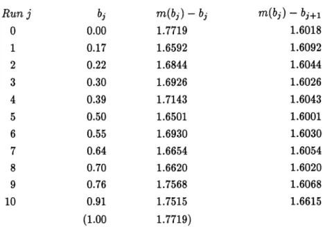
as Run 0 in Table 3. We have now

_found,

_by

a

_Remez-type

_optimisation

_algorithm,

, 10 further

polynomial-powers

_Xb~

( j

=

_{1, ... ,}

10)

where,

for b

= bj

, , ,#.-- , ,

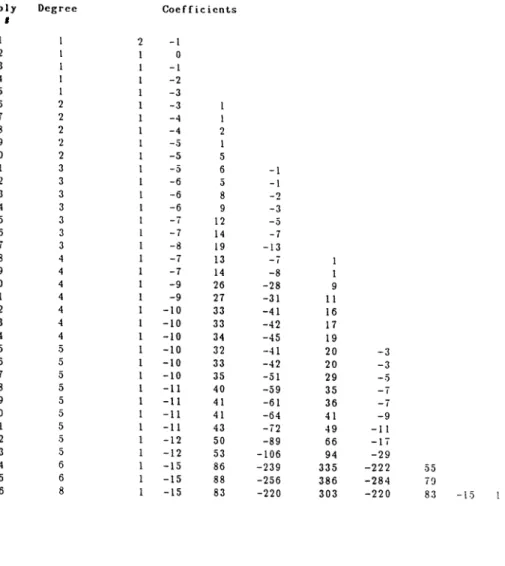
The

_{bj, m (bj)}

and

_Xb,

_Pnii

_{(x )eii}

are

_{given by}

Tables

_3,4

and 5. The

_polynomials

used in the

_{optimisation,}

and those in Table

_6,

were found

_by

the same search

procedure

as used in

_[Sm3].

_However,

the

poly-nomials searched for were

specified

to have their zeroes in the intervals

[0.05

k,

oo), (k

=

0,1...

19)

instead of

only

[0,

oo)

as in

_[Sm3].

Note that

(this being

of course the basis

_by

which the

_bj

have been

_chosen)

so that

certainly

(7.1)

holds for b =

bj.

But

also,

any

inequality

(7.3),

valid for b is also

_trivially

valid

_(with

_Xbl

:=

Xb)

for x &#x3E; b’ with

b’

&#x3E; b.

_Thus,

if we

TABLE 3. The values of b used in the

_proof

of

_Proposition

_7.1,

and

_required

functions

_{of m(b).}

(7.1)

holds for all b E

_{[0, 1).}

_Finally,

_(7.2)

is a _consequence of the fact that

Xo

above,

and each of the

_Xb’s

in Table 5 is

_{O (x2 ~83 ) ,}

As mentioned

_earlier,

we

_expect

that,

with the use of

_{substantially}

more than ten

_{values bj}

of

_b,

we should be able to

_improve

the constant 1.6

to at least

_1.65,

in Theorem

_4.1,

_Proposition

7.1 and Theorem 1.1. This is because all the values in Column 3 of Table 3 are at least this value. Of course further

_improvements

_{may also be}

_{possible perhaps using}

extra

polynomials.

One

_polynomial

_{which may}

_give

such an

improvement

is the

factor of

_Habsieger

and

_{Salvy’s polynomial}

mentioned in the introduction. The

_proof

of Theorem 1.1 now follows

_easily.

Let a and _al be as in the statement of the theorem.

_By

_replacing

a

by

a -

Laij

we can assume that

al E

[0, 1).

Then we take b = _al in

Proposition

7.1,

and _so

by

(7.1)

z

unless

_(ai)

=

_0,

_as

ITi

(ai)

is _a

_product

of

_positive

resultants of the minimal

_polynomial

of a and the

_{polynomials making}

_up Hence

_(1.6)

holds unless al is a root of one of the

_polynomials

of Table

_5,

and

_only

those listed in the statement of the theorem

_actually

have 1.6 + al.

TABLE 6. List of irreducible

_polynomials

_up to

_degree

6 with all zeroes

real,

minimum zero _rl in

[0,1],

and

trace/degree

_-rl less than 1.7000.

Appendix:

The Gorskov

_polynomials.

These

_polynomials

_Gk

were defined

_originally

_by

_{Gorgkov[Gor],}

and later

_{independently by}

_Wirsing

and

_Montgomery

_[Mo],

_p.183

and

_by

_Smyth[Sml].

See also

_[Ap2],

_p.6,

and

_[BoEr],

_p.667.

_They

are

_monic,

with

_integer

coefhcients. One could say that the Gorskov

polynomials

bear a

comparable relationship

to the

positive

half

_line,

where all their zeroes

_lie,

as the

_{cyclotomic polynomials}

do to the unit circle.

Let Hz

_{:= z - 1 /z,}

and let H kz be its kth iterate. Put

_{Go (y)}

:= _{y -}

1,

Do (y)

= 1,

so that Hz =

D° z .

The Gorskov

polynomial

_Gk

of

_degree

ot )

2k is then

defined

_by

so

_that,

for k =

_{1, 2, ...}

- 1 t’),

From this we

_obtain,

for k =

_{1, 2, ...}

The first four Gorskov

_polynomials

are the

_polynomials

_{P2, P3, P4, P7}

at

the start of Section 6. The

Gk

are known to be

_irreducible,

as was

proved

by

Smyth[Sml],

Lemma

_4,

and

_by

_Wirsing(see

_[Mo],

_{p.187). Wirsing’s}

elegant

proof

is self-contained and

_elementary.

_Note,

_however,

that

_Gk(z2)

is

_reducible,

as it is the difference of two squares in

(A.2).

Thus, for any

zero a of

Gk(y),

va

is one of It follows

_straight

from the definitions that each

_{Gk (y)}

is monic with

_integral

_{coefficients,}

and that all its zeroes are real and

_{positive. Also,}

from

Hk+lz

=

HkHz

we have for k =

1,2,...

that

-Further,

as observed

_{by Wirsing}

and

_{Montgomery[Mo],}

_p.184,

we

have,

for

1~ = 1, 2, ...

the recurrence

To prove

this,

note that from

_(A.3)

and

_(A.4)

Now eliminate

_yDk(y)

_using

_(A.3).

_(In

fact

_Wirsing

and

_Montgomery

worked with

_fk(z)

:=

G~(~

2013 1),

which has all its zeroes in

[0,1],

instead of with

_Gk.)

To see the connection between the

_polynomials

of Section 2 and Gorskov

polynomials,

define the map I

by

Iz :=

_iz,

and take Gz := z as in Section 2. Then Gz =

1-1 Hlz,

so that the kth iterate Gkz is

_{given by}

Hence the

_polynomials

_{Uk, Vk}

of Section 2 are, for k &#x3E;

2,

given by

Uk (z)

=

-ZDk(-Z2).

Note that

_{Uk (z)}

is

_irreducible,

because any root

{3

of

Uk

is

imaginary,

so that

since is irreducible.

It is clear that

G~

and

_Dk,

and

_Gk

and

Gk,

with

k’

l~ have no

common

zeroes([Mo], p.186).

Thus the same

_applies

to

_{Uk, Vk}

and to

The

_{distribution,}

as k -. o0 of the zeroes of

_Gk,

is

_highly

ir-regular.

In fact

_{their limiting probability}

density

has Hausdorff dimension

0.800611138269168784. For details see

[DaSm],

in which also the

density

function of the 32768 zeroes of

_G15

is illustrated.

Acknowledgement.

We thank the referees for some _very

helpful

remarks.

REFERENCES

[Am]

F. _Amoroso, Sur le diamètre transfini entier d’un intervalle _réel, Ann. Inst. Fourier Grenoble 40 _(1990,), 885-911.

[Ap1]

E. _Aparicio, Neuvas acotaciones _{para la} desviación diofántica uniforme minima

a cero en

[0, 1]

_y

[0,1/4],

VI Jornadas de Matemáticas Hispano-Lusas, Santander

(1979), 289-291.

[Ap2]

E. Aparicio, Sobre unos sistemas de numeros enteros _algebraicos de D.S. Gor-shkov y sus aplicaciones al cálculo, Rev. Mat. Hisp.-Amer. 41 (1981), 3-17.

[Ap3]

E. _Aparicio, On the _asymptotic structure of the polynomials of minimal

Dio-phantic deviation from zero, J. Approx. Th. 55 (1988), 270-278.

[BoEr]

P. Borwein and T. Erdélyi, The integer Chebyshev problem, Math. Comp. 68

(1996), 661-681.

[Che]

E.W. _Cheney, Introduction to _{approximation theory, McGraw-Hill,} New _York, 1966.

[Chu]

G. _Chudnovsky, Number theoretic _{applications of polynomials} with rational

coefficients defined by extremality conditions, in Arithmetic and Geometry,

M.Artin and _{J.Tate, Editors, vol. 1, Birkhaüser, Boston, 1983, 61-105.}

[DaSm]

A.M.Davie and C.J. _Smyth, On a _{limiting fractal} measure _{defined by conjugate}

algebraic integers, Publications Math. _d’Orsay

_(1987-88),

93-103.

[Fek]

M. Fekete,

Über

die Verteilung der Wurzelen bei _{gewissen algebraischen}

Gle-ichungen mit _{ganzzahligen Koeffizienten,} Math Zeit. 17

_(1923),

228-249.

[Fer]

Le Baron O. _{Ferguson, Approximation by polynomials} with integral coefficients, AMS, Rhode Island, 1980.

[F11]

V. _Flammang, Sur la longueur des entiers _algébriques totalement _positifs, J. Number Th. 54 _(1995), 60-72.

[F12]

V. _Flammang, Sur le diamètre transfini entier d’un intervalle à extrémités

ra-tionnelles, Ann. Inst. Fourier Grenoble 45 _(1995), 779-793.

[F13]

V. _Flammang, Mesures de polynômes. Application au diamètre transfini entier, Thèse, Univ. de _{Metz, 1994.}

[Gol]

G.M.Golusin, Geometric theory of functions of a _complex variable 26 _(1969), AMS Translations of Mathematical _Monographs.

[Gor]

D.S. _Gor0161kov, On the distance _from zero on the interval

[0,1]

of polynomials

with _{integral coefficients}

_(Russian),

_Proceedings of the Third All Union Math-ematical _{congress (Moscow 1956),} vol. 4, Akad. Nauk. SSSR, 1959, 5-7.

[HaSa]

L. _Habsieger and B. Salvy, On _{integer Chebyshev polynomials}

_(1995),

_preprint A2X n° _95-21, Université Bordeaux I.

[La]

M. _Langevin, Diamètre _transfini entier d’un intervalle à extrémités rationnelles

F.Amoroso), preprint.

[Mo]

H.L. _Montgomery, Ten lectures on the interface between analytic number theory

and harmonic _{analysis, CBMS84,} Amer. Math. _{Soc., Providence, R.I.,} 1994.

[Rh1]

G. _{Rhin, Approximants} de Padé et mesures _{effectives d’irrationalité,} Séminaire

de Théorie des nombres de Paris _1985-86, C. _{Goldstein(Ed.),} vol. _{71, Progress} in Math., Birkhäuser, 155-164.

[Rh2]

G. Rhin, Seminar, Pisa, 1989, unpublished.

[Sm1]

C.J. _Smyth, On the measure _{of totally} real _{algebraic integers,} J. Aust. Math. Soc. _{(Ser. A)} 30 _(1980), 137-149.

[Sm2]

C.J. Smyth, The mean value of totally real algebraic integers, Math. Comp. 42

(1984), 663-681.

[Sm3]

C.J. Smyth, Totally positive algebraic integers of small trace, Ann. Inst. Fourier Grenoble 34 _(1984), 1-28.

[St]

N. Steinmetz, Rational iteration: _{complex analytical dynamical} systems, vol. _16, de _Gruyter Studies in Mathematics, Berlin, 1993.

V. FLAMMANG et G. RHIN URA CNRS n0 399

D6partement de _{Mathematiques} Université de _Metz, Ile de _Saulcy 57045 Metz Cedex 1 FRANCE

e-mail: _{flammang@poncelet.univ-metz.fr, rhin@poncelet.univ-metz.fr}

C.J. SMYTH

Department of Mathematics and Statistics,

University of _Edinburgh,

JCMB, King’s Buildings,

Mayfield Road,

Edinburgh EH9 3JZ, Scotland, UK. e-mail: chris@maths.ed.ac.uk