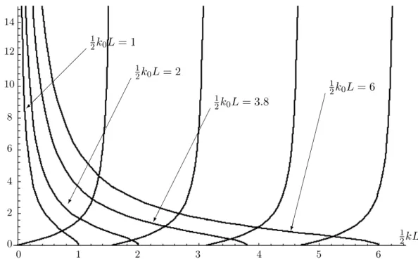
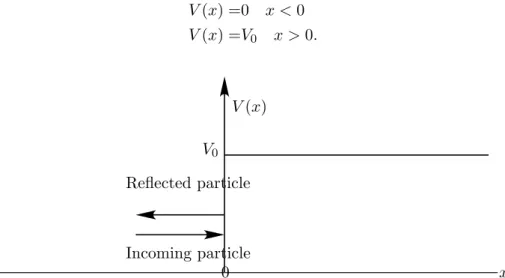
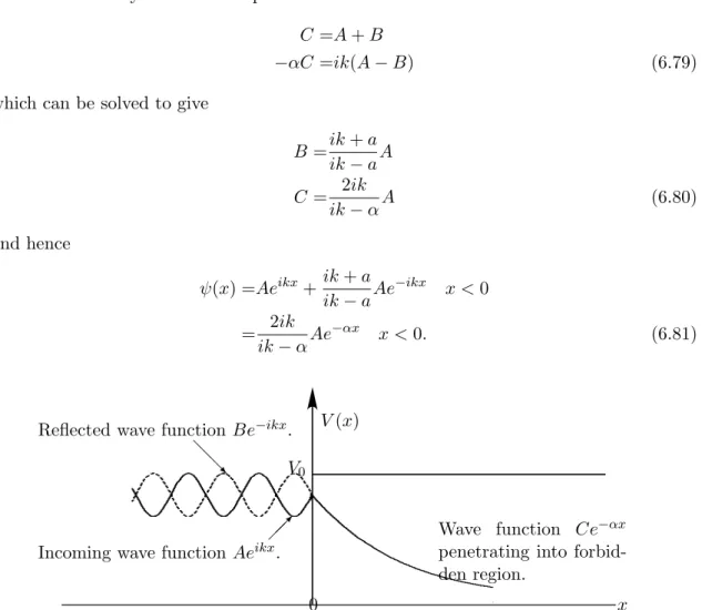
6.1 Derivation of the Schr¨ odinger Wave Equation

We also quote [16] in which the author investigates numerically this relaxed first problem (not only in dimension one), using shape and topological derivatives of the functional

Practical approaches consist either of solving the above kind of problem with a finite number of possible initial data, or of recasting the optimal sensor location problem for

of the Laplacian; indeed we prove that the solutions of the Maxwell- Lorentz equations converge - after an infinite mass renormalization which is necessary in order

cannot work in the general case due to the inexistence of a nice parametrix for hyperbolic equations near the boundary.. The parametrix approach is,

A similar result holds for the critical radial Yang-Mills equation (exponential concentration rate); the same would be the case for (WM) with k = 2. In any dimension N > 6 we

Rendiconti del Seminario Matematico della Università di Padova, tome 42 (1969),

Therefore, we learn from this that the appropriate balance is to offer collaborative learning as a support at the beginning of the course and then reduce it towards the end, as

10 In both experiments the interference pattern from a double slit illuminated by a strongly attenuated red laser was recorded on a photon by photon basis.. The attenuation was