Beyond DCF Analysis in Real Estate Financial Modeling: Probabilistic Evaluation of Real Estate Ventures by Keith Chin‐Kee Leung Bachelor of Commerce, Sauder School of Business University of British Columbia, 2007 Submitted to the Program in Real Estate Development in Conjunction with the Center for Real Estate in Partial Fulfillment of the Requirements for the Degree of Master of Science in Real Estate Development at the MASSACHUSETTS INSTITUTE OF TECHNOLOGY February 2014 © 2014 Massachusetts Institute of Technology. All rights reserved. Signature of Author__________________________________________________________________________________ MIT Center for Real Estate January 30, 2014 Certified by___________________________________________________________________________________________ Richard de Neufville, PhD Professor of Engineering Systems and of Civil and Environmental Engineering Thesis Co‐Supervisor Certified by___________________________________________________________________________________________ David Geltner, PhD Professor of Real Estate Finance and of Engineering Systems Director of Research, Center for Real Estate Thesis Co‐Supervisor Accepted by___________________________________________________________________________________________ David Geltner, PhD Chairman, Interdepartmental Degree Program in Real Estate Development
Beyond DCF Analysis in Real Estate Financial Modeling: Probabilistic Evaluation of Real Estate Ventures by Keith Chin‐Kee Leung Submitted to the Program in Real Estate Development in Conjunction with the Center for Real Estate on January 30, 2014 in Partial Fulfillment of the Requirements for the Degree of Master of Science in Real Estate Development ABSTRACT This thesis introduces probabilistic valuation techniques and encourages their usage in the real estate industry. Including uncertainty and real options into real estate financial models is worthwhile, especially when there is an elevated level of unpredictability surrounding the investment decision. Incorporating uncertainty into real estate pro formas not only provides different results over deterministic models, it changes the angle of attack to real estate valuation problems. When uncertainty is taken into account, the focus shifts from simply maximizing financial returns, to modeling and managing uncertainty to make better ex ante finance and design decisions. The ability to add optionality in probabilistic financial modeling can enhance returns by curtailing losses during downturns and taking advantage of upside conditions. A step‐by‐step example is carefully crafted to demonstrate the simplicity with which uncertainty, Monte Carlo Simulations and Real Options may be included into real estate pro formas. The example is entirely Excel based and is separated into three parts with each progressively increasing in complexity. SimpleCo Tower establishes the familiar Discounted Cash Flow pro forma as a starting point. ModerateCo Tower describes how uncertainty and Monte Carlo simulations can be incorporated into a pro forma while illustrating the effect of non‐linearity on financial models. ChallengeCo Tower reveals how real options can add value to an investment and how it should not be overlooked. The case study illustrates how the techniques outlined in this thesis can add significant value to real estate decisions without much added effort or investment in expensive software. The case study also shows how the use of real world data to model uncertainty can be put into practice. Thesis Co‐Supervisor: Richard de Neufville, PhD Title: Professor of Engineering Systems and Civil and of Environmental Engineering Thesis Co‐Supervisor: David Geltner, PhD Title: Professor of Real Estate Finance and of Engineering Systems Director of Research, Center for Real Estate
Table of Contents
ABSTRACT ... 2 Table of Contents ... 3 Table of Figures ... 5 Acknowledgements ... 6 CHAPTER 1: Introduction ... 7 1.1 Thesis Purpose ... 7 1.2 Format of Presentation ... 8 1.3 Current Industry Practice: Excel, Argus and Discounted Cash Flow Analysis ... 9 1.4 Reluctance to Adopt New Techniques and Reliance on Intuition ... 10 1.5 The Role of Modern Pedagogy in this Thesis ... 12 CHAPTER 2: SimpleCo Tower – A Deterministic Example ... 14 2.1 Assumptions of a Deterministic Model ... 14 2.2 Projecting Cash Flows for SimpleCo Tower ... 14 2.3 Return Measures: NPV and IRR ... 15 CHAPTER 3: ModerateCo Tower ‐ Incorporating Uncertainty into a Financial Model ... 16 3.1 Uncertainty in the Rent Growth Rate of ModerateCo Tower ... 16 3.2 Monte Carlo Simulations and Expected NPV ... 17 3.3 The Flaw of Averages and Jensen’s Inequality ... 18 3.4 A Different Approach to Real Estate Financial Analysis: Distributions and Risk Profiles ... 20 3.5 Static Input Variables versus Random Walks ... 22 CHAPTER 4: ChallengeCo Tower ‐ Managing Uncertainty in Real Estate Projects ... 24 4.1 Real Option Analysis in ChallengeCo using IF Statements ... 24 4.2 ChallengeCo Tower’s Result with a Real Option ... 25 CHAPTER 5: Quantifying Uncertainty in the Real World ... 28 5.1 Predictability in the Real Estate Market ... 28 5.2 Real Estate Economics and the Stock Flow Model for Office Properties ... 30 5.3 Sources of Uncertainty in Real Estate ... 31 CHAPTER 6: Managing Uncertainty in the Real World ... 37 6.1 The Basics of Financial Options ... 37 6.2 Sources of Value for Financial Options ... 38 6.3 The Valuation of Financial Options ... 406.4 Real Options ... 41 CHAPTER 7: Two World Trade Center Case Study ... 44 7.1 Scenario Background ... 44 7.3 Projecting Rents, Cap Rates, Construction Costs and Operating Expenses ... 46 7.4 Pro Formas ... 51 7.5 Real Option Triggers ... 52 7.6 Results ... 53 CHAPTER 8: Conclusion ... 55 BIBLIOGRAPHY ... 57 Appendix A Incorporating Uncertainty into a Financial Model ... 60 Appendix B Performing Monte Carlo Simulations ... 62 Appendix C Creating Cumulative Distribution Functions (CDFs) in Excel ... 64 Appendix D Using IF Statements to Model Real Options for Real Estate Ventures ... 66
Table of Figures
Figure 1: SimpleCo Tower Sketch ... 14 Figure 2: SimpleCo Tower Assumptions ... 14 Figure 3: SimpleCo Tower Pro Forma ... 15 Figure 4: ModerateCo Tower Sketch ... 16 Figure 5: Normal Distribution Curve Used to Model Rent Growth ... 17 Figure 6: Results from the Monte Carlo Simulation ENPV versus Deterministic NPV ... 18 Figure 7: Non‐linearity in the Rent Growth Rate ... 20 Figure 8: ModerateCo Tower Cumulative Distribution Function ... 21 Figure 9: Random Walk Illustration ... 23 Figure 10: Comparison of Returns between ModerateCo and SimpleCo ... 23 Figure 11: Three ChallengeCo Tower Options ... 25 Figure 12: ChallengeCo Tower Expected NPVs ... 26 Figure 13: World Trade Center Site Plan (PANYNJ, 2013) ... 44 Figure 14: 2WTC Rendering (PANYNNJ, 2013) ... 45 Figure 15: Real Estate Cycle Length ... 49 Figure 16: The Regular Sine Curve... 49 Figure 17: 2 WTC Sketch up of Alternatives ... 51 Figure 18: 2 WTC Financial Model Results ... 53 Figure 19: 2 WTC Distribution Function ... 54Acknowledgements
Praises and thanks to God for the blessings throughout my time at MIT. My motivation and drive comes from a sense of purpose that God provides me with. I would like to thank the MIT‐SUTD International Design Center for funding this research. It is my great hope that this thesis could, even in the tiniest way, help empower people to undertake the impossible and design the unexpected. I extend sincere appreciation to Professor Geltner and Professor de Neufville for their wisdom and patience in developing this thesis. I am grateful and honored to have worked with, not only two renowned intellectuals, but two great teachers. I’ll miss the laughs during our weekly meetings in Dr. Geltner’s office. Thanks also to Professor Somerville at UBC for giving me my first break in real estate ‐‐ I’ll never forget it. The MIT CRE faculty and alumni are the best. Thank you for your inspiration. I look forward to our next beer and insightful conversation about real estate and politics. Thanks to the CRE class of 2013 for helping me in the trenches at MIT. It was a battle, but we all made it, together. I can’t imagine life without the RECIII. I am appreciative of my friends who always lift me up when I’m down, especially those at CoL, APG, GCF, BSF, and VCBC. Thanks to AK who makes my day, every day. Thank you to all of my superb former work colleagues for molding my professional character and still providing encouragement even after my departure years ago. Last but not least, a special acknowledgement goes to my family who support me no matter what. We aren’t always a perfect bunch, but when it counts, we are there for each other. Thanks again to all of you. My success is yours as much as it is mine.CHAPTER 1: Introduction “May the odds be ever in your favor.” ‐ Suzanne Collins, author of The Hunger Games In the blockbuster science fiction novel and movie series, The Hunger Games, Collins describes a dystopian society in which a handful of teenagers are engaged in an ultra‐ competitive battle to the death. This competitive environment could draw comparisons to the arena of real estate investing, where deals are won or lost by razor‐thin margins. While Collins’ quote suggests that nothing can be done about one’s odds in the world of her book, this is not the case with real estate. With knowledge of probabilistic valuation methods, real options, and economics, real estate professionals can effectively improve the odds in their favor. 1.1 Thesis Purpose The world of corporate finance was introduced to Monte Carlo methods approximately 50 years ago, significantly altering the valuation approach for derivatives. In contrast, there has not been wide‐spread adoption of stochastic valuation techniques in real estate finance despite the positive track record of Monte Carlo Simulations in corporate finance (Marshall & Kennedy, 1992). The benefits of probabilistic valuation techniques for real estate have been widely documented since the early 1990’s (Baroni, Barthélémy, & Mokrane, 2006; Farragher & Savage, 2008; Louargand, 1992). Yet, the real estate industry still relies on sensitivity analyses for their risk assessment of real estate investments. Farragher and Savage’s 2005 survey of 32 intuitional investors and 156 developers showed that only 2% of these firms utilize Monte Carlo Simulation techniques. The message from academia is not getting through to industry. The rejection of probabilistic techniques by real estate professionals is due, in large part, to the inability of academics to present a compelling argument for probabilistic financial modeling. Academic Key Terms: Stochastic vs Deterministic A stochastic or probabilistic model relies on probability to obtain its values for future states of the system. A deterministic model has no randomness involved in generating its future output values.
theses tend to be excellent at defining what concepts are, but have difficulty with coaching the application of theoretical concepts to the real world. The fragmentation of the research, which occurs because of the multi‐disciplinary nature of the subject matter, inhibits acceptance of stochastic techniques because the true benefits are not realized together in a sweeping overall view from the start of the process, all the way to the end. With roots in engineering, mathematics, economics and finance, the concepts presented in this thesis have never been presented together before. This thesis advocates for the use of probabilistically‐based valuation in the real estate industry by: organizing research from multiple disciplines, demonstrating the great numerical and strategic advantages of stochastic modeling, clarifying how little additional effort is required to achieve those advantages, and emphasizing the applicability of concepts described above to real world problems. This thesis attempts to mend the disconnect between academia and industry by focusing on the effective presentation of ideas and application of modern pedagogical theory. 1.2 Format of Presentation This thesis is structured to appeal to a wide range of real estate professionals. The major, big picture arguments for implementing probabilistic strategies may be of greater importance to executives and managers, while an analyst may want to understand the finer points of modeling uncertainty and real options in Excel. The chapters in this thesis vary in their level of detail. Chapters 2, 3, and 4 walk through a simplified example that incorporates elements of probabilistic valuation at a broad level to demonstrate the main points of this thesis. Discussion in these chapters will tend to be more qualitative. For those looking for a greater detail, the appendix describes how the ideas presented can be implemented into Excel, step by step. Additionally, an Excel workbook of every example is available for real estate practitioners to explore every cell. Chapters 5 and 6 show how the probabilistic concepts translate to the real world, with a detailed case study of 2 World Trade Center to bookend the thesis in chapter 7.
1.3 Current Industry Practice: Excel, Argus and Discounted Cash Flow Analysis The tools of the trade for analyzing income producing properties are Microsoft Excel and Argus. Over the last decade, the ability to work with Excel has become essential in the business world, especially for graduates of business schools. Despite the prevalent usage of Excel in the workplace, generally very few features of the program are used by professionals. Excel users are largely unaware of the computing power available to them and resort to using a handful of common finance calculator functions. However, this is not the fault of professionals, as the user experience, beyond basic calculator functions, becomes unintuitive and frustrating to those not familiar with computer programming. Good coaching and constant practice is required to develop skills beyond basic calculator functions in Excel and this thesis addresses this by providing easy‐to‐follow examples. Argus is software designed to save real estate professionals time by allowing the input of information through a graphical user interface (GUI). A pro forma is generated by Argus once all the information is imputed. Argus, in particular, is useful for organizing lease information and producing rent rolls, a task that is tedious when the analysis is performed manually in Excel. Argus allows real estate analysts to assess the financial feasibility of a deal quicker, enabling a firm to inspect a greater volume of deals. Unfortunately, Argus does have a few drawbacks. While the pro forma is exportable to Excel, Argus does not export the formulas which it uses to calculate its numbers, essentially making Argus a “black box”; the inner workings and logic of the program cannot be inspected. Reliance on the automation which Argus provides to real estate analysts could erode human performance, as practice from working with the nuts and bolts of a real estate pro forma is reduced. A similar argument is made over automation in aircraft cockpits, as reports, such as Sarter & Woods (1994), express concerns over the ability of pilots to react to non‐ normal situations. Another issue is the inflexibility of Argus to adapt to a wide range of real estate ventures. Argus is great at modeling “cookie‐cutter” projects, but its effectiveness is reduced when it’s used to model complex real estate projects. The main method of valuation for income producing real estate is the Discounted Cash Flow (DCF) approach. While the direct capitalization method (using cap rates) is also
widely used, the absolute reliance on one year’s net operating income relegates the direct capitalization method to quick back‐of‐the‐napkin analyses. The DCF approach involves projecting future years of cash flow and discounting them using a risk‐adjusted discount rate to arrive at the Net Present Value of the project. DCF pro formas are taught in introductory real estate and corporate finance courses in universities around the world. There are slight variations in the way the DCF approach is taught from school to school; this does little to deter the widespread usage of DCF pro formas. The deterministic DCF approach does possess limitations, however. First, the analysis of uncertainty is very limited in DCF models. The discount rate reflects the level of risk in a project, but this method oversimplifies risk by relying on single discount rate when there are multiple sources of uncertainty. Also, the discount rate doesn’t take into account the asymmetry between upside and downside risk – generally, downside events matter more to investors than upside events. Thirdly, it ignores the effect of options or possible changes which may occur to the real estate over the life of the investment as owners and managers have flexibility to respond to changes in the economy by making decisions that affect future cash flows. Despite its pitfalls, the DCF approach is well understood at all levels of experience in the real estate industry which makes it a good starting point to discuss probabilistic valuation techniques from. The basic DCF pro forma is highlighted in Chapter 2. 1.4 Reluctance to Adopt New Techniques and Reliance on Intuition Why has the adoption of probabilistic valuation techniques, such as Monte Carlo Simulations, not occurred in the real estate industry? Byrne (1996) suggests that both the small teams and the entrepreneurial nature of the real estate industry prevents the full acceptance of probabilistic methods in financial modeling. But shouldn’t the entrepreneurial spirit of the industry translate into an insatiable appetite to find an edge to get ahead of the competition? Without a doubt real estate teams are small. Whether the teams are based in the largest investment banks or in the largest multi‐national developers, only a few analysts and even
fewer managers are involved in the decision‐making process in any given real estate investment. The heavy workload on open deals could crowd out time available to spend on improving processes, thus perpetuating the status quo. The notion that real estate firms are not embracing stochastic valuation techniques because they are small should be rejected. Real estate firms focus on efficiency and are likely to adopt new methods, processes, or technology if the cost‐benefit rationale makes sense to them. Incorporating uncertainty into the financial analysis of real estate ventures is a “low hanging fruit” and represents a major improvement in analytics with very little effort or cost. Real estate has always been perceived as less sophisticated compared to other asset classes such as stocks or bonds. This perception was largely due to private nature of real estate transactions and the lack of data available for economic analysis. While the market for stocks has been developing since the 1600’s, real estate equity as a securitized asset only began trading in the 1960’s. Without reliable data to guide finance decisions, real estate professionals depended on their instincts and intuition to remain solvent during recessions. As any experienced professional knows, our instincts do fail us from time to time. Part of the reason why uncertainty is overlooked is because it involves seeing financial losses as a possibility. Negativity bias is a psychological phenomenon that may explain what happens when we see losses or experience negative moments (Baumeister, Bratslavsky, Finkenauer, & Vohs, 2001). A common example of this effect is the anti‐anticipation and stress of receiving a large restaurant bill, which is further exacerbated if the actual bill amount is unknown. Humans tend try to avoid these negative experiences that shake our confidence even if great benefits are possible. Previously published research advocating for the use of probabilistic valuation techniques were missing a key component: data from a sufficient number of market cycles to describe the behavior of market factors and uncertainty. With over 50 years of data available, the time is ripe for real estate to explore scientific approaches. Appropriate usage of real estate data from indices are discussed further in chapters 5 and 6.
The techniques described in this thesis will not eliminate the need for good instincts in real estate, but rather, they will enhance decision‐making by providing different perspectives on real estate problems. 1.5 The Role of Modern Pedagogy in this Thesis The struggle of university researchers to connect with learners is well documented (Seymour, 2008). The academic tenure system is cited as a major reason why teaching and communication have taken a back seat, as professors are encouraged to push out publications more than developing teaching skills. If professors have difficulty keeping students in their classrooms engaged, what hope do they have in trying to engage readers in a one‐way medium? Indeed, scholarly articles seem to be more effective in communicating ideas to other academics, but what about the rest of society? The main intent of this thesis is present probabilistic concepts to real estate professionals with a high level of clarity. Often times, authors of scholarly articles enter into auto‐pilot mode and deliver their ideas based on their own experience as learners or casual observations. For this thesis, special attention is paid to pedagogy to prevent a researcher‐ centered teaching approach and move towards a learner‐centered approach. As you might imagine, there is no scarcity of research on how adults learn. Described below are two major theories in modern pedagogy which guide the manner of presentation for concepts introduced in this thesis. The first theory is of mental models, or schemas. Child psychologist Jean Piaget proposed a process in which children use their interactions with the world to develop models of objects and patterns of action (Lang, 2008). It turns out that what we know already about the world greatly influences how we encounter new experiences; our existing models are under constant revision. When adults are met with new experiences or ideas, they work to fit these new elements in to patterns which they already understand. There are two learning processes which can occur when a person encounters a new experience: assimilation and accommodation. Assimilation occurs when a person takes in a new idea by making the idea fit to into their existing models. On the other hand, accommodation occurs when the new idea does not fit into any pre‐existing models and changes are made to a person’s existing models to take in the new information.
Awareness of both these processes is crucial to effective delivery of the ideas presented in this thesis. In some scenarios, assimilation needs to occur which requires the presenter to help the audience connect to pre‐existing knowledge. An example of this occurring in this thesis is the use of the familiar Discounted Cash Flow pro forma as a starting point for more complex feature additions. For scenarios in which accommodation is likely to occur, clarity is vital to cease the perpetuation of common misconceptions and pitfalls. Clarity is emphasized when presenting the Flaw of Averages in Chapter 3. Bloom’s Taxonomy is the second pedagogical theory that is applied in this thesis. Bloom’s Taxonomy is a framework developed by Benjamin Bloom in 1956 to categorize learning objectives. The framework divides educational objectives into three domains: cognitive, affective, and psychomotor (Krathwohl, 2002). Skills in the cognitive domain include those of knowledge and critical thinking. The affective domain include skills relating to emotion, while the psychomotor domain focuses on skills with physical tools, such as hammers. The cognitive domain is most relevant for the concepts presented in this thesis. In the revised Bloom’s Taxonomy, Krathwohl presents 6 levels of processes in the cognitive domain. From lowest complexity to highest, they are: remember, understand, apply, analyze, evaluate and create. If the goal is to teach professionals how to create their own simulations, the corresponding discussions and examples should match that goal in detail and complexity. Since chapters in this thesis vary in their objectives (some professionals might only want to go up to ‘understand’ level, while other will want to ‘create’), careful attention is paid to maintain consistency in cognitive levels. Mismatched objectives and discussions lead to frustration for readers. The appendices and chapters 5, 6, and 7 cater to readers who want to reach the ‘create’ level, while next 3 chapters reside at the ‘understand’ level. We begin gently by walking through the deterministic discounted cash flow pro forma.
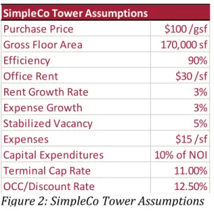
CHAPTER 2: SimpleCo Tower – A Deterministic Example The first example, SimpleCo Tower, is a simplified discounted cash flow pro forma of the kind analysts typically use to financially model commercial real estate transactions. SimpleCo Tower is a 10 story office tower with a floor plate of 17,000 sf. A financial model is created to evaluate the purchase of the building for a price of $17 million. There are three major sections to a pro forma: the assumptions, the cash flow projections, and the outputs. 2.1 Assumptions of a Deterministic Model The assumptions are a set of parameters with which the financial model most abide by. Some assumptions are physical (such as floor area and efficiency), while others are economic (such as rent and discount rate.) Estimating the assumptions accurately is important because they drive all numbers in the pro forma. 2.2 Projecting Cash Flows for SimpleCo Tower The cash flow projection section of the pro forma projects many line item several years into the future. Variables in the formulas are often linked or referenced to the assumptions on this page. The cash flow projection organizes the revenues and costs associated with a particular property and calculates the net cash inflows/outflows for each year of property ownership. In SimpleCo Tower, the Property before Tax Cash Flow (PBTCF) is calculated without the effects of income tax or leverage. Figure 1: SimpleCo Tower Sketch A visual representation of the 10‐ story office tower, SimpleCo Tower. Purchase Price $100 /gsf Gross Floor Area 170,000 sf Efficiency 90% Office Rent $30 /sf Rent Growth Rate 3% Expense Growth 3% Stabilized Vacancy 5% Expenses $15 /sf Capital Expenditures 10% of NOI Terminal Cap Rate 11.00% OCC/Discount Rate 12.50% SimpleCo Tower Assumptions Figure 2: SimpleCo Tower Assumptions This chart can be viewed in the SimpleCo Excel file on the CD.
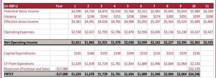
2.3 Return Measures: NPV and IRR The output section of a DCF pro forma calculates the objective return measures. In the world of finance, no return measure is as prevalent as Net Present Value (NPV), or its sibling the Internal Rate of Return (IRR). For SimpleCo Tower, our NPV at a 12.5% discount rate is ‐$135,000 and the IRR is 12.37%. SimpleCo Tower is a deterministic model. For each unique set of assumptions there is one sole outcome. The output (NPV in this case) is determined by the input assumptions to the exact cent. There is no uncertainty in the model because a set of assumptions always lead to a sole output return measure. Pressing the “F9” key recalculates formulas in Excel, but doing so will never change the NPV in the SimpleCo Tower pro forma. (in 000's) Year 1 2 3 4 5 6 7 8 9 10 11 Potential Gross Income $4,590 $4,728 $4,870 $5,016 $5,166 $5,321 $5,481 $5,645 $5,814 $5,989 $6,169 Vacancy $230 $236 $243 $251 $258 $266 $274 $282 $291 $299 $308 Effective Gross Income $4,361 $4,491 $4,626 $4,765 $4,908 $5,055 $5,207 $5,363 $5,524 $5,689 $5,860 Operating Expenses $2,550 $2,627 $2,705 $2,786 $2,870 $2,956 $3,045 $3,136 $3,230 $3,327 $3,427 Net Operating Income $1,811 $1,865 $1,921 $1,978 $2,038 $2,099 $2,162 $2,227 $2,293 $2,362 $2,433 Capital Expenditures $181 $186 $192 $198 $204 $210 $216 $223 $229 $236 CF From Operations $1,629 $1,678 $1,729 $1,781 $1,834 $1,889 $1,946 $2,004 $2,064 $2,126 Reversion (Purchase and Sale) ‐$17,000 $22,120 PBTCF ‐$17,000 $1,629 $1,678 $1,729 $1,781 $1,834 $1,889 $1,946 $2,004 $2,064 $24,246 Figure 3: SimpleCo Tower Pro Forma The cash flow projections are shown for SimpleCo Tower. This chart can be viewed in the SimpleCo Excel file on the CD. Net Present Value and IRR The time value of money principle is the most fundamental in finance. Cash flow today is worth more than cash flow in the future because of interest earning potential. Future cash flows are discounted to arrive at an equivalent value today called the Present Value (PV). Net Present Value is the sum of the PVs of all future cash inflows and outflows of a project. The Internal Rate of Return (IRR) is the discount rate which makes NPV equal 0.
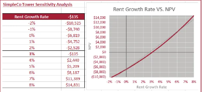
The NPV can change if an assumption is manually altered. The effect on NPV of a change in an assumption can be recorded in a sensitivity analysis. Utilizing a data table in Excel, the change in NPV can be seen when one or two variables change (a sensitivity analysis is performed on the rent growth rate in section 3.3). Unfortunately, this analysis is limited to two variables and the real world usually doesn’t “hold all else constant”. What alternatives are out there for financial modeling? CHAPTER 3: ModerateCo Tower ‐ Incorporating Uncertainty into a Financial Model Most real estate professionals are familiar with the techniques described in the SimpleCo Tower pro forma because the deterministic DCF model is taught in many introductory finance courses around the world. ModerateCo Tower expands on the SimpleCo Tower pro forma by adding uncertainty to one of the assumptions, the rent growth rate. Everything else about ModerateCo is the same as SimpleCo. 3.1 Uncertainty in the Rent Growth Rate of ModerateCo Tower The SimpleCo Tower example assumed that the rent growth rate was 3% per year. Based on the averaging of historic rent growth rates, 3% is a common assumption among real estate professionals. When the rent growth rate is subject to uncertainty, it is acknowledged that the true rent growth rate is unknown and varies within a range. Excel’s random number function is used to simulate uncertain behavior. Appendix A goes through step‐by‐step how uncertainty was built in to the ModerateCo Tower financial model. Figure 4: ModerateCo Tower Sketch A visual representation of ModerateCo Tower, a 10‐story office tower that is physically identical to SimpleCo Tower.
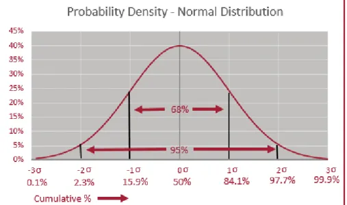
In ModerateCo, the uncertainty is created as a symmetrical Normal distribution around a mean. Using 3% as the mean for the rent growth rate, there should be an equal chance for the growth rate to appear above or below 3%. 3.2 Monte Carlo Simulations and Expected NPV Once the financial model has input assumptions that randomly change, the corresponding output NPVs can be recorded many times using a Data Table in Excel. The process of running a model for a specified number of iterations is simply called a Monte Carlo Simulation. The NPV will vary from simulation to simulation because the input variables are always changing. In the case of ModerateCo, the input variable, Rent Growth Rate, changes. Also known as a ‘Gaussian Distribution’, a random variable is ‘normalized’ according to this distribution. The RAND function in Excel fetches a random number between 0 and 1 and is centralized towards the mean. For example, if the number comes out to be .159, it will be placed ‐1 standard deviation from the mean. 68% of values (.159 to .841) will fall within 1 standard deviation of the mean. Figure 5: Normal Distribution Curve Used to Model Rent Growth Monte Carlo: What’s in a name? As a favorite hangout of Ian Fleming’s fictional character James Bond, Monte Carlo is often associated with luxurious, mysterious and exotic living. Perhaps, Monte Carlo Simulations sound more foreign then they actually are. “Monte Carlo” Simulation just refers to a simulation where the number of iterations are set by the user. For example, we run 5,000 iterations for ModerateCo Tower, not one more nor one less.
The input variable could be 2% leading to a certain NPV value, and in the next iteration, the rent growth rate could be 3.5%, leading to a higher NPV value. After running 5,000 iterations of the model, ModerateCo Tower calculates the mean of the 5,000 NPVs to yield an Expected Net Present Value (ENPV). In this case, the mean of the simulated NPV (ModerateCo) will be consistently greater than the deterministic NPV (SimpleCo) even though 3% was used as the mean in ModerateCo. In other words, even if multiple sets of 5,000 simulations were ran, the simulated ENPV of ModerateCo will generally be significantly greater than the NPV of SimpleCo. How could this difference occur? Shouldn’t the SimpleCo NPV and ModerateCo ENPV be the same if we ran many simulations of ModerateCo? Intuition may try to apply the Central Limit Theorem or Law of Large Numbers in this case. As the number of iterations of a random independent variable becomes very large, the variables will be normally distributed around the expected value (if using the NORM.INV function). In fact, there should be close to an equal number of occurrences of rent growth rate above and below the mean rent growth rate in ModerateCo since we are using a symmetrical normal distribution to model the uncertainty in the rent growth rate. While the input variable behaves this way with the expected value as its mean, this actually does not extend to the output NPV. The Flaw of Averages explains why. 3.3 The Flaw of Averages and Jensen’s Inequality First coined by Savage, Danziger, & Markowitz (2009), the Flaw of Averages is a major error that occurs when using averages in deterministic models instead of proper stochastic variables. De Neufville & Scholtes (2011) describe the Flaw of Averages as the widespread‐ Figure 6: Results from the Monte Carlo Simulation ENPV versus Deterministic NPV Interesting result! The simulated ENPV is an expected NPV because it is just an average of all the results in a Monte Carlo Simulation. In this case, ModerateCo’s NPV was recorded 5,000 times and averaged to get an average of $375,575. The deterministic NPV is taken directly from the SimpleCo pro forma. This result can be viewed in the ModerateCo Excel file.
but‐mistaken assumption that evaluating a project around average conditions give a correct result. The simple math behind the Flaw of Averages concept is based on Jensen’s Inequality. In 1906, Danish mathematician Johan Jensen proved that: Basically what happens is a symmetrically distributed input variable leads to an asymmetric distribution of output values. When this occurs, the system or model is described as non‐linear. The SimpleCo model is a perfect example because it’s pro forma uses a 3% historic average for its rent growth. When the deterministic 3% is replaced with an input random variable symmetrical distributed around 3%, the output NPV value ends up significantly greater for ModerateCo over SimpleCo! The source of non‐linearity in this case is annual compounding. The same effect that makes compound interest (non‐linear) greater than simple interest (linear) at the same rate generates the difference in returns between SimpleCo and ModerateCo. For ModerateCo Tower, 3% is the mean growth rate, so a 2% growth rate and a 4% growth rate should occur with equal probability. Because the curve is convex (due to compounding), going up to 4% results in a greater upward NPV improvement [|2440‐(‐ 135)|= 2,575] than the NPV erosion of going down to a 2% growth rate [|‐2,528‐(‐135)| =2,393]. Systems behave asymmetrically when upside and downside effects are not equal. Jensen’s Inequality The average of all the possible outcomes associated with uncertain parameters is generally not equal to the value obtained from using the average value of the parameters.
The Flaw of Average has a significant impact on NPV and could spell the difference between winning a bid and losing a bid, as exemplified by the SimpleCo and ModerateCo comparison. 3.4 A Different Approach to Real Estate Financial Analysis: Distributions and Risk Profiles Incorporating uncertainty into real estate pro formas not only gives a different result over deterministic models (as per the Flaw of Averages), it changes the approach to real estate valuation problems. In the deterministic SimpleCo Tower case, the strategy is to lock in a set of ex ante assumptions based on the analyst’s best forecast, find the single best value and hope for the best. When uncertainty is factored in to the analysis, the focus shifts to modeling and managing the uncertainty to make better finance and design decisions today. The single best expected value of NPV is no longer the sole objective in a stochastic model: range and distribution of outcomes become relevant. Let’s say that we have two iterations of the model. In one iteration, the rent growth rate is 2%, and the other is 4%. Leading to a NPV result set of ‐2,528 and 2,440. If we average these two values, we get ‐44 which is higher than the result we would get at 3% of ‐$135! The difference becomes greater and greater as values further from the mean are used. This sensitivity analysis of the rent growth rate can be found under the SimpleCo pro forma, in the SimpleCo Excel file. Figure 7: Non‐linearity in the Rent Growth Rate
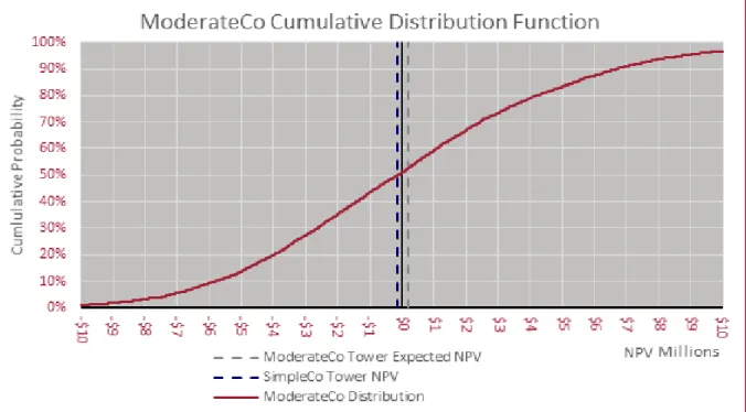
Introducing a realistic level of randomness into financial models changes the framing of the valuation problem. Understanding the likelihood of losing or profiting become important once we introduce uncertainty into the analysis. The cumulative distribution function (CDF) of ModerateCo provides information on the probability of loss or profit scenarios. ModerateCo has about a 50% probability of having negative NPV and a 50% probability of a having a positive NPV. The downside probability is more limited than the upside probability, as illustrated by the long tail towards the right (more positive NPVs). This scenario is a typical observation for real estate projects. Ideally, an analyst will want to manage the uncertainty by finding ways to limit the downside losses and accentuate the upside profits. Other useful measures that come out of this analysis of distributions include Value at Risk and Value at Gain. Value at Risk denotes how much loss could occur at a specified probability over a time frame. In the ModerateCo example, the Value at Risk (V10 number) On the CDF, the likelihood of NPV outcomes is displayed as well as the NPV for the deterministic SimpleCo Tower and the probabilistic expected NPV for ModerateCo Tower. This chart and its corresponding Monte Carlo Simulation is included in the ModerateCo Excel file, on the ‘ModerateCo Distribution” tab. Figure 8: ModerateCo Tower Cumulative Distribution Function
NPV is ‐$6 million. That is, there is a 10% probability that a negative $6 million NPV or worse will be incurred over the 10 year life horizon of the investment. On the other side, the “V90 NPV” is $7 million. This Value at Gain “V90” number can be read as: There is a 10% chance that the NPV for the project over the 10 year investment horizon will be over $7 million. 3.5 Static Input Variables versus Random Walks The rent growth rate’s behavior in the ModerateCo model is currently a static variable. Once a rent growth rate is randomly generated for a scenario, it remains the same for the life of the investment. Deterministic pro formas frequently model input assumptions as a static variable because the basis for their assumptions are from historic averages of long‐ term annual rates. Economic conditions change over the life of a long‐lived investment and deterministic financial models are poor at modeling this behavior. Since ModerateCo’s input variables are randomly generated and do not rely on historic averages, a change over time over can be modeled in to the annual rent growth rate. Growth rates generally do not move independently from year‐to‐year with absolute randomness; rates tend to vary around the results from the preceding period. Pearson (1905) described this behavior as a “Random Walk”. A random walk modeled into a pro forma will allow an investment’s profitability performance to decline and recover over the investment horizon. This up and down behavior is essential to the modeling of real options in the proceeding chapter.
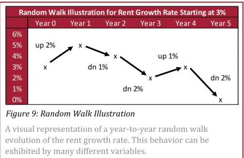
The additional variability translates into greater volatility in the results of the Monte Carlo simulation and amplifies effect of the Flaw of Averages. The strong effect of the Flaw of Averages and Random Walk volatility should be enough motive to start modeling real estate using probabilistic techniques. The thesis continues to make the case for stochastic valuation of real estate in ChallengeCo Tower by using Real Options. A visual representation of a year‐to‐year random walk evolution of the rent growth rate. This behavior can be exhibited by many different variables.
Year 0 Year 1 Year 2 Year 3 Year 4 Year 5 6% 5% up 2% x 4% x 3% x x 2% x dn 2% 1% 0% x dn 1% dn 2% up 1% Random Walk Illustration for Rent Growth Rate Starting at 3% Figure 9: Random Walk Illustration
Results ENPV St. Dev.
ModerateCo $192,043 $4,920,803 ModerateCo w/ Random Walk $1,042,254 $9,240,832 SimpleCo Deterministic NPV ($134,701) Figure 10: Comparison of Returns between ModerateCo and SimpleCo Random‐walk behavior adds greater volatility to the model which inflates the effect of the Flaw of Averages even further. The Monte Carlo Simulations and results can be viewed in the ModerateCo Excel file.
CHAPTER 4: ChallengeCo Tower ‐ Managing Uncertainty in Real Estate Projects With distributions, we gather information that will aid us in finance decision‐making. This chapter focuses on how to use this information advantageously. Real option analysis is utilized to explain the impact of adding flexibility into the design or financial models. A Real Option is described specifically as a “right without an obligation”. Chapter 6 provides a detailed discussion on Real Options, but for now, a basic option to add more floors in the future to the on‐going example of SimpleCo and ModerateCo towers will be described. ChallengeCo does not stray much from the enduring example. The subject building is still a 10 story office building. However, ChallengeCo Tower is now an investment in a 10 story development project instead of a pre‐existing stabilized office tower. Rather than a purchase price, we use a development cost to build the project. An option to build 10 additional floors in the future is examined further in the ChallengeCo Tower pro forma provided in the ChallengeCo Excel file. Almost all input assumptions are subject to uncertainty using the same NORM.INV function described in ModerateCo. Additionally, the input assumptions will exhibit “random walk” behavior, with the preceding year’s value used as the mean for next year’s value. Each input assumptions will go through their own random walks, culminating into a specific NPV for a unique 10 year unique state of the world. 4.1 Real Option Analysis in ChallengeCo using IF Statements Using IF statements in Excel, real options can be modeled with ease. Two pieces of information are required to model real options. Firstly, the “trigger” conditions need to be specified: What conditions need to occur before the option is exercised? Secondly, the exercise costs and other consequences of the option need to be identified: What is the effect if the option is actually exercised? Once these two pieces of information are detailed, the option can be modeled into the pro forma. The objective here is to model the option in such a way that the consequences of an exercised option are automatically displayed in the pro forma if the predetermined conditions occur. Then, a Monte Carlo Simulation examines the
effects of the option on the NPV in comparison with an identical development without the option. Appendix D, discusses the use of “if statements” to model real options in greater detail. For ChallengeCo, three separate pro formas are created to show the difference in expected NPV and distributions. One pro forma calculates the NPV for a development project with a flexible design option built‐in to the model to construct an additional 10 floors at a later date. The second pro forma calculates the NPV for a standard 10 story development with no option built‐in. The third pro forma calculates the NPV for a 20 story development without an option built‐in to the design. 4.2 ChallengeCo Tower’s Result with a Real Option The results from the Monte Carlo Simulations show that design flexibility can have a significant financial value. While the development with flexibility never dominates the two option‐less alternatives (the flexible alternative distribution function is always to the left of either the 10 story or 20 story distribution function), the results show how the flexible alternative can be advantageous. Figure 11: Three ChallengeCo Tower Options The building on the left represents the Inflexible ChallengeCo project at 10 floors. It is physically identical to ModerateCo and SimpleCo Towers. In the middle shows a flexible design where an additional 10 floors can be built on top of the first phase of 10 floors. On the right is the inflexible 20 floor ChallengeCo Tower.
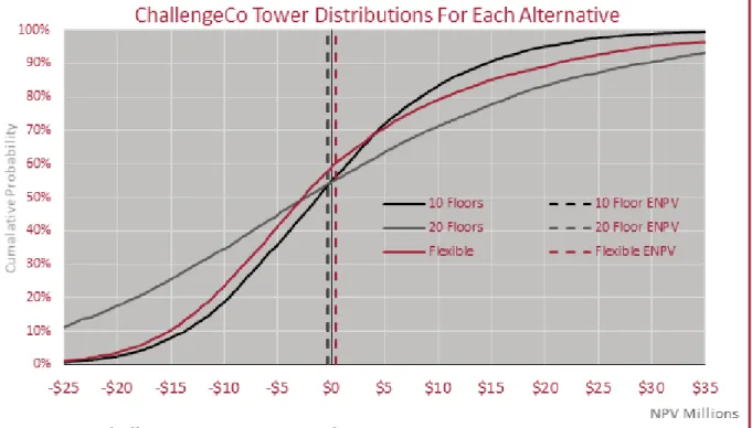
If economic conditions turn sour in the next 10 years, the option to expand is not exercised and the distribution function of the flexible alternative “hugs” the 10 floor inflexible option. In poor economic times, the flexible option will not perform as well as the 10 floor inflexible development because some extra construction costs are “sunk” into the initial construction cost of the flexible alternative (for example, constructing stronger columns to take the load of a possible 10 floor addition). On the other hand, the flexible alternative performs much better than the 20 floor inflexible development during a poor economy. When economic conditions are good, the flexible alternative takes advantage of the upside by exercising its option to build more space. This is illustrated when the 10 floor inflexible alternative is compared with the flexible option above the $5 million NPV mark. The Figure 12: ChallengeCo Tower Expected NPVs The CDF shows how the flexible design (in red) uses the real option to take advantage of upside conditions. At the low end, the flexible design does not exercise its option to expand, so its CDF curve closely follows the curve of the 10 floor inflexible design. If economic conditions are good, the flexible design begins to deviate from the 10 floor inflexible design by exercising its option to expand and follows closer to the 20 floor inflexible design curve to take advantage of the good economy. The Monte Carlo Simulations and CDFs can be found in the ChallengeCo Tower Excel file.
flexible alternative will deviate from the 10 floor inflexible alternative and capitalize on the opportunity of great market conditions. The expected NPV of the flexible alternative is the greatest among the three alternatives for ChallengeCo Tower. For investors seeking to limit their downside exposure, while taking advantage of the upside as much as possible, flexibility can be a major win. Flexibility in design should not be overlooked when making investment decisions.
CHAPTER 5: Quantifying Uncertainty in the Real World The example presented in Chapters 2 to 4 is simplified to underline the importance of including uncertainty and managing the risk that exists in real estate investing. In this chapter, the focus shifts to the execution of these techniques in the real world. To implement stochastic techniques into a real world financial model, the inputs that are subject to uncertainty must be quantified with a decent level of accuracy or the outputs cannot be trusted – the computer science axiom, “Garbage In, Garbage out” is appropriate here. Accuracy is important, but how precise or detailed should a financial model be? The real estate industry has embraced the DCF method which, as demonstrated by the Flaw of Averages in chapter 3, is generally less accurate and much less detailed than the simplest stochastic models. From this casual observation, perhaps professionals put more stock in accuracy (getting close to the actual number) rather than detail. There is a possibility of increasing the complexity of a financial model so much that the major fundamentals of the pro forma are washed out; losing sight of the “forest through the trees”. Thus, it is important that increasing detail is not pursued at the expense of accuracy. The discussion herein is science based, but the implementation of these concepts remains an ‘art’ requiring real estate intuition. 5.1 Predictability in the Real Estate Market In the 1960’s, a powerful theory emerged called the Efficient Market Hypothesis (EMH) with contributions from economists such as Paul Samuelson and Eugene Fama (Malkiel & Fama, 1970; Samuelson, 1965). Their work explains how the stock market is so efficient and quick to adapt to new information that it is impossible to predict where the market is going, since future information is unpredictable. By extension, the stock market should behave as a complete random walk (Fama, 1995). Looking at historic trends is futile because future information occurs independently from what has already happened. Exchange traded funds (ETFs), which are funds which try to replicate the entire market, were created to make use of the EMH mantra, “active management of funds won’t help”. In fact, Fama & French (2010) show that 65% of actively managed high fee mutual funds did not beat passively managed ETFs.
In recent years, the EMH has been challenged by research that argues for a level of predictability existing in the markets. Lo & MacKinlay (1988) used new data to reject the idea of the markets behaving as a random walk. Jegadeesh & Titman (1993) discovered that momentum in the stock market can lead to above market returns; that is, relying on the short term tendency for a stock’s price to go up if it was going up the last period. Shiller (1990) proposed that a mean‐reverting behavior exists in the stock market due to investor irrationality. Alas, some level of predictability exists which can be used advantageously which keep financial analysts like the author of this thesis employed. While weakened from modern empirics and the 2008 financial crisis, the EMH still affects the way investors’ model future returns by cautioning market participants about how difficult it is to earn above‐market returns. In addition, the EMH highlights the important role which uncertainty plays in the market. Do these theories primarily focused on the stock market translate over to real estate? Yes and no. For variables in the office space market such as rent and vacancy, a level of predictability does exist due to patterns in momentum and cyclicality which are discussed in greater detail later in this chapter. In real estate asset markets, the EMH holds less weight compared to stock exchanges, because the cash flows of real estate asset (which are dependent on the space market) are fairly predictable. In general the EMH suffers from a lack of applicability to real estate because of the heterogeneity of real estate, the lack of public sales information, and time lags in the transaction process. On the other hand, Real Estate Investment Trusts (REITS) can behave similarly to the rest of the public capital markets. Generally, the more efficient a market is at integrating new information in asset prices, the less predictable it is. The predictive nature could even become endogenous to the price of an asset in a very efficient market. For example, when a new technique is developed and proven to be capable of making above‐market risk adjusted returns, everybody will immediately copy the technique which becomes the new standard. The main takeaway from this section is that most real estate markets behave with both predictability and randomness at the same time and this should be reflected in the way financial models are created.
5.2 Real Estate Economics and the Stock Flow Model for Office Properties The mechanics of how real estate prices move over time has been studied extensively and can be described using a Stock Flow Model. A Stock Flow model is simply any model which describes the process of how a durable stock of goods, such as real estate, increases and decreases and interacts over time with the flow of usage (i.e. leasing) of that stock of goods. To start off, the Stock Flow Model draws on the familiar concept of supply and demand, with a few quirks, to correctly describe what occurs in real estate. Employment is the driver for rent of office space on the demand side. On the Supply side, the stock of office space is the main determining factor. The stock of office space is completely inelastic in the short‐term because office buildings take time to build, When demand (employment) increases, the rent must increase because it takes time for new stock to arrive in the form of new construction. When employment fall, rents will fall by a greater percentage because of the durability of real estate capital leading to complete inelasticity in supply in the short run. New real estate stock is gradually introduced into the market to meet demand and because of this, rents and prices react quickly to changes in the demand, but stock does not. What triggers new construction? Asset prices – which are a function of rents and cap rates. Di Pasquale & Wheaton (1996) illustrates these relationships between construction, asset markets and space markets in the Four Quadrant model. As the economy goes through its ups and downs, real estate prices and rents go up and down because demand changes without a quick response from the supply side due to the durability of real estate and lag to deliver new space. Eventually, increases in rents and prices promote new construction which gradually alleviates pressure on rents as the new space is delivered to market. Since there is a time lag in construction, it is rare that the exact amount of completions comes online and perfectly meets demand; there will be overbuilding and underbuilding which leads to real estate incurring its own cycle. The variables required to create a stock flow model can be obtained by using linear regression techniques on a large result set of reliable historic data. Multiple linear regression attempts to quantify the relationship between a dependent variable and multiple independent variables. For example, a regression can be ran between the square
footage of occupied space and employment, a major driver of office demand. If the numerical relationship can be predicted, forecasting employment (a source of demand) will lead to a prediction for occupied space. In terms of complexity, uncertainty can be incorporated at different levels in a financial model. Some analysts will prefer to model uncertainty into rents directly, while others will prefer to add uncertainty to more primal sources such as employment growth and run these numbers through a stock flow model to arrive at rents. Please refer to Paradkar's (2013) thesis for a model which incorporates uncertainty using the stock‐flow model. 5.3 Sources of Uncertainty in Real Estate There are infinite possibilities when it comes to events or shocks that may influence real estate asset values and rents. Uncertainty can be driven by changes in the macro‐economy and local economy. Technological innovation such as hydrologic fracking come out of the blue to effect office markets catering to the energy sector. Transportation infrastructure changes give rise to winners and losers in real estate. The endless list of potential shocks need to be simplified into a few sources before they can be quantified! With the help of recent innovations in real estate indices, 7 important forms of uncertainty can be quantified: long‐run market trend, long‐run market cycle, market volatility, short‐ run inertia, individual asset specific volatility, individual asset pricing noise, and ‘Black Swans”. Long‐run Market Trend: This is the straight line appreciation trend which prevails over the long term in the real estate asset market. Research into residential real estate trends have found that over the super‐long term (over the course of a century), prices appreciate close to the rate of inflation (Eichholtz, 1997). Growth in commercial real estate over the long haul has been found to be slightly less than inflation because of depreciation (Fisher, Geltner, & Webb, 1994; Wheaton, Baranski, & Templeton, 2009). With this knowledge, professionals may be tempted to input 1% or 2% because of the stability the Federal Reserve Bank offers for inflation in the United States, but keep in mind that investment horizons for commercial real estate tend to be shorter than 20 years.
Long‐run Market Cycle: The long‐run market cycle is the oscillating nature of real estate prices that is easily observable on a time‐series graph. The peak‐to‐peak or trough‐to‐ trough timing has been between 15 and 20 years in last few commercial real estate cycles. Wheaton (1999) explains how there are two ways in which the real estate market could manifest itself. One view is that real estate developers are completely rational and forward‐ looking while the other view is that developers are backward‐looking (or ‘myopic’) when forecasting future supply and demand. When agents are rational and forward looking, they have a good understanding of how the market behaves with uncertainty, so prices reflect the present value of future cash flows and the uncertainty surrounding the cash flows. A practice which would classify as “myopic” behavior include extrapolating average historic rates forward in financial models. In Wheaton’s simulations, he finds that both cases still (myopic or forward‐looking) generate endogenous long‐run cycles within real estate as developers struggle to forecast the exact amount of space to build. Market Volatility: Zooming in a little bit from the Long‐run Market Cycle level, there is volatility which exists month‐to‐month and year‐to‐year along the cycle preventing a smooth oscillating curve. Events that can influence this type of uncertainty include natural disasters or announcements by central banks. Any new discovery of information that provides a shock that the market takes time to adjust to are uncertainties related to market volatility. Short‐run inertia: Also called momentum, this is the tendency for prices that are rising to want to keep rising – or falling prices to keep falling. To measure inertia, auto‐regressive techniques are employed which measures the level of influence a previous period’s price movement has on the current period’s price change. If the relationship is high between the prices for the two periods, it means that people are using the current period’s price as a basis to forecast future periods. It is interesting to note that inertia is very weak in data involving REITs because of how efficient securities markets are. The frictions in private real estate markets, however, allow momentum to occur. Individual Asset Volatility: If a financial model focuses in on a particular property, the model will be subject to idiosyncratic asset volatility, that is, risk which is specific to an individual
asset that doesn’t apply to the rest of the market. For example, a municipality might announce a new rapid transit station to be constructed next to an office tower which created an unexpected boost in the office property’s value. Individual Asset Pricing Noise: In the private real estate market, every professional will have differing opinions on the value of a property. If polled, the opinions of value for thousands of real estate experts might be scattered around the ‘most likely’ value, with a greater spread for more unique properties and less of a spread for properties with multiple comparables. Noise is the effect that these differing opinions have on the pricing of real estate. Appraisers take into account noise when they provide a range of prices that they believe a specific property can sell for. Black Swans: In defining what Black Swans events are, Taleb(2007) states: “first, it is an outlier, as it lies outside the realm of regular expectations, because nothing in the past can convincingly point to its possibility. Second, it carries an extreme impact. Third, in spite of its outlier status, human nature makes us concoct explanations for its occurrence after the fact, making it explainable and predictable.” Any event with major impact on real estate values encompasses this risk. For example, a new renewable energy source (making combustion engines obsolete) suddenly discovered in a lab at MIT could have major “Black Swan” type ramifications for real estate. Each type of uncertainty described above can be quantified on their own. Then a Monte Carlo Simulation outputs the effect of uncertainty as a whole on a real estate project. Modeling the effect of 7 types of uncertainty together without a Monte Carlo Simulation would be practically impossible. 5.4 Real Estate Indices Real Estate indices provide some of the data from which the 7 forms of uncertainty can be extracted. There are many choices with regards to real estate indices, with each having their own advantages and disadvantages. There are three major types of real estate indices in the United States: appraisal‐based, transactions‐based, and stock market based (Geltner, 2014).
Appraisal‐based indices use independent professional appraisals of properties to track real estate markets. They were the earliest forms of indices in real estate, so they tend to have longer histories. The major drawback with appraisal‐based indices is that they are susceptible to a phenomenon called appraisal smoothing. Appraisers tend to use empirical information such as sales comparable to determine the current value of properties which develops a lag in their estimated value. This lag contributes to a smoothing effect on the index which reduces the apparent systematic risk in the real estate returns. Transactions‐based indices (TBI) use actual sales data of commercial real estate to track the market. To accomplish this, many of these indices monitor pairs of sales on properties to ensure that the changes reported are from an apples‐to‐apples comparison. TBIs are relatively new with data only stretching back to 2000 but they hold great promise because the underlying transaction price data not only quantifies market volatility reflected in the indices themselves, but also quantify individual asset idiosyncratic uncertainty using the residuals of the price regressions. Stock market‐based indices track the movement of publicly traded real estate investment trusts. Because each REIT generally specializes in one property type or another, they can be a great source of data when looking at a particular geographical area or industry. Keep in mind that REIT values do not perform the same as private real estate all the time. The efficiency of the stock market eliminates much of the inertia that would exist in the private market. In addition, there is evidence that the REIT market slightly leads the private real estate market (Barkham & Geltner, 1995). 5.4 Translating Data on Uncertainty into a Pro Forma Quantifying uncertainty can be done in many of ways on Excel, but an emphasis should be placed on clarity and transparency as there are many moving parts to a stochastic pro forma. Chapter 6 runs through a case study in which the research presented in this chapter can be implemented in Excel. There are many modifications that can be made to pro forma for the case study in Chapter 6 and some of these possible variations are discussed below.
In the ModerateCo example in Chapter 3, a normal distribution is used to disperse the randomness around a mean, but there are other common methods for distributing uncertainty. Uniform Distributions: The RAND function in Excel functions as a uniform distribution on its own. Every number between 0 and 1 has the same chance of appearing. If an analyst wants to model a random change in price next year between ‐10% and +10%, with every value having an equal chance of appearing, they can use the function = (RAND( )/5)‐0.1. The divisor of 5 creates a 0% to 20% range, while subtracting 10% shifts the distribution down to create a ‐10% and +10% bound. Normal (Gaussian) Distributions: In the ModerateCo and ChallengeCo examples, a normal distribution was used to disperse random variables. Normal distributions are familiar with most professionals with college degrees because these distributions are common place in introductory statistics courses. Normal distributions are often observed and nature and play an important role in science and business. In the standard normal distribution, sometimes referred to as a “bell curve”, only two unknowns are required to create a curve: mean and standard deviation. The mean is the average value of all the random numbers in the distribution, and in a symmetrical normal distribution, the mean will lie directly in the middle of the curve. The standard deviation (denoted by σ) is a measure of the spread of the distribution. The larger the standard deviation, the wider the range of numbers will be. In a standard normal distribution an empirical rule exists that states: 68% of values fall within one standard deviation from the mean, 95% within 2 standard deviations, and 99.7% within 3 standard deviations. This rule can also be referred to as the 68‐85‐99 rule or the 3 sigma rule. When setting up a normal distribution of random variables, keeping the 3 sigma rule in mind will help “fit” a distribution to observed volatility in an index. Excel has numerous function which relate to normal distributions but for modeling uncertainty, NORM.INV is the most used. This handy function fetches the number at a certain cumulative probability of a standard normal curve with a mean and standard deviation that a user can specify. For example, if the normal curve mean was 3% with a standard deviation of 1, a probability of 50% in the NORM.INV function will fetch a 3%. In the
probability turned out to be 15.9%, the NORM.INV function will fetch a 2 (since a cumulative probability of 15.9% ends up a ‐1 σ). Triangular Distributions: Sometimes the range and most likely number for a random variable is known. For these problems where there is not much information available, a triangular distribution can be used. A major benefit to triangular distributions is that the bounds are limited, compared to the theoretically infinite bounds of normal distributions. Triangular distributions are commonly used in business because not much information is required, yet allows for a “best guess” as the most likely number (or the mode). The mode does not need to be at the median between the two bounds, but if isn’t, it becomes more difficult to model in Excel. For cases where the triangular distribution is not symmetrical, it is suggested to use an Excel add‐in, such as @RISK software, to simplify formulas using their framework. As for symmetrical triangular distribution, imputing =rand()+rand()‐1 in to excel will model a triangular distribution between ‐1 and 1, centered around 0. To move the center and mode of the distribution, add or subtract values. For example, =[rand()+rand()]+19 will model a distribution between 19 and 21, with 20 in the middle. To expand the bounds, multiply the RAND+RAND expression with a desired factor. For example, =4*[rand()+rand()] will yield a distribution between 0 and 8 centered around 4. Other distributions are also possible, but it is suggested that a program such as @RISK software is used to keep formulas from becoming untidy. Long, elaborate formulas decrease transparency and increase difficulties when troubleshooting.
CHAPTER 6: Managing Uncertainty in the Real World Quantifying the uncertainty in the inputs of a financial model was the focus in chapter 5. Now the focus will shift to a discussion on methods that manage uncertainty. The word “option” is frequently used to describe an alternative or a choice in everyday speech. The definition for an option used in this thesis is more specifically defined as “a right, but not the obligation, to buy (or sell) an asset under specified terms” (Luenberger, 1998). This chapter sheds light on how financial options generate value and discusses the applicability of financial option analysis to improve the financial performance of real estate projects. 6.1 The Basics of Financial Options Options are a class of financial instruments widely known as derivatives. Derivatives are aptly named because their values are derived from other assets. Options can be conceived for stocks, bonds, commodities, foreign currency and other assets. In essence, options are contracts acquired at a cost that allow a party the right to purchase or sell an asset, without obligation, usually at a specified time and at a predetermined price. Just like the assets which these “contracts” are dependent on, options can be traded in private or on public derivative markets, such as the Chicago Board Options Exchange. Two major types of financial options exist: call options and put options. Call options offer a party the right to purchase an asset for a predetermined price. Put options offer a party the right to sell an asset for a predetermined price. This predetermined price is called the strike price or exercise price. Here is a scenario that demonstrates how a call option works: Prospero Mining Company’s stock price is $100 today and is undergoing an important geological study at one of their prospective mining sites in Canada. Portia, the rich savvy investor, only wants to invest in Prospero if the geological study finds gold; it would be disastrous for the company’s stock price if gold is not found. However, Portia is also afraid that she might lose out if gold is found because the stock price of the Prospero Mining Company has the potential to double or triple! Portia’s solution is to purchase a call option for the Prospero stock for $5 (known as the option premium) at an exercise price of $110.
For $5, Portia gains a right to buy Prospero Mining Company’s stock at $110 sometime in the future. If Prospero Mining Company’s geological study turns out positive, the stock price doubles, but Portia maintains the right to buy the stock at $110. The mechanism for put options works the same as call options, except it is now a right to sell instead of buy. For example: Antonio is a wheat farmer and he’s worried that the market price of wheat may fall from its current price of $10 a bushel. If the price falls below $8, Antonio will not have enough income to get by this year and would need to sell his farm. Antonio buys put options from Claudius for an option premium of $1 per bushel with a strike price of $9. No matter what happens to the wheat price, Antonio will be able to survive because he has hedged his downside risk. If the price of wheat increases, Antonio will not exercise the option. If the price of wheat falls dramatically, Antonio is safe because of the put option. To simplify the scenarios, the duration that an option is valid for was not discussed in Portia’s or Antonio’s example above. In reality, options vary in their exercise terms and expiration dates. The two most common types of options are American and European options. In typical American options, the holder of the option can exercise the option at any time before the expiration date; if an option is good for a year, the option holder can exercise it anytime within a year. In European options, the option holder can only exercise the option at the expiration date. Thus, the option holder of a European option has much less flexibility in exercising the option. Other exotic option types exist, but the vast majority of options are sold in an American or European style. 6.2 Sources of Value for Financial Options Options provide risk mitigation by effectively operating as insurance for more costly assets. In the section 6.1 examples, Portia and Antonio were able to change their exposure to risk by purchasing options. The future may lead to positive or negative outcomes, but options allow investors to hedge against the risk of negative outcomes. There is no doubt that options can be very valuable, but what actually generates this value in options? Fundamentally, there are two drivers of value for an option: time and uncertainty.