Programmatic Creation of PDF Reports for the Ice Analysis Software Suite

(1)

Publisher’s version / Version de l'éditeur:

Questions? Contact the NRC Publications Archive team at

PublicationsArchive-ArchivesPublications@nrc-cnrc.gc.ca. If you wish to email the authors directly, please see the first page of the publication for their contact information.

https://publications-cnrc.canada.ca/fra/droits

L’accès à ce site Web et l’utilisation de son contenu sont assujettis aux conditions présentées dans le site LISEZ CES CONDITIONS ATTENTIVEMENT AVANT D’UTILISER CE SITE WEB.

Student Report; no. SR-2010-15, 2010-04-01

READ THESE TERMS AND CONDITIONS CAREFULLY BEFORE USING THIS WEBSITE.

https://nrc-publications.canada.ca/eng/copyright

NRC Publications Archive Record / Notice des Archives des publications du CNRC :

https://nrc-publications.canada.ca/eng/view/object/?id=88707657-8f26-4bf2-be34-fcf8759d007a https://publications-cnrc.canada.ca/fra/voir/objet/?id=88707657-8f26-4bf2-be34-fcf8759d007a

NRC Publications Archive

Archives des publications du CNRC

For the publisher’s version, please access the DOI link below./ Pour consulter la version de l’éditeur, utilisez le lien DOI ci-dessous.

https://doi.org/10.4224/17620227

Access and use of this website and the material on it are subject to the Terms and Conditions set forth at Programmatic Creation of PDF Reports for the Ice Analysis Software Suite

(2)

DOCUMENTATION PAGE REPORT NUMBER

SR-2010-15

NRC REPORT NUMBER DATE

April 2010 REPORT SECURITY CLASSIFICATION

Unclassified

DISTRIBUTION Unlimited TITLE

PROGRAMMATIC CREATION OF PDF REPORTS FOR THE ICE ANALYSIS SOFTWARE SUITE

AUTHOR (S) Jordan Smith

CORPORATE AUTHOR (S)/PERFORMING AGENCY (S)

Institute for Ocean Technology, National Research Council, St. John’s, NL PUBLICATION

SPONSORING AGENCY(S)

IOT PROJECT NUMBER NRC FILE NUMBER

KEY WORDS

Ice Tank, Software, Reports, Python, ReportLab

PAGES iv, 22, App. A-F

FIGS. TABLES

SUMMARY

An outdated VMS system which housed Ice Tank records has been succeed

by a new MS SQL Server 2005 database; the software for interfacing with the new database required the ability to produce output reports, in the format of PDF documents. Python modules involved include: ReportLab (+ svglib) and PYMSSQL (MS SQL Python extension module).(Also Wxpython, MatPlotLib, and the Python Imaging Library).

This report outlines the facilities and types of tests conducted, both new and old data data entry/analysis systems, describes the contents of the software package

produced as well as how the scripts work.

ADDRESS National Research Council Institute for Ocean Technology Arctic Avenue, P. O. Box 12093 St. John's, NL A1B 3T5

(3)

National Research Council Conseil national de recherches Canada Canada Institute for Ocean Institut des technologies

Technology océaniques

PROGRAMMATIC CREATION OF PDF REPORTS

FOR THE ICE ANALYSIS SOFTWARE SUITE

SR-2010-15

Jordan Smith

(4)

SUMMARY

An outdated VMS system which housed Ice Tank records has been succeed by a new MS SQL Server 2005 database; the software for interfacing with the new database required the ability to produce output reports, in the format of PDF documents. Python modules involved include: ReportLab (+ svglib) and PYMSSQL (MS SQL Python extension module).(Also Wxpython, MatPlotLib, and the Python Imaging Library).

This report outlines the facilities and types of tests conducted, both new and old data data entry/analysis systems, describes the contents of the software package produced as well as how the scripts work.

(5)

TABLE OF CONTENTS

SUMMARY... III

INTRODUCTION... 1

Facilities ... 1

Production Of An Ice Sheet... 2

Ice Properties Tests ... 3

Data Entry ... 5

New Data Entry System ... 6

DISCUSSION... 8 Purpose Of Reports ... 7 Reporting Module... 9 PDF Scripts:... 13 Tools Used... 14 Other Tools ... 15

OBSERVATIONS AND CONCLUSIONS ... 18

RECOMMENDATIONS ... 19

REFERENCES... 21

APPENDICES

Appendix A: Ice Properties Tests

Appendix B: Operation Of Old Ice Analysis System Appendix B: File Types Of Old Ice Analysis System Appendix C: VMS/FORTRAN Software Reference Appendix D: Introduction To Reportlab

Appendix E: Detailed Description Of PDF Scripts Appendix F: Notes

(6)

INTRODUCTION Facilities

Founded as the 'Institute of Marine Dynamics' in 1985, IOT sits on the edge of Memorial University's campus. With research and design spanning many facets of ocean and naval technology IOT's facilities are unique and well equipped to handle many forms of fabrication and testing. Their facilities contain a 200x12x8m Towing Tank (fitted with wave generators, wave absorbers, wind generators, 85 000kg manned

carriage and ample observation equipment), a massive 75x32x4m Offshore Engineering Basin with similar equipment to the tow tank, and a 90x12x3 metre Ice Tank, the longest in the world. In addition to the tanks themselves are other design, fabrication and testing facilities such as the Boring Mill, Captivation Tunnel, Cold Room Laboratories, Marine Dynamic Test Facility,Model Milling Machine,Ocean Technology Enterprise

Centre,Planar Motion Mechanism,Yacht Dynamometer.

Of particularly interest is the Ice Tank. Containing approximately three million litres of 'EG/AD/S'-doped water (stands for ethylene glycol (EG), aliphatic detergent (AD) and sugar (S) respectively; added to scale ice properties for model application (see Timco 1998 for their particular attributes)) fine-grain columnar, bubbled,

controllable density ice sheets are grown using an ammonia-based refrigeration system. Attributes of the ice are scaled due to this doping and model testing is done using

(7)

specialized towing and service carriages which move along rails through the length of the tank. Model tests include ship resistance, self-propulsion in ice, ice force effects, offshore simulation, and captive or free-manoeuvring of the model in ice or open water. A useable ice sheet approximately 70 in length is produced, with about 6m of space taken at one end of the tank for ice maintenance and 15m of the tank kept unfrozen within a preparation area behind a large thermal door. Data is collected using a set of video cameras mounted on the tow carriage and underwater carriage, a DART radar system, and the PPM (Planar Motion Mechanism), along with other equipment more specific to the test. A variety of ice formations can be created, and multiple variations of the ice itself can be grown (one of EGADS- CD (bubbled) ice, EGADS model

(unbubbled) ice, EGADS unseeded ice, or Fresh water ice) in thicknesses ranging from 5 mm to 160 mm (though occasionally thicker).

Production Of An Ice Sheet

Ice sheet formation begins by running a scheduling program which determines an appropriate length of time and temperature at which the lab will be chilled in order to have ideal conditions of strength and thickness within the window of time the model tests are to be conducted. For an average ice sheet the freezing process is started in the afternoon or evening, a period of warming called 'tempering' (which weakens the ice to scale it's strength) occurs in the early morning and the ice is ready before lunch next day; thicker sheets, or those where the desired flexural strength is lower will take longer

(8)

to prepare. When the time (along with a few other properties) has been determined, punctured pneumatic tubing in the floor of the tank begins bubbling air through the water; the vertical agitation aids in creating a uniform temperature and concentration throughout. The lab is then chilled to a prep temperature, and at the time specified the bubblers are turned off, and 'seeding' begins wherein the tank's surface is skimmed to remove any debris or uncontrolled icing, and a fine mist of water is sprayed over the top, freezing in the air and seeding the water surface to ensure uniform vertical crystal growth in the ice. The refrigeration system is turned on, and an underwater carriage then travels throughout the tank releasing air bubbles into the ice above; the bubbles correct the ice's density and give it a more realistic (white) appearance. Around 3:00 am the bubbler and refrigeration is turned off, and the room is heated to temper the ice. When the properties of the ice reach their desired levels the heating system is turned off, save for 'chillers' to enforce appropriate ambient temperature, and testing begins when the client is ready

Ice Properties Tests

Thickness measurements:

 there are 2 types of samples taken, those cut from the ice and those collected from a channel after a model test run.

(9)

Flexural Strength (beam) tests:

 cantilever beams of ice are cut and failed in-situ, at different locations in the tank.  A set called 'survey' beams are taken at location/time of model tests, these are

adjusted along a curve to get maximum 'bending' strength of ice in which model test was completed.

 another set called 'main' beams are taken throughout day in middle of tank to produce 'tempering curves' used in modelling ice strength change over time.

Elastic Modulus:

 determines elasticity of ice by loading ice in center of tank with different weights and measuring deformation

Density:

 a sample is cut, its volume measured, placed in water and the force required to submerge it is used with Archimedes' principle to determine buoyancy of ice

Compressive and Shear strength:

(10)

measures the force required to do each of these things, which yields these 2 additional strength measurements.

(See appendices for details on Ice Properties Tests)

Data Entry

 When a new ice sheet is created in the Ice Tank, data is recorded by hand onto a set of forms as tests are being completed.

 data is then transferred to a system of eXcursion terminal-driven VMS / FORTRAN programs which store it in a database, and produce output documents.

 for each new sheet you run a start program, WARM_UP, which creates a log (a text file with .LOG extension) for the database.

 separate FORTRAN programs are run for each test which append the log, and write their own output files.

 output files are ASCII coded text and are human-readable, with custom extensions denoting source.

 some write CFT-style point (.PNT) files (outdated file type used for plotting)  a separate system stores refrigeration data (.CZ files)

 point files, .CZ files, some other bits and pieces get brought to excel, graphs are made

(11)

 a specific selection of the output files is printed, along with the excel files to form the 'final summary document'

 only one file (.LOG) is written to the DEC DATATRIEVE (the 'database', found on an old DEC Alpha system)

 (See appendices for details)

Problems with this system include: difficulty of correcting input mistakes, input systems which are not friendly to an unfamiliar user (VMS terminal interface), editing a file requires starting the related program over, reliance on outdated architecture (DEC-ALPHA), software required knowledge of VMS commands and program's keywords for use, reliance on connections to the VAX server rather than operations on PC, limited storage on an outdated DEC Datatrieve, which only keeps calculated summary data rather than raw values, with little room for expansion of the system, and incompatibility with modern systems. The system needs to be updated to work with modern hardware, applications and programming languages.

New Data Entry System

A new system is being created which stores the data on a SQL Server database, with easily distributable PC software which allows easy read/write access to the system. The input system is to be a graphical user interface (GUI) with the following features:

(12)

SQL database (MS SQL Server 2005)

 store a lot more data, on modern hardware which has a future  many modern languages interface well, eg: python, C#

 lots of supported software

 can layout an organized structure within the database, a system of categorized tables; the DATATRIEVETM_{interface was closer to a flat file system}

 can have an interface that is friendlier to the lay user (graphical, can have visual aides for conformation of values, perhaps speed up entry (eg, optionally select auto-increment for locations run every two meters, highlighting focus of entry)  from the front window: add a new sheet, view an old sheet, edit it's details  old program functionality emulated, there is a button on front page below the

sheet selection window for each of old FORTRAN programs / test type

 each of these buttons lead to a window for that test type which edits details of tests for selected sheet

 old summary booklet pages now recreated with python using ReportLab, can be printed in batch or individually as needed.

(13)

DISCUSSION

Purpose Of Reports

In the old IceAnalysis system, running a FORTRAN test-analysis program and entering data generally resulted in one or more of the following things: (See appendices for details)

 A text file with the extension .LOG is created when data entry for a particular sheet was started by running a program called WARM_UP was appended with some type of summary value and information about the test such as time and name – the contents of this file is eventually written to the DEC DATATREIVE, used in-turn to create another text file with the extension .MPS (for Ice

Mechanical Properties Summary) and constitute a summary of the tests run on a particular ice sheet.

 A text file with an extension matching the test is created which contains the raw data entered, along with summary info, calculated values, test information, and identification information about the sheet the test was conducted on. These are

(14)

usually stored digitally or printed and stored as 'hard copies'. Particular sheets are collected for use in creating a summary booklet which is also printed and stored; this particular collection gives an overview of the sheet and is useful to a client who is running tests along with the operators of the tank. Data from these text files is very important in analysis of the sheet for quality control, future testing, and test results.

 Creation of 'Point files', with the extension .PNT (this is usually done by the Thickness, Flexural Strength, Hull Friction, and Flex Correct programs)  modification of text files, or writing of information to the DATATREIVE

Reports produced by the tank ensure the quality of future testing and can be used to detect anomalies in the production or testing of sheets, as well as providing vital information used in generating credible results when testing models in the Ice Tank. It also allows convenient transmission of the data, physically or digitally, without having to access the database constantly.

The utility of the former system has now been re-created in the new system, but with some changes, and improvements. Rather than produce many separate files for raw data and summary information, the SQL database provides a single location in which all data can be stored. This database is larger, easily extensible, and allows for more convenient record-keeping. The user can access data through the GUI, from direct

(15)

access to the database or by producing PDF reports. These PDFs can be edited in such software as OpenOffice.org Draw http://www.openoffice.org/product/draw.html .As the reports are created based on the current state of the database it guarantees that they contain any fixes or updates made to data. Previously, the files were written once, at the time of data entry, and would have to be manually edited to reflect any changes made. In addition to being an accurate representation of stored records, they can be produced or reproduced at any time, not only at time of data entry.

Reporting Module

The purpose of this package is to replace the reporting functionality of the previous software. Contained within the deployment directory of the Ice Analysis Software Suite are the following scripts and directories:

Directories:

dev: a place to put things which are in development Images: icons, graphics, charts, output images, etc. Logs: should contain a log for each utility script

PDFs: output of the PDF scripts is placed here ( also contains text files

generated by dummies)

Dummy Files:

(16)

- These all produce text files, then launch them. Created for testing purposes, these are called when debug is set to True in

createReports_init.py.

Utility Files:

HandoffObject.xml

Used to house environmental variables 'IceSheetId' and 'Print'. Contents should have this format/contents, or similar: <?XML version="1.0" encoding="utf-8"?> <HandOff xmlns:xsi="http://www.w3.org/2001/XMLSchema-instance" xmlns:xsd="http://www.w3.org/2001/XMLSchema"> <ServerName>Karfe</ServerName> <InitialCatalog>IceAnalysis</InitialCatalog> <SheetId>0</SheetId> <PrintSel>NONE</PrintSel> </HandOff> handoff.py

Called by createReports_init.py this script creates

HandoffObject.xml if it has not already been created. Contains functions for accessing environmental variables 'IceSheetId' and 'Print' as found in HandoffObject.xml

(17)

headerfooter.py

Called by individual PDF scripts this is the module which actually creates a PDF file. It uses SimpleDocTemplate to draw a square header and footer directly to the canvas of each page, and should be passed the 'Flowable' content which would fill the pages. Has settings which control the text in the header and footer such as the Title, as well as the name of the output file, a flag which may keep the output file from being opened at the end, etc. Would have liked for it to be more generic, but at present it only draws one style of header/footer, with set placement of text within the margins.

sqlstatements.py

Intended as a 'library' of SQL statements which could be pulled based on desired content, so that the contents of this file could be modified when the database is changed rather than setting the strings in each of the scripts. Most of the SQL was harvested from the C# source code of IceAnalysis, but is mainly incorrect and needs to be updated using the database itself and the PDF script requirements as a reference, rather than arbitrarily harvesting code. Used by headerfooter.py to retrieve content for header and footer.

(18)

sqltables.py

This was intended to be what formatted the data so that it could be used by the PDF scripts. It should be the only module which

actually reads from the database when creating PDF documents, and would be where any errors which occur during reading get caught, logged, and displayed to the user (in a pop-up perhaps). It contains a class named DatabaseTable(), which should handle most of these tasks, and has methods for operating on the data. DatabaseTables are initialized using either another

DatabaseTable object or a string of SQL which would retrieve the

data to populate a table, and a title for referencing the object.

(See appendices for details, discussion and walk-through of scripts)

PDF Scripts:

iceSheetSummaryPDF.py

This script creates the Ice Sheet Summary page of the Final Summary Document, which is usually used as the cover page. The page is created by fetching a list of values from the database, creating a set of graphical tables and placing the values into the tables with appropriate titles and

(19)

units. The tables are then placed on a page between a header and footer, which display identification info for the sheet. The page is then constructed with a renderer and displayed to the user.

mechanicalPropertiesSummaryPDF.py

This script creates a page which summarizes the tests conducted on the ice sheet. It creates a table with rows for each test, arranged in

chronological order, creating a timeline of the test day and the condition of the ice over its life. When appropriate data is pulled from the database, grouped by test type and arranged by test time, it is read from start to end, calling functions according to the test type of each group, each of a which append the data to a table content variable, and make changes to a table formatting variable. The content and formatting variables are then used to generate a table object, which is like the Sheet Summary, placed on pages with a header and a footer, constructed with a renderer and displayed to the user.

locationDiagramPDF.py

This script produces a diagram page for the summary booklet which shows the results of ice properties tests at the locations where the test was taken. It reads data, organizes it by location, produces a set of labels for each test location, then plots the locations on a diagram of the ice tank,

(20)

attaching the labels, rendering the result to a page with header and footer and displaying it to the user.

temperingCurvePDF.py

A very simple page is produced by this file: test data and the times of testing are read from the database and plotted to produce a graph

showing the decay of ice strength over the test day. It is rendered between a header and footer, and displayed to the user.

Tools Used

ReportLab Open Source – Version 2.4

A module for 'painting' coded text and graphics to a .pdf 'canvas' which supports high-level document, page, paragraph and text layout, along with vector image creation and a selection of widgets for graphs and charts. (See appendices for an introduction to the use of this package)

http://www.reportlab.org/

Pymssql – Version 1.0.2

Allows for easy connection to the MS SQL database using strings of SQL. http://pymssql.sf.net/ (moving to http://code.google.com/p/pymssql/ )

MatPlotLib – Version 0.99.1

(21)

http://matplotlib.sf.net/

PIL – Version 1.1.7 – The Python Imaging Library

Used by ReportLab and matplotlib to handle many image formats in reading, writing, embedding, and creating this is a very large and powerful library, with many image processing capabilities

http://www.pythonware.com/products/pil/

Other Tools

Python version 2.6.4

The programming language used for creation of report code, it was chosen for many reasons such as:

 it is a high-level, dynamic scripting language  it is easy and quick to learn, easy to use

 it thus allows for quick development and short turn-around times; a great asset in R&D

 very simple and clean syntax

 is has a large user-base and large selection of well-supported modules to choose from, and is easily extensible

 it doesn't require compilation to run, thus projects are generally open-source

(22)

 it allows for many styles of programming, including Object-Oriented, Functional, Aspect-Oriented, etc.

 It is dynamically typed, and allows for 'automatic' memory management through garbage collection and reference counting

 it is generally well-suited for the tasks at hand http://www.python.org/ftp/python/2.6.4/

Microsoft SQL Server Management Studio Express 2005

Used for viewing the SQL database, creating and testing SQL queries http://www.microsoft.com/downloads/details.aspx?familyid=c243a5ae-4bd1-4e3d-94b8-5a0f62bf7796&displaylang=en

Microsoft Visual Studio / Visual C# 2005 Express Edition

Used to view the C# source which comprises the Ice Analysis GUI http://go.microsoft.com/fwlink/?LinkId=51411&clcid=0x409

IDLE Python IDE

Default editor for python code, it comes with a Windows installation of python. Simple and easy to use it supports syntax highlighting, auto-completion, smart indent, has a python interactive shell, integrated debugger and call stack viability.

(23)

OBSERVATIONS AND CONCLUSIONS

 From discussions with various people – clients of the Ice Tank, operators and others – reporting in the new Ice Analysis Suite needs more consistency than in the previous system: allowing unregulated user comments, descriptions and illustrations (as seen at the end of the old Mechanical Properties Summary sheets, and in hand-drawn Properties and Location Diagrams) may lead to difficulty in archiving (identifiers may not be consistent, or loss of information as one person records something irregular in place of something expected among other things)

 Templates and standards provide much more consistent results but allow for exceptional circumstances

 Editing is required at times making the complete automation of processes a hindrance rather than help

 Documents such as PDF may be edited after an inital document is created

automatically (used for a template), but reliable repeatability is currently an issue: most software packages for these tasks (such as OpenOffice Draw, svglib) are still being developed: at some times it is preferable to allow editing in creation of inital pdf documents

 Manual creation of certain documents (such as temperature-related graphs) is required as development of automation would be too complex, time consuming,

(24)

and would yield less information from analysis

 The refrigeration computer housing temperature-related information was not accessible and because of this related sheets were not attempted. Nor was porting of old files as they were not reliably archived as far I I've seen  Run information was previously asked of the user during running of

SUMMARY.exe and creation of Mechanical Properties Summaries; the new system currently has no way of storing this but it is very relevant to time history of ice sheets

 Information about the models used in testing is also not recorded but would be beneficial

RECOMMENDATIONS

 The process of creating these pdf reports would have have been greatly facilitated had there been more documentation on the layout of the SQL database and source code of the Ice Analysis Software suite; it should be a consideration in case of future expansion or redevelopment (such current documentation of older systems has proved very valuable)

 The PDF scripts for this module were produced in their current format as more of a prototype than an intended implementation and must be further developed before the software is released

(25)

place as the software develops as it provides the insights required to produce a well-suited product

 Using vector formats such as SVG and PS in creation of PDFs is possible and allows for more control of final product, development in this should be watched; perhaps future integration would allow for better rendering and editing of

documents in such software as OpenOffice.org Draw or InkScape

 A data file serving the same purpose as .THK files is necessary to produce graphs and must be available to the client for import into such software as Excel  Temperature records, model information and summaries of model runs should be

stored or at least tracked by the database, and could possibly be integrated into the system.

(26)

REFERENCES

"NRC Home>Institutes and Programs>NRC Institute for Ocean Technology” http://www.nrc-cnrc.gc.ca/eng/ibp/iot.html (2010-01-26 )

"NRC Home>Business Opportunities and Services>Facilities>Ice Tank “ http://www.nrc-cnrc.gc.ca/eng/facilities/iot/ice-tank.html (2009-04-17 )

Hill, Brian T., 2008. “Ice tank standard Test Methods”, Institute for Ocean Technology. GM4V3.http://web.iot.nrc.ca/qa/Standards/Approved/GM4V3.pdf

G.W. Timco, “EG/AD/S: A new type of model ice for refrigerated towing tanks”, Cold Regions Science and Technology, Volume 12, Issue 2, April 1986, Pages 175-195, ISSN 0165-232X, DOI: 10.1016/0165-232X(86)90032-7.

http://www.sciencedirect.com/science/article/B6V86-488G7VG-15/2/5e0c0f02ab6ea64357db0790b1eb4b11

Kato, K. et al. 22th International Towing Tank Ice (ITTC) Committee Report, 1999. http://ittc.sname.org/proc23/Ice.pdf

23rd_{International Towing Tank Ice (ITTC) Committee Report “Recommended}

Procedures: Testing and Extrapolation Methods - Ice Testing General Guidelines”, 1999. http://ittc.sname.org/2006_recomm_proc/7.5-02-04-01.pdf

Hill, Brian T., 2000. “IMD Quality System Work Instruction Manual: Ice Thickness Measurement “, Institute for Ocean Technology. TNK-25

http://web.iot.nrc.ca/qa/WORKINST/Approved/TNK25_V1.doc

Hill, Brian T., 2000. “IMD Quality System Work Instruction Manual: Ice Flexural Strength Measurement/Survey “, Institute for Ocean Technology. TNK-26

Hill, Brian T., 2000. “IMD Quality System Work Instruction Manual: Ice Elastic Modulus Measurement “, Institute for Ocean Technology. TNK-27

Hill, Brian T., 2000. “IMD Quality System Work Instruction Manual: Compressive Strength Measurement “, Institute for Ocean Technology. TNK-28

(27)

Measurement “, Institute for Ocean Technology. TNK-29 http://web.iot.nrc.ca/qa/WORKINST/Approved/TNK29_V1.doc

Hill, Brian T., 2000. “IMD Quality System Work Instruction Manual: Ice Density Measurement “, Institute for Ocean Technology. TNK-30

Hill, Brian T., 2006. VMS Analysis Procedures and Preparation of Ice Sheet Summaries, Institute for Ocean Technology. LM-2006-05.

Hill, Brian T., 2007. Procedures for Scheduling Ice Sheets, Institute for Ocean Technology. LM 2007-03.

ReportLab, 2010. “ReportLab PDF Library User Guide: ReportLab Version 2.4”, Media House. www.reportlab.com/docs/reportlab-userguide.pdf

(28)

Appendix A

(29)

Ice Property Tests

As the ice sheet is being grown and model tests are being run it is necessary to monitor the condition of the ice sheet. Throughout the process a series of tests are conducted at different intervals. Tests include:

 Thickness measurements (hi) during freeze to gauge progress and tempering to check for problems; these are done by sawing triangular segments at different locations (20,60, and 40m, both sides of tank) and using callipers, measuring the dimensions of each sample. After model tests are completed channel thicknesses are collected by gathering pieces of debris ice from each side of the channel at regular intervals (2m). For all specimens the time and location of sampling are recorded.

 Flexural strength (f) tests (in-situ cantilever beam failure strength tests) consist of removing comb-shaped sections out of the ice (leaving

approximately a half-dozen 'beams' of ice which are measured to

appropriate dimensions based on thickness). The ice is then broken with a hand held spring gauge or a constant strain-rate force actuator that is hard-wired to a strip chart recorder. Force measurements are then used to determine flexural strength. Beams are grouped into 2 categories, based on time and location: 'main' and 'survey':

Survey beams are generally taken directly before, or directly after a model test in the general area in which the test took place. They are used to estimate the strength of the ice the model was tested in. The measurements are usually corrected to test time to compensate for any change in the ice between sampling and testing. Survey beams are

usually more spread out over the sheet, and the number of 'beam' samples taken is generally less than main beams.

(30)

Main beams are collected soon after preparation of the sheet is completed to check consistency, then periodically throughout the day to gauge the behaviour of the ice. Usually they are taken within a small area of the sheet, and from them a tempering curve is produced. This tempering curve is assumed to represent the flexural strength decay of the entire sheet, and along this curve survey beams will be corrected to their associated test times.  Young's Modulus (ie: Elastic Modulus) tests

are preformed using a Linear Variable

Differential Transformer (LVDT) and mounting bracket, a set of small weights, power supply, voltmeter and a chart recorder. Following a procedure outlined by ITTC (Kato et al. 1998) the LVDT system is placed on still ice, loaded with different masses, and the voltage change in the system resulting from the deflection of the ice is measured (along with travel) to determine it's elasticity and characteristic length. (The characteristic length is the distance from the point of load application to the maximum bending moment.)

 Density testing (i) is conducted by removing

a clean, regular-cut sample of ice, placing it in a beaker of water, and measuring the for required to submerge the ice. The volume is then measured with callipers and ice density determined using Archimedes' principle.  Compressive and shear strength are done

using a device which crushes or shears the ice (CHATILLIONTM_Universal Testing Machine). Samples are cut to specific dimensions, measured and compressed in their horizontal plane for uni-axial compressive (crushing) strength (horizontal meaning perpendicular to crystal growth; parallel to crystal growth can also be done, but forces are significantly higher). Shear strength is determined by punching a 25mm hole through multiple

specimens.

Ela stic Modulus Set-up

(31)

Appendix B

(32)

How It Works

 for each new sheet you run a start program, WARM_UP, which creates a log (.LOG) for the database

 FORTRAN programs are run for each test which append the log, and write their own output text files

 output files contain human-readable ASCII coded text and have custom extensions denoting source

 some write CFT-style point (.PNT) files

 a separate system stores refrigeration data (.CZ files)

 point files, .CZ files, some other bits and pieces get brought to excel, graphs made

 a specific selection of the output files is printed with the excel files to form the 'final summary document'

 only one file (.LOG) is written to the DEC DATATRIEVE (the 'database', found on old DEC Alpha system)

(33)

(34)

APPENDIX B

(35)

File Types

.CZ – stands for 'Control Zone', is an ASCII text file containing all the

temperatures and FDH recorded by the 12 control thermocouples (hang from cables over tank) over the duration of freeze. It is headed with the date and time of start, and is appended every 5 minutes during this period with current real time (hours, minutes, seconds), time since start in decimal hours, average of current temperature readings, average FDH since start along with current temperature values and accumulated FDH for each thermocouple in the set. Imported into excel for analysis, processing, used to find certain values for Ice Sheet Summary / SEED program, and in creating the Thickness Profile

(thickness superimposed with FDH plotted against location) and Freeze cycle (temperature over time).

.PNT – modified CFT Point file. Based on STANDARD CFT DATA FORMATS

(MARCH, 1979) used to use program called GENPLOT(perhaps a la http://www.genplot.com/ ) now use MS Excel for plotting purposes, such as generating graphical tempering curves. Seems to be outdated, but were once popular (around the 70s). Note in documentation for thickness: “program will prompt for Tag No's. This is no longer meaningful now as it once was as the old plotting routines are redundant but since entry is still required enter 1,1 for Center Channel, 2,1 for North and 3,1 for South”. Consensus seems to be that Brian hill did use them for plotting, but that it is possible to get data from other file types and so are not currently used. Format is not identical to CFT, and some entries (output from other programs) look too sparse to be used for

plotting (perhaps they served another purpose). Point files are written/appended by many of the FORTRAN programs, including FLEX.FOR, FLEX_COR.FOR, THICK.FOR, HULL_ICE_FRICTION.FOR, WARM_UP.FOR.

For information Don Spencer or Brian Hill may be able to help. (Don did most of the old coding). It could also be beneficial to view the old FORTRAN source code: \\knarr\Ice_Analysis\Documentation\Fortran

http://web/RSPWeb/CFTanatomy.htm (RSP Software Documentation) CFT Point Files and RSP

http://web/RSPWeb/CFTOld.htm (RSP Software Documentation) Old CFT Point File Format

http://segweb/trac/seg/wiki/IrregularPredictionsFromRegularWaveTestsDevelop ers under: “CFT File Format"

(36)

.LOG – contains IceSheetId, data and time info, project number, and ice type in

header. Each test program appends summary info to it: time of test, warmup hrs, location, test type, average value from test, standard deviation, and number samples.

.MPS – The Ice Mechanical Properties Summary, this file is printed as part of

the final summary document. It contains a table outlining the summary values from each test entered. It is created from the current state of the .LOG file when the SUMMARY program is run, and is not updated unless a new version

overwrites it. Appended to the end of the file are lines detailing information about the model test run. The SUM program ends by asking the user if they wish to calculate flex strength at run time, if answered “(Y)es” t theses are calculated (using a slightly different algorithm than TEMPER, see LM for details, usually TEMPER is taken as more accurate) and then appended to the file. Space is left for the user to manually append descriptions to these lines of the file. There is some variation in the content of these descriptions but they generally contain, as dictated in LM-2006-05, section 2.11.1, identifying keywords, ice

descriptions, locations, run types or run numbers and are about 9 characters in length. Unfortunately this part has not been recreated in the new system, as there has not been a location yet added to the SQL database in which run information can be stored. It may be added at a later date, and perhaps other methods of inclusion may be employed in the meantime.

.ISS – The Ice Sheet Summary, created using SEED at the end of processing

tests, this sheet is the result of entering many details of the sheet, usually obtained as output from other programs. Provides an overview of the sheet's physical properties and conditions under which it was created. It is used as the cover page for the final summary document.

(37)

APPENDIX C

(38)

VMS/FORTRAN software reference KEY:

Name Program(s) Command Output Action / comment

Start / warm-up / process new sheet

WARM_UP RUN ICE_ANALYSIS$:WARM_UP Creates .LOG

Must be run before anything else. Assigns unique name and ID to new sheet, starts log for DATATREIVETM_{, Also stores some identification info on DATATREIVE}TM

Thickness THICK RUN ICE_ANALYSIS$:THICK creates/appends .THK

appends .LOG

creates/appends .PNT

Used to enter data from a channel which is assumed to be broken in either Center of tank (CC), North Quarter Point (NQP) or South Quarter Point (SQP). Requires measurements from both sides of channel (North and South), location of ends and integer interval of measurement along tank in meters. Calculates mean thickness and standard deviation. Writes to PNT file, which is used for plotting.

Cantilever Beam Strength / Flexural Strength

FLEX RUN ICE_ANALYSIS$:FLEX creates/appends .FLX

appends .LOG

creates/appends.PNT

Note: tempering curves are established for both (N)orth and (S)outh sides of the tank, and data is adjusted along curves / curves are created according to entered beam location. Generally

main beams are entered into this program, in sets, with the majority of beams in a set broken

downward, and just one upward (three in cases where upward flex strengths required). Lines are appended to the LOG for mean of the downward beams in a set, thickness of only those beams, mean of the upward beams in the same set, then a separate mean thickness for those. These 4 lines are added for each set of tests. On repeated running of the program, and the FLX, PNT and LOG files are all updated accordingly. All raw data, along with calculated values are appended to the FLX files, summaries appended to PNT for graphing and LOG for archiving.

Flexural Strength Correcting

FLEX_COR RUN ICE_ANALYSIS$: FLEX_COR

creates/appends.FSC

creates/appends.PNT does not append LOG

This program is used to adjust collected values of survey beams along tempering curves to

the time model tests were completed. As ice is always tempering, this ensures more accurate results. Consequentially, tempering curve should be defined by entering main beams into FLEX before running this program. Reads LOG file, computes tempering curve (negative exponential) and corrects using slope of decay to appropriate time. Summarizes raw and corrected data in .FSC file. Can append PNT to plot variation with location, but this is not usually done. Does

(39)

NOT write to LOG/ DATATREIVETM

Tempering Curve / Strength Predictions

TEMPER RUN ICE_ANALYSIS$: TEMPER None, displays to screen only.

Creates a set of coefficients (Tempering Decay Constants, SIGMA, BETA) used in a standard equation to create curve along which strengths from survey beam measurements can be adjusted in time. No output, displays to screen only.

Characteristic Length / Young's Modulus / Elastic Modulus

EMOD RUN ICE_ANALYSIS$:EMOD creates/appends

.MOD

appends .LOG

Summarizes the info from an elastic modulus test done with an LVDT and strip chart recorder. Appends .LOG with lines for 1) modulus 2) Characteristic length 3) Thickness

Model Ice Density DENSITY RUN ICE_ANALYSIS$:DEN creates/appends

.DEN

appends .LOG

Allows for recording of values from multiple density tests. Appends LOG with density and thickness Uni-axial Crushing (Compressive) Strength COMP / COMP2

RUN ICE_ANALYSIS$:CMP creates/appends

.CMP

appends .LOG

Takes calibration info, dimensions, calculates failure load/force. Appends LOG with averages for compressive strengths and thickness.

Shear Strength SHEAR / SHEAR2

RUN ICE_ANALYSIS$:SHR creates/appends

.SHR

appends .LOG

Similar to COMP, but tailored to shear strength calculations. Appends LOG with mean shear shear strength and thickness.

Fracture Toughness FRAC RUN ICE_ANALYSIS$:FRAC creates/appends

.FRC

appends .LOG

Calculates fracture toughness from crack length, sample width, load and ice thickness. Rarely used

(40)

Ice Mechanical

Properties Summary

SUMMARY RUN ICE_ANALYSIS$:SUM creates .MPS

writes to

DATATREIVETM

Requires model test times, running of TEMPER, and completion of testing data input. Creates a graphical representation of data in the .LOG, written to a sort of table, as a summary of the entire set of tests preformed on a sheet. Writes data to DATATREIVETM_{at end.}

Ice Sheet Summary SEED = ICE_SHEET RUN ICE_ANALYSIS$: ICE_SHEET creates .ISS writes to DATATRIEVETM

Creates a cover page for the final summary document containing an overview of the conditions in which the sheet was created. Requires information from all previous tests, as well as info about temperature from a ASCII .CZ (Control Zone) file, which must be retrieved from the refrigeration PC. Writes to ice_sheet domain of DATATREIVETM_{at end of program, information} is used to improve estimates for freeze and tempering times for future ice sheets. Rarely recorded (as it occurs late at night/ early morning) ice measurement at start of warmup can be used to further improve equations modelling ice growth.

Freeze-Degree-Hours needed /Predict freeze and tempering times PREDICT = COMPUTE_ ICE_SHEET RUN ICE_ANALYSIS$:COMPUTE_ICE _SHEET None, displays to screen only

Used to estimate freeze and tempering times given target thickness, strength, and

temperature. Returns the required FDH (Freeze Degree Hours → ºC below 0 multiplied by number hours at that temperature)

(41)

APPENDIX D

(42)

Introduction to ReportLab (version 2.4)

a module for 'painting' coded text and graphics to a .pdf 'canvas' which supports high-level document, page, paragraph and text layout, along with vector image creation and a selection of widgets for graphs and charts. Documentation can be found here: http://www.reportlab.com/docs/ - check out userguide.pdf

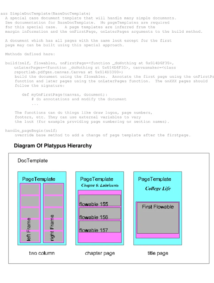
Document, page, paragraph and text layout are supported through a module named platypus, which stands for Page Layout and Typography Using Scripts. It works

by allowing definition of different containers, each with their own layout, which contains other, lower-level containers. With this organization, fine-grained control is allowed along with the ease of higher-level use. The highest level is

DocTemplate, which defines the way pages are arranged in the document, page borders and other page formatting, page transitions, etc.

BaseDocTemplate is usually the starting point for these, to which you must add a set of PageTemplates. PageTemplate is the next step lower – it is a very minimal container class which controls little formatting; its purpose is only to hold a list of frames. Frames are only used to separate blocks of the document into sections; they contain basic dimensions and padding. These three levels would allow you to for example:

◦ define your document contents by page content: ▪ perhaps a cover page as the first page:

 this page may contain a frame for a title, say limited to a center region, and other frames for other information. These would be collected in a cover page PageTemplate

▪ a table of contents page on the next page:

 this page could have a frame for title and frame for the table, collected into another PageTemplate. You may need the table of contents to 'flow over' to the next page – so long as the content is constrained to the same PageTemplate it will do so, and replicate the formatting from the previous page. PageTemplates also let you define behaviour such as drawing a title or repeating certain sections when

spanning multiple pages

▪ document content in other PageTemplates, each with their own frames

◦ the collection of PageTemplates, once you have them defined, is passed to the DocTemplate as a list.

(43)

(from reportlab.lib.units import inch) BaseDocTemplate(self, filename, pagesize=defaultPageSize, pageTemplates=[], showBoundary=0, leftMargin=inch, rightMargin=inch, topMargin=inch, bottomMargin=inch, allowSplitting=1, title=None, author=None, _pageBreakQuick=1, encrypt=None) BaseDocTemplate.addPageTemplates(self,pageTemplates) BaseDocTemplate.build(self, flowables, filename=None, canvasmaker=canvas.Canvas)

BaseDocTemplate event handlers: handle_currentFrame(self,fx) handle_documentBegin(self) handle_flowable(self,flowables) handle_frameBegin(self,*args) handle_frameEnd(self) handle_nextFrame(self,fx) handle_nextPageTemplate(self,pt) handle_pageBegin(self) handle_pageBreak(self) handle_pageEnd(self) PageTemplate(id=None,frames=[],onPage=_doNothing,onPageEnd=_doNothing) Frame(self, x1, y1, width, height, leftPadding=6, bottomPadding=6, rightPadding=6, topPadding=6, id=None, showBoundary=0,

overlapAttachedSpace=None, _debug=None) Frame.addFromList(drawlist, canvas) Frame.split(flowable,canv)

Frame.drawBoundary(canvas)

There is also a class named SimpleDocTemplate:

(44)

class SimpleDocTemplate(BaseDocTemplate)

| A special case document template that will handle many simple documents.

| See documentation for BaseDocTemplate. No pageTemplates are required

| for this special case. A page templates are inferred from the

| margin information and the onFirstPage, onLaterPages arguments to the build method.

|

| A document which has all pages with the same look except for the first

| page may can be built using this special approach.

|

| Methods defined here:

|

| build(self, flowables, onFirstPage=<function _doNothing at 0x014D6F30>,

onLaterPages=<function _doNothing at 0x014D6F30>, canvasmaker=<class

reportlab.pdfgen.canvas.Canvas at 0x014D3300>)

| build the document using the flowables. Annotate the first page using the onFirstPage

| function and later pages using the onLaterPages function. The onXXX pages should

| follow the signature:

|

| def myOnFirstPage(canvas, document):

| # do annotations and modify the document

| ...

|

| The functions can do things like draw logos, page numbers,

| footers, etc. They can use external variables to vary

| the look (for example providing page numbering or section names).

|

| handle_pageBegin(self)

| override base method to add a change of page template after the firstpage.

| override base method to add a change of page template after the firstpage. Diagram Of Platypus Hierarchy

(45)

Lower-level Control

At a lower level than these templates are a set of content objects called Flowables, and the pdfgen canvas. These are text or graphic elements which are 'flowed' into frames and fill the page. When the page is full, they begin flowing into the following page. Some flowables include:

Spacers:

import reportlab.platypus.Spacer Spacer(self, width, height)

Guaranteed gap between things

Paragraphs:

import reportlab.platypus.paragraph.Paragraph Paragraph(text, style, bulletText=None, caseSensitive=1)

Paragraphs are passed a content string which comprises their text, and a style argument, usually ParagraphStyle. The string argument can contain certain HTML-like XML tags to control their formatting.

import reportlab.lib.styles.ParagraphStyle

Images:

(Flowable image, there is also a Drawing/Shape Image) import reportlab.platypus.Image

Images(self, filename, width=None, height=None, kind='direct', mask='auto', lazy=1)

 If size to draw at not specified, gets it from the image.

Digital picture of any format supported by Python Imaging Library (PIL), centred horizontally within a Frame

Drawing/Shape Image is a more basic version for use with shapes: import reportlab.graphics.shapes.Image

(46)

Tables: import reportlab.platypus.Table Table(self, data, colWidths=None, rowHeights=None, style=None, repeatRows=0, repeatCols=0, splitByRow=1, emptyTableAction=None, ident=None, hAlign=None, vAlign=None)

Tables have 2 main parts along with their dimensions: their contents (data) and formatting (style) . Contents can be strings and integers, or another type of flowable, arranged in a list of lists. Widths and heights can be defined as a list containing tuples or None; if None it is spaced

automatically. hAlign/vAlign is alignment in parent document, one of the following strings: "LEFT", "RIGHT", “TOP”, “BOTTOM”, "CENTER", "CENTRE". Example of contents: data = [['00', '01', '02', '03', '04'], ['10', '11', '12', '13', '14'], ['20', '21', '22', '23', '24'], ['30', '31', '32', '33', '34']] Style: import reportlab.platypus.TableStyle

list of lists in following format, containing one of following arguments:

['VALUE',(startCol,startRow), (endCol,endRow), [numberArg], [keyWordArg]]

FONT - takes fontname, optional fontsize and optional leading. FONTNAME (or FACE) - takes fontname.

FONTSIZE (or SIZE) - takes fontsize in points; leading may get out of sync.

LEADING - takes leading in points.

TEXTCOLOR - takes a color name or (R,G,B) tuple.

(47)

CENTER) or DECIMAL.

LEFTPADDING - takes an integer, defaults to 6. RIGHTPADDING - takes an integer, defaults to 6. BOTTOMPADDING - takes an integer, defaults to 3. TOPPADDING - takes an integer, defaults to 3. BACKGROUND - takes a color.

ROWBACKGROUNDS - takes a list of colors to be used cyclically. COLBACKGROUNDS - takes a list of colors to be used cyclically. VALIGN - takes one of TOP, MIDDLE or the default BOTTOM

SPAN – merges cells bounded by (startCol,startRow), (endCol,endRow) ex: style = TableStyle( [('LINEABOVE', (0,0), (-1,0), 2, colors.green), ('LINEABOVE', (0,1), (-1,-1), 0.25, colors.black), ('LINEBELOW', (0,-1), (-1,-1), 2, colors.green), ('ALIGN', (1,1), (-1,-1), 'RIGHT')] ) Drawings: import reportlab.graphics.shapes.Drawing Drawing(self, width=400, height=200, *nodes, **keywords)

A container for shapes, usually instance assigned to a variable, then shapes or widgets are added to it. Allows conversion to objects from other classes and inherits transformation methods of Group.

Methods:

asGroup(self, *args, **kw)

asString(self, format, verbose=None, preview=0, **kw) copy(self)

resized(self, kind='fit', lpad=0, rpad=0, bpad=0, tpad=0) save(self, formats=None, verbose=None, fnRoot=None,

outDir=None, title='', **kw)

wrap(self, availWidth, availHeight) Methods inherited from Group:

add(self, node, name=None) asDrawing(self, width, height) getBounds(self) getContents(self) insert(self, i, n, name=None) rotate(self, theta) scale(self, sx, sy) shift(self, x, y) skew(self, kx, ky) translate(self, dx, dy)

(48)

Methods inherited from Shape:

__setattr__(self, attr, value) dumpProperties(self, prefix='') getProperties(self, recur=1) setProperties(self, props) verify(self) Strings: import reportlab.graphics.shapes.String String(self, x, y, text, **kw)

Basic string, can be placed with coordinates, can be convenient where a Paragraph is cumbersome. Can be anchored left, middle or end.

Groups:

import reportlab.graphics.shapes.Group

Allows you to group a bunch of shapes together, but operates on a lower level than Drawing. Allows for basic transformations

Methods:

add(self, node, name=None) asDrawing(self, width, height) copy(self) getBounds(self) getContents(self) insert(self, i, n, name=None) rotate(self, theta) scale(self, sx, sy) shift(self, x, y) skew(self, kx, ky) translate(self, dx, dy) Shapes:

from reportlab.graphics.shapes import ArcPath, Circle, Ellipse, Line, Path, PolyLine, Polygon, Rect, Wedge Many generic shapes, they are generally straightforward:

ArcPath(self, points=None, operators=None, isClipPath=0, **kw)

Path with an addArc method inherits Path()

Method:

(49)

centery, radius, startangledegrees, endangledegrees, yradius=None, degreedelta=None, moveTo=None, reverse=None) Circle(self, cx, cy, r, **kw)

Ellipse(self, cx, cy, rx, ry, **kw) Line(self, x1, y1, x2, y2, **kw)

Path(self, points=None, operators=None, isClipPath=0, **kw)

Path, made up of straight lines and bezier curves. Methods:

closePath(self) copy(self)

curveTo(self, x1, y1, x2, y2, x3, y3) getBounds(self)

lineTo(self, x, y) moveTo(self, x, y)

PolyLine(self, points=[], **kw)

Series of line segments. Does not define a closed shape; never filled even if apparently joined. Put the numbers in the list, not two-tuples.

Polygon(self, points=[], **kw)

Defines a closed shape; Is implicitly joined back to the start for you.

Rect(self, x, y, width, height, rx=0, ry=0, **kw)

Rectangle, has rounded corners if radius arguments set

Wedge(self, centerx, centery, radius, startangledegrees, endangledegrees, yradius=None)

A "slice of a pie" by default translates to a polygon moves anticlockwise from start angle to end angle

Charts And Widgets:

(50)

widgetbase.py and are essentially drawings with methods. In version 2.4 of ReportLab samples can be found in Python26 \ Lib \ site packages \ reportlab \ graphics \ samples, wherever you installed python. The runall.py module runs them all in a batch. More can be found in the graphics directory and on the reportlab website. Charts are built from from sub-modules found within the graphics directory which can be used on their own to create various useful objects such as grids, labels, axes, etc. Many charts are available and the best resource to consult would be the Graphics portion of the user guide, coupled with Windows Grep and the source code itself (most objects have convenient

getProperties() and .dumpProperties() methods which let you see a list of

available attributes; these are usually defined using AttrMapValue(). These things together provide great documentation) It is an area of development in ReportLab, so much of the documentation, and I would imagine even underlying structure will be further refined in the future.

A Note On Coordinates:

Coordinate in ReportLab are only standard if you happen to have chosen the right standard as your base. Generally numerical coordinates are Cartesian, and place the origin at bottom/left rather than the top/left portion of a page we might expect

A Note On Formatting:

Formatting in ReportLab follows the ques from the lowest-level for which

formatting has been defined, generally attempting to override higher-levels. If a single part of the formatting is defined at a level, make sure the rest of the content is handled appropriately, for example, I encountered problems with font types at times because I defined certain specific low-level formatting options and it caused the rest of the formatting at that level to revert to default arguments.

PDFGEN:

The lowest level available in ReportLab, this module allows for rendering any of the objects defined in reportlab.graphics.shapes (or within the rendering packages themselves) directly to the PDF canvas (construct which allows coordinate placement of visual objects (text, shapes, images, etc.) onto a space, written to the blank part of an empty pdf. Drawing is similar to the way a graph is plotted, where the canvas is a graph with hidden axes and many of the mathematical constructs are wrapped in higher-level language) When this vector image is created it can be drawn directly using a number of renderers into many formats. ReportLab at present, includes the following renderers:

(51)

renderPDF.

default renderer. As with the others, it can be used directly by calling it's draw method. This allows direct drawing to an appropriately-sized pdf without the need to define some sort of document.

renderPM

Used for Pixel Map images such as .gif, .tif, .png, .bmp, .ppn, .jpg, .pct, PIL etc. Can create files, or buffer images for

output to another system.

renderPS

similar to others, but used for PostScript and eps support

renderSVG

used for Scalable Vector Graphics, .svg files

These are also useful in that they can override the platypus module and draw directly on the .pdf independently: this is usually how one would place a header, footer, perhaps page numbers, etc: other things which are not dependant on other page content. In development at time of writing is support for importing these various formats into ReportLab so they do not need to be recreated if you're pulling them out of another source, say, a module of matplotlib, or wish to place a vector image into your file, but you wouldn't need to convert to a raster/scalar image format and lose image quality or the ability to edit the file in another software package such as Inkscape or OpenOffice.org Draw.

(52)

Sample Code

Here's an example of some code which uses reportlab:

import reportlab

# main module

from reportlab.lib.units import inch

from reportlab.lib import colors

from reportlab.graphics.shapes import Drawing, Rect, Image

from reportlab.graphics.charts.lineplots import

ScatterPlot

from reportlab.graphics import renderPDF

#^^ Portable Document Format renderer; handles .pdf

from reportlab.graphics import renderPS

#^^ PostScript renderer; handles .ps, .eps, etc.

from reportlab.graphics import renderPM

#^^ PixMap renderer

# handles .gif,.tif,.png,.bmp,.ppn,.jpg,.pct,PIL etc.

from reportlab.graphics import renderSVG

#^^ Scalable Vector Graphic renderer; handles .svg

import headerfooter

# module which creates a letter-size pdf document, draws a header

# and footer onto each page and fills the space between with

# flowables

from formatting import fixFormatting

# applies a property set for charts, fills them with data

drawing = Drawing(width=72*6, height=72*8)

# creates a Drawing object to which we add things

# create objects to add to drawing and eventually draw to page:

rectangle = Rect(x = 1.5*inch, y = 6*inch, width = 300, height = 100,

(53)

fillColor = colors.darkorange)

logo = Image(x = .5*inch, y = 6*inch, width = 50, height = 30, path = r'NRC.jpg') chart = ScatterPlot() fixFormatting(chart)

# add the object to the drawing:

drawing.add(rectangle)

drawing.add(logo)

drawing.add(chart)

# pass it to the module which will draw it to pdf

headerfooter.PageTitle = "Presentation Demo" headerfooter.pageContent(drawing)

# for the sake of doing it, create some images containing our

# objects

renderPS.drawToFile(drawing, 'demo.eps')

(54)

(55)

APPENDIX E

(56)

iceSheetSummaryPDF.py

current content/workings:

 imports

 initializing a few global variables  database connection using pymssql

 aliasing of content fetched from database to local variables, should be reviewed by tank operators / Brian Hill

 definition of unit functions which wrap a received value in a paragraph in order to give it the right unit and formatting when displayed in table flowable  functions which draw default header and footer,

surrounding each are functions which define non-standard, but useful headers and footers: this should all be relegated to headerfooter.py passed the variables they require, along with flags to select proper header/footer type and applied there  definition of two functions which

SimpleDocTemplate requires for first page and later page page layout; they only tell the doc to draw the header and footer on each page and would not be necessary if headerfooter.py handled the page layout

 definition of the main() function, named go(), called at the bottom of the file if the file is being tested as a standalone, and not run or imported from another file (in the case where it is invoked on its own, the value of __name__ is '__main__', in other cases it is the name of the script.

 'go()' consists of:

◦ a ParagraphStyle() instance , style, is defined, this is used as the default throughout the file.

◦ A list variable is defined for the 'data' argument of each table on the sheet. Each of these variables contains a list for each row in that table with an element for each column. Elements in the inner list contain Paragraphs for formatting, and unit function calls to wrap up values with their

associated units. There is probably a cleaner way of doing it; this way seemed compact but legible. ◦ A common style is defined for the tables: they

(57)

will all look the same

◦ the document object is created, along with a Spacer() flowable to which the content of the doc is added, the document 'built', and then

launched.

data required + format:

 at the moment, no data extra is required because it fetches all it needs from a view

(vwIceSheetSummary)

 the SQL string which is used could be relegated to sqlstatements.py for consistency

 this data is aliased near the top and were it to be done differently, this would provide a pretty good spec of 'what is required'

 the values that are being read should be reviewed by an expert to be sure what is being displayed is

actually as the titles advertise on the final product.

what it 'should' look like

 this script should only contain only the processing of flowables, so that they can be passed into another file which produces the document, along with relevant settings. The rest of the machinery could be placed elsewhere. This is the basic idea behind what all these scripts 'should' look like

mechanicalPropertiesSummaryPDF.py current content/workings:

 This file basically requires the contents of a .LOG file, assigned to the proper variables: groups of summary values for each test, in chronological order. It reads in this object, expecting it to be formatted as a list of dictionaries (very similar to DatabaseTable() objects or C# DataTables, with each row in the table being a summary for a particular test, and all the rows ordered by times the tests were taken) looks for "Test Type" flags, given the value of the flag it loads a set of keys for that type, uses all the keys to append the values to an internal Table() data variable in a specific order, append certain

TableStyle tags to another internal variable, create a Table() object, and pass it the 2 variables which will comprise its contents (data) and

(58)

table which shows test results over time

 file begins with some imports, looks up IceSheetId  next are lists of the keys required for each test: values

for each of these MUST be passed to the file when processing a test of that type. Sample values and descriptions which go with these keys can be found in datatable.py; it gets used to pull dummy data.  After listing the keys it randomly generates a dummy

object which has all the right keys and similar-looking values using what is finds in datatable.py. Being unordered/random they aren't sequenced by time (in reasonable probability).

 Next values for the header and footer are fetched from the database using sqlstatements.py to get the SQL query string, and sqltables.py to fetch the values. These are then aliased. They should at this point be passed to headerfooter.py but this file, like iceSheetSummaryPDF.py takes care of its header and footer internally.

 Next some variables are created for the ReportLab part:

◦ style for paragraphs

◦ Story to hold the list of flowables ◦ tableTitle for the main table ◦ colTitles for its column names

◦ rowNumber is the number for the first row to which we will begin appending data, it is 2 because the first 2 rows of of our main table will be taken up by titles. Also, the first 2 rows get repeated in the event of a page transition to repeat the titles; you wouldn't want the titles to be numbers instead

 a PDF document is created: it should be ReportLab handling document creation, with just the variables left in this file to create an object to be passed to

headerfooter.py

 more variables are created for the ReportLab part: ◦ tableStyleArg to format the title rows of the

table

◦ tableContent to hold all the data we'll be appending to our table, we start it with the titles rows, sequentially piping the 2 list variables we