Bayesian Inference Algorithm on Raw by
Alda Luong
Submitted to the Department of Electrical Engineering and Computer Science in Partial Fulfillment of the Requirements for the Degree of Master of Engineering in Electrical
Engineering and Computer Science at the Massachusetts Institute of Technology
August, 2004 a - t04
0 Massachusetts Institute of Technology. All rights reserved.
The author hereby grants to M.I.T. permission to reproduce and distribute publicly paper and electronic copies of this thesis and to grant others the right to do so.
Author Certified by Certified by ,. Certified by Accepted by MASSACHUSETTS INSTIT OF TECHNOLOGY
JUL 18 2005
LIBRARIES
10Department of Electrical Engineering and Computer Science
A
A August 24, 2004 Anant Agarwal Thesis Advisor Eugene Weinstein Co-Thesis Advisor . I /' James LebakJf-y incoln Laborpo visor
Arthur C. Smith Chairman, Department Committee on Graduate Theses
BUTE BARKER
Bayesian Inference Algorithm on Raw
by
Alda Luong
Submitted to the Department of Electrical Engineering and Computer Science on August 24, 2004, in partial fulfillment of the
requirements for the degree of
Master of Engineering in Electrical Engineering and Computer Science
Abstract
This work explores the performance of Raw, a parallel hardware platform developed at MIT, running a Bayesian inference algorithm. Motivation for examining this parallel system is a growing interest in creating a self-learning and cognitive processor, which these hardware and software components can potentially produce. The Bayesian
inference algorithm is mapped onto Raw in a variety of ways to try to account for the fact that different implementations give different processor performance. Results for the processor performance, determined by looking at a wide variety of metrics look promising, suggesting that Raw has the potential to successfully run such algorithms.
Acknowledgements
I would like to give special thanks to Eugene Weinstein, my campus co-thesis advisor, for helping me with all aspects of the project. Not only did Eugene give me general guidance on the project, but he also contributed to the nitty-gritty aspects of it like debugging code and writing scripts for data conversions. I also want to thank him for being so readily available to help, especially during the last few weeks of the project
when he was on call for any questions I had.
I would like to thank Janice McMahon, my Lincoln Laboratory thesis advisor, for giving me direction and goals in the project, making sure I was on the right track, and encouraging me along the way.
I would like to thank James Lebak, my other Lincoln Laboratory thesis advisor, and Robert Bond, Lincoln Lab Embedded System group leader, for being supportive and giving me many great ideas and guidance.
Thanks also go out to my other on-campus advisor, Anant Agarwal. Although he was incredibly busy, he took time out to give me direction in the project and to help me out with parallel processing concepts.
Much thanks to my Lincoln Lab co-workers, Henry Hoffman, who helped with questions on Raw, and Nadya Travinin, who helped me understand Bayesian networks and inference algorithm concepts.
I would like to thank Karen Livescu of the Spoken Language Systems Group for letting me borrow her speech recognition dynamic Bayesian network to map onto Raw and for answering my many questions regarding her application.
Last, but not least, I would like to thank my family and friends for being so supportive and understanding. Special thanks to my mom who knew how stressed out I was and took care of my other life worries as I worked on this project.
Contents
1. Introduction ... 5
1.1 M otivation... 5
1.2 Objectives ... 6
1.3 Organization and Content of the Text... 6
2. Parallel Hardw are Platform ... 8
2.1 Trend in Current Technology... 8
2.2 Problem s w ith Current M icroprocessors ... 10
2.3 Approach to Current M icroprocessor Problem s ... 12
2.4 Parallel Architectures... 13
3. Application... 19
3.1 Bayesian N etworks and Inference Algorithm s ... 19
3.2 Feature-Based Pronunciation Model for Speech Recognition... 27
4. Parallel System Analysis... 31
4.1 Perform ance M etrics... 31
4.2 Sources of Overhead ... 33
5. Im plem entation of Application... 34
5.1 A lgorithm ... 34
5.2 M apping ... 36
6. Results... 41
7. Conclusion ... 47
Appendix A: Frames in Feature-based Pronunciation Model... 49
Appendix B: Fine Grain Parallelization... 52
Appendix C: Code for Particle Filtering Algorithm ... 54
1.
Introduction
1.1 MotivationThe idea of creating a "cognitive" processor, which is loosely defined as a machine that can think and learn from its environment, has been a recent research endeavor. This sort of self-sufficient processor could address a wide body of needs in industry as well in the military. Hi-tech companies, for example, have been pushing for products that are
self-learning and self-organizing for search technologies. The military has been turning to intelligent processors for use in resource management, unmanned system mission planning, intelligence analyst assistance, and unattended ground sensors data fusion, interpretation, and exploration.
Choosing the appropriate algorithm that can perform "cognition" as well as the architecture that would best support the software is still under speculation and study. Statistical learning models, such as Bayesian Networks, Learning Decision Trees, Support Vector Machines, and Nearest Neighbor are potential algorithms since they can perform reasoning. Scalable computer architectures such as the Raw chip developed at MIT, the Smart Memories chip developed at Stanford, or the IRAM developed at U.C. Berkeley, are likely candidates for the processor since their large I/O bandwidth, flexibility, and capability of parallel processing potentially match the requirements of these learning algorithms. Since research in this field is still new, not much is known of the compatibility of these hardware and software components. This thesis project hopes to broaden understanding in this area.
1.2 Objectives
A parallel system, which is the combination of an algorithm and the parallel architecture on which it is implemented, will be studied in this work. The primarily goal of the analysis is to determine the weaknesses and strengths of the hardware platform, and to decide on the best parallelization of the algorithm. For this project, the parallel system is comprised of a Bayesian inference algorithm running on the Raw microprocessor. The Bayesian inference algorithm is chosen because of its wide use and popularity in the artificial intelligence community and the Raw architecture is used because of its accessibility to MIT researchers.
The primary challenge of this project is parallelizing the inference algorithm to be used on the microprocessor. This "mapping" process involves breaking the serial
algorithm into smaller pieces of code to be run in parallel on the hardware platform. For this study, the algorithm is mapped in a number of ways that cover varieties of
communication patterns and data dependencies. This is to account for the fact that different mappings produce different performance results. The parallel system
performance is then examined and evaluated using numerous metrics described in section 4.
1.3 Organization and Content of the Text
This paper delves into two major field of study: parallel computer architectures and Bayesian inference algorithms. The text is organized as follows:
This section tries to provide an understanding of the evolution and need for parallel architectures in the next generation of microprocessors. Particular examples of parallel processors that will be looked at, include MIT's Raw, Stanford's Smart Memories, and U.C. Berkeley's Vector IRAM.
3. Application
Background information on Bayesian networks and inference algorithms will be discussed extensively, along with a description of the feature-based pronunciation modeling for speech recognition application that will be mapped onto the chip.
4. Parallel System Analysis
This section will discuss a variety of metrics used to measure the performance of the parallel system.
5. Implementation of Application
The code implementation and mapping procedure of the Bayesian inference algorithm will be addressed in this section.
6. Result
Performance results of the parallel system are presented and interpreted in this section. Metrics used in this analysis include those discussed in section 4.
7. Conclusion
This section reexamines the performance of the parallel system and discusses the compatibility of the Bayesian inference algorithm and the Raw microprocessor.
2.
Parallel Hardware Platform
MIT's Raw microprocessor serves as the parallel hardware platform in this project. Raw is a scalable, highly parallel processor that is predicted to replace future microprocessors. Background information on Raw and motivation for the development of this sort of processor, is described in the following sections.
2.1 Trend in Current Technology
The ongoing trend in microarchitecture research is to design a microprocessor that can accomplish a group of tasks or applications in the shortest amount of time while using minimum amount of power and incurring the least amount of cost [16]. In terms of these metrics, microprocessor technology has experienced tremendous performance gains over the past decade. These advances have been made possible by improvements in a variety of disciplines, of which process technology and microarchitecture enhancements have been most significant [16].
Fabrication Process Technology
Fabrication process technology is considered the main driving force of the
microprocessor industry, having a direct impact on the speed, cost-efficiency, and performance of devices. Developments in lithography and etching techniques, for example, reduce feature sizes of transistors. Improvements in materials technology have allowed the integration of more and more devices on a single die, resulting to an increase in circuit device packing density [17]. Furthermore, an increase in die size has led to an increase of chip complexity and, therefore, computation capabilities of devices. This
trend has been the driving force of Moore's Law, which states that every 18 months the rate of circuit complexity doubles (extrapolated in 1965) [7].
The phenomenon of increasing chip density/complexity has become apparent in the miniaturization of microprocessors. In 1987 a microprocessor containing about 100,000 transistors could fit on one square centimeter of silicon. In 1997, the same microprocessor could fit on one millimeter square. It is projected that in 2007, such microprocessor would be able to fit onto a chip one-tenth of a millimeter [2]. In 2001 the Semiconductor Industry Association (SIA) predicted that by 2011, industry would be manufacturing 1.5 billion-transistor processors with clock speeds over 11 GHz [3]. Undoubtedly, immense computation capabilities have been made possible with this growth in chip complexity.
Microarchitecture
Enhancements in current microarchitectures have helped realize logic functions more effectively, therefore increasing microprocessor performance. Microarchitecture affects performance by reducing the frequency of the clock and instructions executed per clock cycle, in which performance is characterized by the following relationship: Performance
=1/Execution Time = (Instruction Per Cycle x Frequency)/Instruction Count. Enhancements to microarchitectures, mostly in the form of instruction-level
parallelization, can reduce the amount of work done in each clock cycle, thus shortening the clock cycle [7].
One of these architectural enhancements includes pipelining, which breaks the processing of an instruction into a sequence of operations or stages. A new instruction
enters a stage as soon as the previous one completes that stage. A pipelined
microprocessor with N pipeline stages can ideally deliver N times the performance of one that is unpipelined. Superscalar execution is another widely used architectural
improvement, in which the number of instructions per cycle can be reduced by executing several instructions in parallel. In this implementation, two or more instructions can be at the same pipe stage at the same cycle. A major problem with superscalar execution is that significant replication of resources are required. Out-of-order execution is an architecture feature that can also increase performance by increasing the number of instructions per cycle. In out-of-order execution instruction, execution order is dependent on data flow instead of the program order. This sort of implementation involves dependency analysis and instruction scheduling, which means that more clock cycles need to be committed to process an instruction out-of-order [9].
2.2 Problems with Current Microprocessors
With the tremendous technological advances recently, researchers have been finding it harder and harder to keep up this pace. Power and communication delay and processor performance improvements are becoming limiting factors in microprocessor design. The rate at which data can be accessed from memory (bandwidth) has been another major concern.
Despite the fact that transistor switching delay has become shorter, growing chip complexity has contributed to the slowing down of processing time as well as power inefficiency. The root of these problems lies in wires. Most of the area of a chip is covered with wires on several levels (transistor switches rarely take more than about 5
percent of the area on the lowest level) [12]. The trend for increasing die size worsens this case since interconnect wires are proportional to the die size. These long, overlapping wires contribute to capacitive coupling, which is the transfer of energy from one part of a
circuit to another, causing significant signal delays. It is predicted in 2010 that sending signals across a billion-transistor processor may require as many as 20 cycles, making it impossible to maintain a global clock over the entire chip [5]. Furthermore, these longer wires require more power to drive, leading to a greater power strain.
The demand for greater performance, achieved by increasing frequency, has had an impact on power as well. More power is naturally used up for processors operating at higher frequencies. It is predicted that the higher frequency, coupled with increased device density, would raise power usage to a level that cannot suite mobile computers. Increasing performance by increasing the number of instructions per cycle would, therefore, be more energy efficient.
Another issue that has emerged is the ability of the memory system to feed data to the processor at the required rate. As performance demands increases, bottlenecks are posed by the datapath and the memory'. Clock rates of high-end processors have increased at roughly 40% per year over the past decade, DRAM access times have only improved at the rate of roughly 10% per year over this interval [16]. Coupled with increases in instructions executed per clock cycle, there is a growing gap between processor speed and memory. Although this problem can be alleviated by creating memory hierarchy of successively faster memory, called caches, performance improvements are still limited.
2.3 Approach to Current Microprocessor Problems
One of the main problems with the current microprocessor trend is that chip architecture and technological advancements introduce few significant design changes - that is, microprocessors that are being built today are more complex versions of those that have already been built [2]. As a result, communication costs, power inefficiency, and memory latency will continue to grow, setting a limit on microprocessor performance. Evidently, microprocessor technology is approaching a wall.
In response to these growing concerns, research to solve microprocessor trend problems has focused on parallel computing technologies. Multiprocessor solutions have contributed to the acceleration of computing elements by providing multiplicity of data paths, increased access to storage elements, scalable performance, lower costs, and lower power consumption. An example is the on-chip multiprocessor, which is comprised of a number of processors occupying a single die. Better memory system performance is achieved because on-chip multiprocessors provide larger aggregate caches and higher
aggregate bandwidth to the memory system than that of a typical microprocessor [7]. Consolidating an entire instruction processor onto a single chip together with as much of the lowest levels of the storage hierarchy (i.e., registers, stack frames, and instruction and
data caches) as possible reduces communication lengths and, therefore, delays. Power efficiency is also indirectly impacted by these multiprocessor machines. Power in a microprocessor system is usually used up by driving capacitive loads. In multiprocessors, power per device scales down quadratically while the density scales up quadratically, so that the power per unit area need not be increased over today's levels. Perhaps the most important advantage of the on-chip multiprocessor is its ability to scale. Since
components on a multiprocessor chip have uniform, modular computing units, performance or speedup can be maintained with increasing number of processors.
2.4 Parallel Architectures
Because microprocessors are predicted to approach a billion transistors within the next decade, researchers are posed with the problem of how to best utilize this great resource.
This predicament is known as the "billion transistor" dilemma. A prevailing response has been to shift traditional microprocessor structures to parallel architectures so that
modularity, reconfigurability, and scalability can be achieved. A discussion of a sample of three leading parallel architectures, which include Stanford's Smart Memories, MIT's Raw, and U.C. Berkeley Vector IRAM follows below. Descriptions will focus on benefits of the new architecture, memory systems, and types of interconnect networks. Although only Raw is used in this project, the two other hardware platforms have great potential in future computer architecture development and will help in understanding the weaknesses and strengths of Raw.
Raw
Raw is the first tiled architecture to be fabricated and was developed at MIT Laboratory of Computer Science, under the auspices of Professor Anant Agarwal in the Computer Architecture Group. Raw is composed of a 2-dimensional array of identical,
interconnected tiles. Each tile is comprised of a main and switch processor, and a dynamic router. The main processor performs all computation on the tile, whereas the switch processor and dynamic router are responsible for communication among the tiles.
The modular nature of the design ensures that wire lengths shrink as technologies improve, allowing wire and gate delays to scale at roughly the same rate. The multiple processing elements take advantage of both instruction-level and thread-level parallelism
[8].
The main processor on each tile (also known as the "tile processor") has a 32 kilobyte SRAM data memory, a 32 kilobyte instruction memory, a 32-bit pipelined FPU, a 32-bit MIPS-style compute processor, and routers and wires for three on-chip mesh networks. The switch processor has a local 8096-instruction memory, but no data memory. A diagram of the tile is shown in figure 7.
Switch Memory (8k x 64) Partial Crossbar Switch Processor FPU Processor
Instruction Data Memory
Memory 4k x 64)
(8k x 32)
Figure 7: Components of a Raw Tile
The tile processor uses a 32-bit MIPS instruction set, with some slight
modifications [13]. The switch processor, which controls the static network, also uses a
MIPS instruction set, but stripped down to four instructions (nops, moves, branches, and jumps). Each MIPS instruction is read alongside a routing component, which specifies the direction of the data transmission. Similar to the switch processor, the dynamic router, which controls the dynamic network, runs independently of the main processor but, in contrast, the user has no direct control over the dynamic router. In a dynamic send, users specify the destination tile of data in the main processor code. The tile processor is able to communicate with the switch through three ports (two inputs and one output) and the dynamic router through four ports (two inputs and two outputs).
Many features of Raw make the microprocessor flexible and potentially high performing. Exposing hardware detail to software enables the program or compiler to make decisions on resource allocation and, therefore, achieve greater efficiency. Fine-grain communication between replicated processing elements exploits huge amounts of parallelism in applications. Also, the rigid, tiled structure of the Raw chip allows for wire
efficiency and scalability since data paths cannot extend beyond the length of a single tile.
Smart Memories
A Smart Memories chip, which is under development at Stanford University, is similar to Raw. It is a tiled architecture and is made up of many processing tiles, each containing
local memory, local interconnect, and a processor core. For efficient computation under a wide class of possible applications, the memories, the wires, and the computational model can all be altered to match the applications [13].
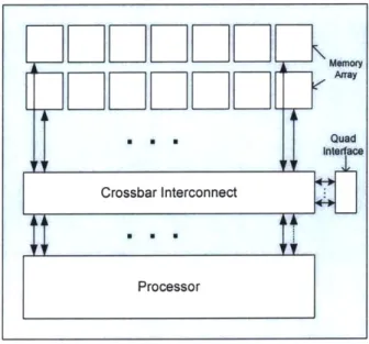
The Smart Memories chip is comprised of a mesh of tiles in which every four processors are grouped into units called "quads." The quads communicate via a packet-based, dynamically-routed network. Each tile, shown in figure 1, is comprised of a reconfigurable memory system, a crossbar interconnection network, a processor core, and a quad network interface.
Memory
DDDLJ[]
Array
* * .Quad Into ace Crossbar Interconnect ProcessorFigure 1: A Smart Memories Tile
The key feature of the Smart Memories lies in the tile reconfigurable memory system. The 128 KB DRAM memories are broken up into small 8 KB chunks, called mats. The memory array has configurable logic in the address and data path, which allow
Smart Memories mats to be configured to implement a wide variety of caches, or to serve as local scratchpad memories or as vector/stream register files. To connect the different memory mats to the desired processor or quad interface port, the tile contains a
The processor of a Smart Memories tile is a 64-bit processing engine with
reconfigurable instruction format/decode. The computation resources of the tile consist of two integer clusters and one floating point cluster.
The main benefit of the Smart Memories chip is that breaking up the memory components into smaller pieces increases the memory bandwidth and decreases memory latency. Also, multiple processing elements take advantage of instruction-level and thread-level parallelism.
IRAM
The intelligent RAM (IRAM) is currently being researched at U.C. Berkeley. It is based on the idea of using on-chip space for dynamic RAM (DRAM) memory instead of SRAM caches. Because DRAM can accommodate 30 to 50 times more data than the same chip area devoted to caches, the on-chip memory can be treated as main memory. This sort of implementation appeals to processor designs that demand fast or frequent memory access. A machine that currently uses IRAM is the U.C. Berkeley vector processor, seen in figure 2.
Memory crossbar
7etiL U iftCaches T 0
Memory cross
Figure 2: Vector IRAM
The vector processor consists of a vector execution unit combined with a fast in-order scalar core. The combination of the vector unit with the scalar processor creates a general purpose architecture that can deliver high performance without the issue
complexity of superscalar designs or the compiler complexity of VLIW [11]. The vector unit consists of two load, one store, and two arithmetic units, each with eight 64-bit pipelines running at 1 GHz. The scalar core of the V-IRAM is a dual-issue processor with first-level instruction and data caches. The on-chip memory system has a total capacity of 96 Mbytes and is organized as 32 sections, each comprising of 16 1.5-Mbit banks and an appropriate cross-bar switch.
Because of the simplicity of circuits, vector processors can operate at higher clock speeds than other architectural alternatives. Simpler logic, higher code density, and the ability to selectively activate the vector and scalar units when necessary also provide higher energy efficiency [11]. Higher cost efficiency can also be achieved. Because the design is highly regular with only a few unique pieces used repeatedly across the die, the
development cost of V-IRAM can be much lower than it would be for other high density chips.
3.
Application
The Feature-Based Pronunciation Modeling for Speech Recognition, developed by Karen Livescu and James Glass of the MIT Computer Science and Artificial Intelligence
Laboratory, is used in this thesis project. This specific application is chosen because the Bayesian network associated with it is complex and shows a variety of communication patterns, making its mapping onto Raw interesting. The application and relevant background information are described in the following sections.
3.1 Bayesian Networks and Inference Algorithms
Bayesian networks and inference algorithms are used by the feature-based speech recognition application and are described in depth in this section.
Bayesian Networks
Bayesian networks (also known as Belief networks, causal networks, probabilistic networks, and knowledge maps) are data structures that efficiently model uncertain knowledge in complex domains. More specifically, Bayesian networks are
representations of joint probability distributions and consist of the following components: * A set of variables, in which each variable can be discrete or continuous. Discrete
variables have a finite set of mutually exclusive states. Continuous variables, which are most often represented using a linear Gaussian model, have an
unlimited range of representations. Each variable also has the property of being observed or unobserved, in which its state is known or not known. The value of the known state of an observed variable is that variable's evidence.
0 A set of directed edges between variables. The directed edges, along with the variables, together create a directed acyclic graph (DAG). Each node (or variable) in the DAG is conditionally independent of its predecessors in the node ordering, given its parents.
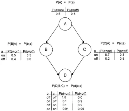
* A conditional probability table (CPT) attached to each variable. The CPT expresses the potential P(AIB1, ...,B,) of the variable A, with direct parents B1,...,B,. The probabilistic value of node A is unaffected by its non-descendents. Figure 3 shows an example of a Bayesian network containing four discrete random variables (A, B, C, D). Each variable is discrete and has two states (on or off).
P(BIA) = P(bla) a IP(b=on) IP(b=o on 10.5 0.5 off 0.4 0.6 P(A) = P(a) P(a=on) P(a=off) 0.5 0.5 A B C C on off D P(DIB,C) = P(dlb,c) b c P(d=on) P(d=off) off off 1.0 0.0 on off 0.1 0.9 off on 0.1 0.9 on on 0.01 0.99
Figure 3: Bayesian Network
P(CIA) = P(cla)
P(a=on) P(a=offD 0.7 0.3
The full joint probability, which is the collection of probability values
representing a complete stochastic system, can be derived from the CPT values by using the Bayesian chain rule. Derivation for the chain rule is as follows (lower case letters represent variables and upper case letter represent particular instances of a variable):
" A joint probability can be written in terms of conditional probability using the product rule:
P(x x P(x x x I )P(x x(1)
" Each conjunctive probability is reduced to a conditional probability and a smaller conjunction:
P(x I,..., x11)= P(xII I xn1 ,..., x1 )P(xn I xn-2 , ... , x) ... P(X2 I XI)P(XI)
= P (xi x i -1,...,x,) (2)
" The conditional probabilities can be simplified using conditional independence relationships. It can be seen that each entry in the joint distribution is represented by the product of the appropriate elements in the conditional probability tables in the Bayesian network [15]:
* The identity can be extended to hold for any set of random variables. This establishes the Bayesian network chain rule:
P(X,,..., X)=
1
P(Xi I parents(X)) (4)1=1
The Bayesian network derives its modeling power from the fact that every entry in the full joint probability distribution can be calculated by simply taking the product of the appropriate CPT values in the network. This can drastically reduce the amount of data needed to represent a stochastic system since Bayesian network CPTs take advantage of conditional independence and collectively require fewer values to represent then a complete joint probability table. To illustrate this, let us look at a stochastic system with 20 random variables. If each random variable can have 2 states, then a total of 220 table entries are required to represent the system. However, in a Bayesian network, if each random variable has a maximum average of 10 parents (this value is restricted by the DAG property), then only 20*210 values are needed to represent the system.
The network in the above example is a static Bayesian network and only represents a single stochastic event. Bayesian networks can also represent stochastic processes, in which a series of probabilistic events are generated over time. The temporal model comes in the form of a dynamic Bayesian network (DBN). A DBN network is comprised of repeated multiple static Bayesian networks connected to one another by directed edges. Each static network represents a time slice and the directed edges represent the forward flow of time. Hidden Markov models (HMM) and linear dynamic
Bayesian Inference Algorithms
Bayesian networks are most often used for probabilistic inferences. The basic task for any probabilistic inference system is to compute the posterior probability distribution for a set of query variables, given some observed event. A typical query asks for the posterior probability distribution P(X
I
e), in which X denotes the query variable and e is a particular observed event [15].Inferences can be exact or approximate. Two major classes of exact inferences include enumeration and clustering algorithms. In enumeration, a query is produced by computing sums of products of conditional probabilities from the network. In clustering algorithms polytree networks are formed for making large queries using a special-purpose inference algorithm called the Probability Propagation in Trees of Clusters algorithm (PPTC) [15]. Approximation methods are used to avoid exponential complexity in exact inferences. Classes of approximate inferences include direct sampling methods and Markov Chain Monte Carlo (MCMC). In direct sampling methods, random sampling processes generate events from a Bayesian network. In MCMC, events are generated by making random changes to the preceding events.
Particle Filtering Algorithm
This project will involve the use of the likelihood-weighting method (also known as the particle filtering method). It is chosen for its algorithmic simplicity and potential to be parallelized.
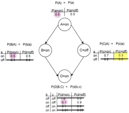
Particle filtering is a form of direct sampling for networks with evidence. This method utilizes a large number2 N of random samples (or particles) to represent the posterior probability distributions [4]. In likelihood-weighting, values for the evidence variables E are fixed, and only the remaining variables are sampled. This guarantees that each event is consistent with the evidence. Not all events are equal, however. Before tallying the counts in the distribution for the query variable, each event is weighted by the likelihood that the event accords to the evidence, as measured by the product of the conditional probabilities for each evidence variable, given its parents [15]. The following example goes through all stages of particle filtering algorithm for the Bayesian network shown in figure 3. In this case, four particles are generated (N = 4) and P(A = on I C = off) is queried (this means that C is the observed variable E and has a value of "off' in all particles):
* Generate a population of N samples from the prior distribution. States in each sample are chosen using a random number generator. In this example, four
particles are generated and are shown in figures 4-7. (In the diagrams, yellow shading highlights probabilistic values fixed by the evidence and pink shading highlights the probabilistic value of the state selected by the random number generator.)
2 In particle filtering, as the number of samples increases, the accuracy of the result also increases. 100
samples can give accuracy up to the tenth decimal place. 1000 samples can give accuracy up to the hundredth decimal place and so forth.
P(BIA) = P(bla) a IP(b,-on) IP(b=gffM on 0.5 off . . P(A) = P(a) P(D=n) P(a=off) 0.5 A=on B=on C=off D=on P(D|B,C) = P(djb,c) b c IP(d=on) P(d=oft) off off V .u on off (f 0.9 off on . on on . -- 0. P(CIA) = P(cla) on 0.7 03 off -p- -el
Figure 4: Particle 1 (A = on, B = on, C = off, D = on)
P(BIA) = P(bla) a fbfon) P(b=offi on I d" 0.5 off -- s -4 .S P(A) = P(a) P(g=qn) P(a=Qff-) 0.5 A=on B=on C=off D=off P(DIB,C) = P(dlbc) b c IP(d=on) P(d=offo off off on offjo ii off on h. 14 on on . P(CIA) = P(cla) o P(c=on) Pfcfo on 0.7 0.3 off -
-Figure 5: Particle 2 (A = on, B = on, C = off, D = off)
-P(BIA) = P(bla) a P Eb=Qn) 1P(b=offo on off 0.6 P(A) = P(a) P(a=on) ampffi 0.5 A=off B=on C=off D=off P(CIA) = P(cla) S c=on P(C= o on M.91., off 0.2 0.8 P(DIB,C) = P(dlb,c) b c P(d=onl-.. P(d=Qff off off on off 0.1 off on bG. #t. on on .- .
Figure 6: Particle 3 (A = off, B = on, C = off, D = on)
P(A) = P(a) P(B|A) = P(bla) a P(b=on-) IP(b=offi on er 08 off 0.6 P(CIA) = P(cla) SP(c=on) 08P(c=of 0 n u.I V.0 off 0.2 0.8 P(a=on) P~ft 0.5 A=off B=on C=off D=off P(DIB,C) = P(djb,c) off off on off 0.1 1 -off on . 6.3 on on -.
44-Figure 7: Particle 4 (A = off, B = on, C = off, D = off)
* Weight each sample by the likelihood based on evidence. Each weight is generated by taking the products of P(E), which are CPT entries that correspond to the observed random variable. The weight is initially set to 1.0. In this example,
w] corresponds to the weight of particle 1, w2 corresponds to the weight of
particle 2, and so forth. The following weights are produced:
W1 = w2 = w3 = w4 = 1.0*P(E) 1.0*P(E) 1.0*P(E) 1.0*P(E) = P(C) = P(C) = P(C) = P(C) = 0.3, = 0.3, = 0.8, = 0.8.
* Resample population based on weights. In order to determine P(A = on I C =
off), the number of samples with A = on is tallied and averaged by the weight:
Number of Samples Containing the Event A = on Sum of Weights
3
0.3 + 0.3 + 0.8 + 0.8 -1.36
3.2 Feature-Based Pronunciation Model for Speech Recognition
The Feature-Based Pronunciation Model for Speech Recognition, implemented by Karen Livescu and James Glass of the MIT Computer Science and Artificial Intelligence
system is to estimate the probability of a word model M, given a sequence of acoustic observations o [19]. This can be written with Bayes' rule as:
P(o I M)P(M)
P(M
I
o) = ~ o (5)P(O)
The probability distribution is not estimated directly. Instead, statistical models use a collection of hidden state variables, s, which are intended to represent the state of the speech generation process over time. The following describes this relationship:
P(o I M) = P(s M)P(o I s), (6)
S
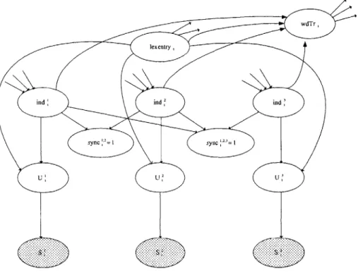
where P(sIM) is referred to as the pronunciation model and P(ols) is referred to as the acoustic model. To understand this representation in the context of the Feature-Based Pronunciation model, a general diagram of the speech application's DBN is shown in figure 9 (shaded nodes means that they are observable).
wdTr,
lexentry
ind ind ind
sync = sync 3=
U U2U
Figure 9: A Single Frame Feature-based Pronunciation Model DBN
The U/, syncj3a, ind,, lexEntry, and wdTrt, variables comprise the collection of hidden variables, s, as seen in (6). The U,' nodes represent the underlying value of feature
j.
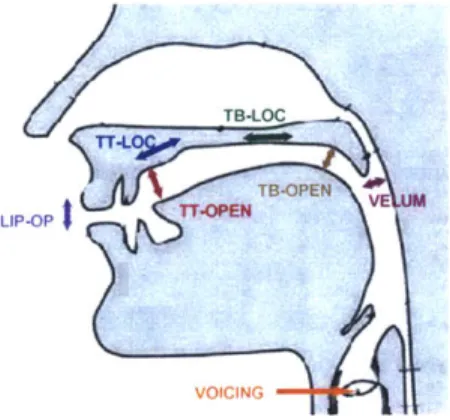
These feature values, which include the degree of lip opening, tongue tip location and opening degree, tongue body location and opening degree, velum state, and glottal or voicing state [6], essentially characterize the target word. They are shown in figure 10. The sync,;B binary variable enforces a synchrony constraint between subsets of thefeature value and is what makes this speech application unique. Most speech recognition models capture speech variations through phonemic3 substitutions, insertions, and
deletions, but the feature-based system captures them through asynchrony and changes in 3' Phonemes are the smallest units of a words. For example, the word "everybody," can be phonemically transcribed to [eh v r iy bcl b ali dx iy].
feature values. The latter three variables, ind/, lexEntryt, and wdTrt,, are used to index into various elements of the speech transcription. The lexEntry, node indexes into the current word in the 3278 word lexicon or dictionary. The ind/ node indexes feature
j
into the underlying pronunciation. The wdTr, binary variable indicates whether the current word has completed its transcription.TB-LOC,
UIP-OP TTONTB-OPEN V
VOICING
Figure 10: Phonetic Feature Values (by Karen Livescu)
The S nodes represent the observed surface value, o, seen in (5) and (6), of feature
j.
These values can stray from the underlying pronunciation in two ways: substitution, in which a feature fails to reach its target value; and asynchrony, in which different features proceed through their sequences of indices at different rates.The transcription of the word "everybody" is used in this project since it shows interesting results and has already been used extensively in previous research. Although the structure of the Bayesian network (i.e., the nodes, dependencies, and conditional probability tables) stays the same for all word transcriptions, which are taken every 10 ms, the observation values and number of frames changes from word to word. In order to make the data size more manageable for this project, the lexicon (or dictionary) is
reduced from 3278 word entries to a single word entry - the word everybody. This means that only the baseforms for everybody is used. The transcription is comprised of 16
frames, in which each frame represents a time slice of 10 ms. The frames come in three distinct forms: a beginning, middle, and end, which are needed to reflect the time transition. The three forms are shown in Appendix A. Essentially the 16 frames used in "everybody" are comprised of a beginning frame, 14 middle frames, and an end frame.
4.
Parallel System Analysis
Although most microprocessors developed are general-purpose and try to accommodate a variety of applications, it is inevitable that certain applications run better on certain
machines. This is a result of characteristics of the application, such as the inherent amount of parallelism in the algorithm, the size of the problem, and the communication pattern of the program. With this in mind, the following section defines metrics to be used in evaluating the parallel system.
4.1 Performance Metrics
Overhead Time
Overhead time is defined as the total time spent solving a problem by all the processors (pTp) over and above that required by a single processing element (T):
Speedup
Speedup measures the relative benefit of solving a problem in parallel versus solving it in series, and is defined as the ratio of the time taken to solve a problem on a single
processing element to the time required to solve the same problem on a parallel computer with p identical processing elements:
S =S (8)
TP
Speedup can never exceed the number of processing elements, p. If the best sequential algorithm takes T, units of time to solve a given problem on a single processing element, then a speedup of p can be obtained on p processing elements if none of the processing elements spends more than time Ts/p. A speedup greater than p is possible if each processing element spends less than time Ts/p solving the problem. This phenomenon is known as superlinear speedup and may occur when hardware features put serial
implementation at a disadvantage (i.e., data for a problem that might be too large to fit into the cache of a single processing element).
Efficiency
In most cases, parallel systems do not achieve full speedups. Processing elements cannot devote 100% of their time to the computations of the algorithm. Efficiency, therefore, is used to determine the fraction of time for which a processing element is usefully
E (9)
p
In an ideal parallel system, speedup is equal to p and efficiency is equal to one. In practice, speedup is less than p and efficiency is between zero and one.
Scalability
A parallel system is considered scalable if it has the ability to maintain efficiency at a fixed value by simultaneously increasing the number of processing elements and the size of the problem. This metric measures a parallel system's ability to utilize increasing processing resources effectively.
4.2 Sources of Overhead
Using twice the number of computing resources, one would think that the amount of time to complete a given task would double. However, this is rarely the case. Aside from performing essential computation, parallel programs may also be spending time in
interprocess communication, idling, and excess computation (computation not performed by the serial formulation) [7]. The following factors that contribute to overhead help describe the performance of parallel systems.
Interprocess Communication
Interprocess communication is the time spent transmitting data between processing elements and is usually the most significant source of overhead. This factor depends on the size of the problem and of the processing overhead.
Idling
Idling is caused by load imbalances, in which different workloads are distributed among different processors; synchronization, in which processing elements are waiting for one another to reach the same point in the program; and the presence of serial components in a program, which is the unparallelizable parts of an algorithm that has to run its course on a single processor as the other processors wait.
Excess Computation
Excess computation is a side effect of converting sequential algorithms to parallel algorithms. The fastest known sequential algorithm for a problem may be difficult or impossible to parallelize, forcing the use of a poorer, but more easily parallelizable sequential algorithm. Also, the different aggregate nature of serial and parallel algorithms may cause computations that were not in the serial version to be redone.
5.
Implementation of Application
5.1 Algorithm
The particle filtering algorithm, described in pseudocode in figure 7, is used to make inferences on a Bayesian network. The first stage of the algorithm is to produce many instances of the Bayesian network, called particles. Each instance of the Bayesian network is distinct since a random number generator chooses a state for each node in a particle (refer to line 6 of figure 7). Because any given node has dependencies on its parents, the state of the parent particles must be known by that node in order to determine
its own particle state. This is where most communication occurs from node to node. Next, as seen in lines 9 and 10 of figure 7, the inference is made by counting and weighting occurrences of the probabilistic event being inferred. Finally, an average of that value is taken to produce the result.
1. int main() Outer Loop:
2. for (sampleInd = 0; sampleInd < sampleNum; sampleInd++)
{
Array stores instances of the Bayesian network.
3. float particle**;
Receive values from other tiles if parents values are needed. 4. parentState =static receive(); Inner Loop:
5. for (rvInd = 0; rvInd < n; rvInd++)
{
Select state of random variable using random number generator and parent state values.
6. state = fn (parentState, random number);
Store state of random variable in particle array.
7. particle[sampleInd] [rvind] = state;
}
Send values to other tiles if for all random variables that have child nodes in another tile.
8. staticsend(state);
}
Count up samples and divide by weight (refer to particle filtering algorithm example in Section
3.1).
9. count = fn(particle[sampleInd) [rvInd],evidence);
10. ans = count/weight;
11. return(ans);
Figure 7: Pseudocode describing the Particle Filtering Algorithm
The algorithm is comprised of two main loops: an inner loop (refer to line 5 of figure 7), which cycles through each Bayesian network variable, and an outer loop (refer to line 2 of figure 7), which cycles through each sample. The mapping procedure involves
decreasing the size of these loops by distributing them among the tiles. A coarse grain mapping would correlate to splitting up the outer loop, which distributes the number of
sampling loops among the tiles. A medium and fine grain mapping would correlate to splitting up the inner loop, which distributes the random variables of the Bayes network among the tiles. Note that data is sent at the end of each outer loop and received at the beginning of this loop. Therefore, once a tile sends its values to all dependent tiles and
receives all values from a parent tile, it can immediately begin a new set of computation. The complete code used in this implementation can be observed in Appendix C.
5.2 Mapping
There are infinite ways to map the particle filtering algorithm on Raw. For this project, a coarse, medium, and fine grain parallelization of the algorithm are implemented. The different mappings reflect three major ways in which the sampling algorithm can be split among the tiles - by number of samples, frames, and sections of a frame per tile. These mappings should be adequate in examining the performance of the application on Raw since they cover a comprehensive range of communication patterns. Since the
communication patterns are fixed, all implementations are done using the static network on Raw. The three implementations are described below.
Coarse Grain
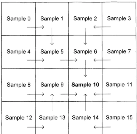
The coarse grain implementation, depicted in figure 11, parallelizes the samples taken during an inference.
Figure 11: Coarse Grain Implementation
The Bayes network and inference algorithm are independently stored and run on each tile's memory and external DRAM, but with a fraction [1/(number of tiles used)] of the total samples. For example, if the total number of sample values is 1600. In a 16-tiled Raw processor, each tile would only have to run 100 samples. Communication among the tiles is minimal for this implementation. The count value is sent from tile to tile after each
outer loop completion. Arrows in the diagram reflect the direction flow of this variable, which is pipelined and summed over all tiles only at the very end of the computation (the
final result is stored in the bolded tile).
Sample 0 Sample 1 Sample 2 Sample 3
I
Sample 4 Sample 5 Sample 6 Sample 7
Sample 8 Sample 9 Sample 10 Sample 11
Medium Grain
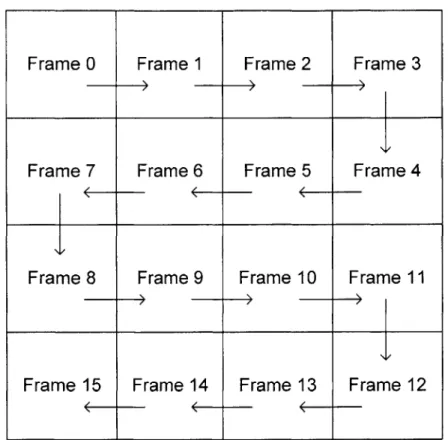
The medium grain implementation, depicted in figure 12, parallelizes the evaluation of frames in an inference.
Figure 12: Medium Grain Implementation
The total number of frames in the Bayesian network is distributed among each tile. Since each frame has approximately the same number of nodes (~40), the loads are well-balanced if the same number of frames is mapped onto each tile. In this implementation,
16 frames are used. Therefore, one frame is mapped onto each tile. Nodes on any given frame (besides the first and last one) have dependencies on parent nodes in the frame directly preceding it. The arrows in the diagram reflect the direction of data flow and,
Frame 0 Frame 1 Frame 2 Frame 3
Frame 7 Frame 6 Frame 5 Frame 4
Frame8 Frame9 Frame 10 Frame 11
therefore, data dependencies. Exactly 18 words, which are the parent state values, are sent from frame to frame at the end of each outer loop of the program.
Fine Grain
The fine grain implementation, shown in figure 13, parallelizes the evaluation of nodes in the Bayesian network during an inference.
Figure 13: Fine Grain Implementation
In this parallelization, the frames are split up into smaller sections and each tile evaluates a fraction of the total number of nodes in a Bayesian network. In this case, a single cluster of nodes can have many dependencies; therefore, there is a great deal of
Section 0 Section 1 Section 2 Section 3
Section 4 Section 5 Section 6 Section 7
Section 8 Section 9 Section 10 Section 11
I / I I
communication among the tiles. Again, the arrows in the diagram reflect the direction of data flow (between 16 to 80 words are sent from tile to tile at the beginning of each outer loop).
In the speech recognition application, there are approximately 600 nodes; thus, for a 16-tiled implementation, approximately 38 nodes will be placed on each tile. A rough attempt to load balance4 the tiles is made. Higher priority is given to maintaining similar communication patterns among the tiles as this will effect performance more drastically. Essentially, two major communication patterns exist (refer to Appendix B): one in which data is communicated laterally along the directed acyclic graph (DAG) and the other in which data is communicated longitudinally along the DAG. Lateral communication is avoided since it hinders parallel computation. For example, in the 16-tiled fine grain parallelization, depicted in figure 13, this lateral communication is unavoidable along Section 4-7. After Sections 0-3 finish their computation, Sections 4-7 can not
immediately begin work. Sections 5-7 must idle until Section 4 completes computing and sends its values to Section 5. Similarly, Sections 6-7 are idle until Section 5 completes its work. This domino pattern continues until Section 6 finishes computation. Without this
section of the implementation, there would be less idle time.
4 In load balancing, several factors were recognized as contributing to more work. These factors include the number of nodes placed in each partition and the size of the conditional probability of the nodes (bigger tables have greater memory latency).
6.
Results
The coarse, medium, and fine grain implementations are evaluated using the metrics described in Section 4. The results are described below. (If not noted, all results are taken with the number of samples, N, taken set to 100.)
Overhead
A plot of the overhead for all three implementations is shown in figure 14. At p = 2, where p is the number of processors, the overhead for the medium and fine grain implementations spike up. This is because instructions have to be stored in the external DRAM of Raw5, resulting to more cache misses and longer memory latencies then when
more processors are used. Since instruction memory is able to fit onto each tile for p > 2, it may be best to observe a trend at p = 4.
5 The instruction memory for a single Bayesian network and inference algorithm is approximately 7.4
megabytes. Since each tile can store only 32 kB of instruction memory, the remainder is placed in the external DRAM and is cached in the tiled processor when used.
x 14 8 Overhead
2. a a a
-fp-esosinraes h Coarse Grain
Medium Grain Fine Grain
0 12 4 8 1
Number of Processors
Figure 14: Overhead
Beginning at p 4, the overhead for the coarse and medium grain
implementations increase, but decreases for the fine grain implementation as the number of processors increases. The coarse grain implementation overhead increases because the
Bayes net and inference algorithm are replicated on each tile; therefore, each tile has to load up the same set of data. An increase in the number of processors would obviously result to an increase in the total load up time for all processors. Also, instructions on each tile are stored in DRAM; therefore, increasing the frequency of cache misses and
increasing memory latency. For the medium grain implementation, the problem size is split among the tiles (not replicated), so the total load-up time should remain about the same as the number of processors increase. The cause for the increase in overhead is its
increase in idle time. Although the medium grain implementation reaches a point at which all tiles are doing work, the start up period (or time it takes to saturate all compute processors) is costly. Because of data dependencies, many tiles have to wait for values to
propagate. For example, if 16 processors are used for the medium grain implementation not all 16 tiles can start computation at once. The first tile to begin computation would be the one containing frame 1. After that tile completes its computation, it sends its values off to the tile containing frame 2, and so forth. The fine grain implementation is the only one that shows a decrease in overhead because, similar to the medium grain
implementation, the problem size is split up among the tiles and does not add to the total load up time and, similar to the coarse grain implementation, more then one tile can begin computation at once at startup. For the 16-tile implementation, for example, four tiles (section 0-3 of figure 13) can begin running simultaneously since those tiles are not dependent on each other. The next four tiles (Sections 4-7 of figure 13) can run in parallel next. At that stage, however, there are some interdependencies among the tiles (shown by the arrows), which result to some idle time. The remaining 8 tiles proceed the same way as the beginning sets. Therefore, full computation power can be achieved more quickly than in the case of the medium grain implementation.
Speedup
Speedups for all implementations increase. The coarse and medium grain graphs follow closely together with the medium grain dipping slightly below the coarse grain, whereas the fine grain ramps up considerably as the number of processors increases. This trend is seen in figure 15.
Speedup 5 ---- --- - -- - --- --- -- Coarse Grain -- Medium Grain --Fine Grain 0 0 2 4 6 10 12 14 16 Number of Processors Figure 15: Speedup
The coarse grain implementation achieves almost maximum linear speedup
because each tile is doing work at all time. Also, the coarse grain implementation does not require much tile-to-tile communication. The medium grain implementation starts to dip below the coarse grain implementation at p = 4 because of the overhead. At p = 4, the fine grain parallelization exhibits superlinear speedup. It surpasses both the coarse and medium grain parallelization significantly because, as discussed in the previous section, its overhead decreases as the number of processors increase.
Efficiency
The coarse grain efficiency follows one as seen in the efficiency plot in figure 16. This is true because all tiles are doing work most of the time and no tiles are idling. The medium grain implementation starts to dip after p = 4 because of overhead, which causes many
superlinear phenomenon described earlier. At p = 2, there is a dip in efficiency because there is a spike in overhead at that point caused by increased cache misses and memory latency. 1.2 --- --- +- L--- ---, ---.1 ---+ --- -- --+ --- -+ - --- +---0.6 ---- - -- --- --- --- -- M eLr r i 1.2 0.5 2 4 6 8 10 12 14 16 Number of Processors Figure 16: Efficiency Scalability
As a reminder, scalability is the trend of efficiency as the problem size and number of processors increase. Each entry in tables 1-2 is an efficiency value. The number of samples is set at 10, 100, and 1000.
Efficiency for the coarse grain implementation is close to I at all times for all three sample number values; this implementation is therefore considered scalable. Scalability results for the medium grain implementation are shown in table 1.
p=1 p= 2
1 0.830971
1 0.904433
1 0.807354
Table 1: Scalability Results
p =,4 p = 8 p
0.834299 0.635772 0.
1.038937 1.005005 0.
0.943254 0.944778 0.
for Medium Grain Implementation
For problem sizes greater than 100, the medium grain implementation becomes less scalable. One would expect the opposite result since a greater sampling number would compensate the cost of the startup overhead. However, memory once again hinders performance. The particle array, seen in the pseudocode of figure 7, stores all samples taken before taking a tally and weighted average. Therefore, at n = 1000, the array becomes so big6 that data begins to spill into DRAM. This would cause an increase in
cache misses and memory latency, leading to a decrease in system efficiency.
p=l p=2
1 0.569623
1 0.587097
1 0.520544
Table 2: Scalability Results
p=4
0.859399
1.078245
0.961245
for Fine Grain
p=8 p=16
1.130776 1.265892
1.165623 1.270941
1.03848 1.188685 Implementation
Similarly, table 2 shows the fine grain implementation become slightly less scalable as n increases. This is caused by the same data memory problem as the medium grain
implementation.
6 A particle array is an NxM array of integers (4 bytes), in which N is the number of samples and M is the
number of random variables on each tile. For N = 1000, the particle array for the medium and fine grain
implementations, which have approximately 40 random variables per tile, is 4 bytes * 40 * 1000 = 160 kB.
The total first level data memory on Raw is only 32 kB. Therefore, memory overflow occurs when N =
200. n=10 n = 100 n = 1000 = 16 435403 943838 728979 n= 10 n = 100 n = 1000
The coarse grain implementation does not show the same decrease in scalability because the samples are parallelized among the tiles. For bigger problem sizes (around n
= 1200), the coarse grain implementation will most likely encounter data memory overflow.
7.
Conclusion
All implementations have good results only within certain parameter limits. The coarse grain implementation achieves maximum linear speedup and is efficient and scalable only if the problem size is restricted to about 1000 samples. Any problem size greater than that value will result to a decrease in performance. The medium grain
implementation shows poor results. It achieves linear speedup and efficiency up to only p
= 4. After that point, the heavy startup overhead starts to affect its performance, resulting
to a decrease in speedup and efficiency. Scalability also decreases as the problem size increases for the medium grain implementation. This is found to be the result of data memory overflow to the DRAM. The fine grain implementation surpasses the coarse grain results for speedup and efficiency within the limits of 1000 samples because for p > 2, instructions do not have to be dumped into DRAM. In the scalability results, however, the efficiency of the fine grain implementation begins to drop like the medium grain
implementation. This is a result of data memory overflow as well.
A major problem with Raw is that it is unable to accommodate all instructions and data of the speech application on local memory all the time. When the problem size gets too big, the instructions or data have to be dumped into the external Raw DRAM. This causes a decrease in performance as the system experiences greater cache misses and
memory latency. Also, in the coarse grain implementation, the instruction memory is so big that it also has to be placed in external memory. Better speedup and efficiency can be attained if all instructions can be stored locally on each tile.
Software solutions, however, can greatly improve the performance of Raw by reducing the amount of needed data memory. For example, the particle array can be
eliminated by having counters keep track of the tally and weight variables. This would reduce the amount of needed memory storage, thus drastically improving the
performance of the medium and fine grain implementations. It would be difficult, however, to reduce the instruction size in the coarse grain implementation so that it can fit locally onto a tile because the instruction set for the application is inherently big. Therefore, the best way to avoid this problem is by splitting up the instructions among the tiles, which is done in the medium and fine grain implementations.
Since smaller problems using the fine grain parallelization give better
performance results, as seen in the Results section, the key idea underlying the use of Raw and the speech recognition application is that the best system performance can be achieved if the least amount of data and instruction memory are used. This can be done by writing more efficient software implementations that use up less data memory and
smarter mapping procedures that can break down the instruction size of the application across the tiles.