Publisher’s version / Version de l'éditeur: Robotica, 29, January 1, pp. 59-71, 2011-01-14
READ THESE TERMS AND CONDITIONS CAREFULLY BEFORE USING THIS WEBSITE. https://nrc-publications.canada.ca/eng/copyright
Vous avez des questions? Nous pouvons vous aider. Pour communiquer directement avec un auteur, consultez la première page de la revue dans laquelle son article a été publié afin de trouver ses coordonnées. Si vous n’arrivez pas à les repérer, communiquez avec nous à [email protected].
Questions? Contact the NRC Publications Archive team at
[email protected]. If you wish to email the authors directly, please see the first page of the publication for their contact information.
NRC Publications Archive
Archives des publications du CNRC
This publication could be one of several versions: author’s original, accepted manuscript or the publisher’s version. / La version de cette publication peut être l’une des suivantes : la version prépublication de l’auteur, la version acceptée du manuscrit ou la version de l’éditeur.
For the publisher’s version, please access the DOI link below./ Pour consulter la version de l’éditeur, utilisez le lien DOI ci-dessous.
https://doi.org/10.1017/S026357471000072X
Access and use of this website and the material on it are subject to the Terms and Conditions set forth at
Efficient Constant-Velocity Reconfiguration of Crystalline Robots
Aloupis, Greg; Collette, Sébastien; Damian, Mirela; Demaine, Erik D.; Robin,
Flatland; Langerman, Stefan; O'Rourke, Joseph; Pinciu, Val; Ramaswami,
Suneeta; Sacristán, Vera; Wuhrer, Stefanie
https://publications-cnrc.canada.ca/fra/droits
L’accès à ce site Web et l’utilisation de son contenu sont assujettis aux conditions présentées dans le site LISEZ CES CONDITIONS ATTENTIVEMENT AVANT D’UTILISER CE SITE WEB.
NRC Publications Record / Notice d'Archives des publications de CNRC: https://nrc-publications.canada.ca/eng/view/object/?id=a78fd73b-5de6-4a8d-b5b5-4b4b7c11ab31 https://publications-cnrc.canada.ca/fra/voir/objet/?id=a78fd73b-5de6-4a8d-b5b5-4b4b7c11ab31
Efficient Constant-Velocity Reconfiguration of
Crystalline Robots
∗Greg Aloupis † S´ebastien Collette‡ Mirela Damian §
Erik D. Demaine ¶ Robin Flatlandk Stefan Langerman ∗∗ Joseph O’Rourke †† Val Pinciu ‡‡ Suneeta Ramaswami §§
Vera Sacrist´an ¶¶ Stefanie Wuhrer kk
August 24, 2010
∗A short version appeared at WAFR 2008 [Aloupis et al., 2008a], with title Realistic
Reconfiguration of Crystalline (and Telecube) Robots
†Universit´e Libre de Bruxelles, Belgique, [email protected]. Supported by the
Communaut´e fran¸caise de Belgique - ARC.
‡Charg´e de Recherches du FRS-FNRS. Universit´e Libre de Bruxelles, Belgique,
§Villanova University, Villanova, USA, [email protected].
¶Massachusetts Institute of Technology, Cambridge, USA, [email protected].
Par-tially supported by NSF CAREER award CCF-0347776, DOE grant DE-FG02-04ER25647, and AFOSR grant FA9550-07-1-0538.
kSiena College, Loudonville, N.Y., USA, [email protected]
∗∗Maˆıtre de Recherches du FRS-FNRS. Universit´e Libre de Bruxelles, Belgique,
††Smith College, Northampton, USA, [email protected].
‡‡Southern Connecticut State University, USA, [email protected]
§§Rutgers University, Camden, USA, [email protected]. Partially
sup-ported by NSF grant CCR-0204293.
¶¶Universitat Polit`ecnica de Catalunya, Barcelona, Spain, [email protected] .
Partially supported by projects MCI MTM2009-07242 and Gen. Cat. DGR 2009SGR1040.
Abstract:
In this paper we propose novel algorithms for reconfiguring modu-lar robots that are composed of n atoms. Each atom has the shape of a unit cube and can expand/contract each face by half a unit, as well as attach to or detach from faces of neighboring atoms. For universal re-configuration, atoms must be arranged in 2×2×2 modules. We respect certain physical constraints: each atom reaches at most constant ve-locity and can displace at most a constant number of other atoms. We assume that one of the atoms has access to the coordinates of atoms in the target configuration.
Our algorithms involve a total of O(n2
) atom operations, which are performed in O(n) parallel steps. This improves on previous reconfiguration algorithms, which either use O(n2
) parallel steps [Rus and Vona, 2001, Vassilvitskii et al., 2002, Butler and Rus, 2003] or do not respect the constraints men-tioned above [Aloupis et al., 2009b]. In fact, in the setting considered, our algorithms are optimal. A further advantage of our algorithms is that reconfiguration can take place within the union of the source and target configuration space, and only requires local communication.
1
Introduction
Self-reconfiguring modular robots. Robots designed with inflexible structures tend to have a unique purpose. They can be very efficient but often lack versatility, in the sense that they might not perform unexpected tasks efficiently, or might have problems adapting to new environments.
For this reason, since the late 80’s, much research has been
concentrated on the design of modular robots that can
self-reconfigure [Fukuda and Nakagawa, 1988]. Modular robots are theoretically capable of reaching any shape that has the same mass/volume (restricted to the size of their finer components, or modules). Thus they not only become capable of seemingly limitless uses, but they also have the ability to self-repair (by replacing damaged modules), and navigate through new environments.
Several new prototypes of modular robots appear each year. Develop-ers strive to solve hardware design challenges involving strength, precision, bonding, energy efficiency and flexibility of modules. An important goal is also to reduce module sizes. On the other hand, a significant problem in the field is to design efficient algorithms for self-reconfiguration.
Modular robots are often classified into distinct categories.
exam-ple of a cube lattice model. Early square and hexagonal lattice
examples, as well as 3-dimensional rectangular grid robots, are
found in [Chirikjian, 1994, Murata et al., 1994, Pamecha et al., 1996] and [Hosokawa et al., 1998, ¨Unsal et al., 2000]. Recent efforts have been made to define and characterize lattice robots [Brener et al., 2008]. Exam-ples of chain robots are Polypod and Polybot [Yim, 1994, Yim et al., 2000].
Finally, one can also find mixed (chain and lattice) models,
such as M-Tran [Yoshida et al., 2002]. Various types of self-reconfiguring robots, as well as related algorithmic issues, are surveyed in [Murata and Kurokawa, 2007, Yim et al., 2007]. In this paper we focus on the (modular) Crystalline [Rus and Vona, 2001, Butler et al., 2002] and
Telecube [Suh et al., 2002] robots, which are designed on a square lattice.
Crystalline and Telecube robots. The atoms1
of these robots are cubic in shape, and are arranged in a grid configuration. Each atom is equipped with mechanisms allowing it to extend each face out one unit and later retract it back. Furthermore, the faces can attach to or detach from faces of adjacent atoms; at all times, the atoms should form a connected unit. The default configuration for a Crystalline atom has expanded faces, while the default for a Telecube atom has contracted faces.
When groups of atoms perform the four basic atom operations (expand, contract, attach, detach) in a coordinated way, the atoms move relative to one another, resulting in a reconfiguration of the robot. Figure 1 shows an example of a reconfiguration.
Figure 1: Example of reconfiguring Crystalline atoms.
To ensure that all reconfigurations are possible, atoms must be
ar-ranged in k × k × k modules, where k ≥ 2 [Aloupis et al., 2009b,
Vassilvitskii et al., 2002]. In the 2D setting that we focus on, we assume
that modules consist of 2×2 atoms. Our algorithms can easily be extended
to 3D.
1In the literature, the term “module” is often used to describe an individual hardware
unit, and small collections of such units are referred to as meta-modules. Individual cubic components in the Crystalline model have also been named atoms by their designers. We will avoid using the term meta-module entirely. Instead we will call individual cubic components atoms, and larger groups will be referred to as modules.
We refer the reader to [Rus and Vona, 2001, Vassilvitskii et al., 2002, Aloupis et al., 2009b] for a more detailed introduction to these robots. The model. The problem we solve is to reconfigure a given connected source configuration of n modules to a specified, arbitrary, connected target configuration T in O(n) parallel steps. We allow modules to exert only a con-stant amount of force, independent of n. In particular, each module has the ability to push/pull one other module by a unit distance (the length of one module) within a unit of time. Simply bounding the force may still lead to arbitrarily high velocities and thus rather unrealistic motions. On the other hand, in some situations where maximal control is desired (e.g., treacherous conditions, dynamic obstacle environment, minimally stable static configu-ration of the robot itself) it may be desirable to strictly limit velocity. Thus we also bound maximum velocity (and so the momentum) by a constant (module length / unit time). One important advantage of our algorithm is that we can rely on local communication between atoms. That is, atoms can decide to move based only on the state of neighbors and instructions received from them.
Our model permits separating algorithmic issues from design consider-ations, at the same time as retaining the fundamental physical constraints of velocity and force. We assume that if a module decides to move a short distance and dock with another module, it will do so accurately and within a specific allowed time. Our algorithms are susceptible to such issues as motion uncertainties and errors, since we perform many parallel operations. It may be possible to limit such errors by only allowing a constant number of simultaneous operations, or only allowing motions along the perimeter of the robot. Such approaches have been used before, but at the cost of increased time complexity. Our approach takes advantage of the Crystalline model which permits traveling through the interior of the robot, something which has been done in many previous reconfiguration algorithms (see next section).
Under the constant-velocity model, there exist configurations which re-quire a quadratic number of overall basic moves to reach their goal. To attain the linear bound proved in this paper, one must rely on (more physically unstable) massively parallel algorithms. Having said this, we note that any instability that an atom may have (for instance, a docking delay) remains a local problem in our algorithms: moving components are isolated into small individual groups, each traveling on a fixed substrate frame. A mechani-cal problem may create a bottleneck, or “traffic jam”, but this should only affect the time-complexity, not the mechanical difficulty of recovering. In
other words, a problem encountered by one module should not cause any problems to another module.
Our algorithms rely on “parallel tunneling”, which has been used in the
PacMan algorithm [Butler et al., 2001, Butler and Rus, 2003]. The Pac-Man designers showed a tunneling experiment and discussed the troubles
encountered in such physical experiments, such as misalignments that may cause problems for atom connections. In order to improve this issue, a new Crystal connector was proposed [Butler et al., 2002], allowing a significant amount of lateral and vertical misalignment.
Our algorithms are designed for Crystalline robots. Many other modules have been and continue to be designed for reconfigurable robots. Wikipedia lists 34 modules designed as of 2010.2 Some of these modules are equivalent to Crystalline modules from the point of view of our model, and some are not. We make no attempt at a comprehensive survey. In Section 5 we discuss how our algorithms can be adjusted to work for one closely related model, Telecube robots. In that section we also mention how our algorithm can be altered to apply to robots made of other types of modules.
Related results. The optimal number of moves between
configura-tions has been studied, in the context of centralized reconfiguration
plan-ning (see [Chiang and Chirikjian, 2001, Pamecha et al., 1997]).
Central-ized reconfiguration algorithms have been proposed for many systems (e.g. see [Kotay and Rus, 2000, Yoshida et al., 2002]). Distributed algorithms to reconfigure certain classes of hexagonal modular robot configurations are given in [Walter et al., 2002]. Typically such algorithms employ heuristics or work for particular classes of target shapes. Of particular interest are distributed algorithms in which each module actuates based on local in-formation received from immediate neighbors (e.g. see [Salemi et al., 2003, Butler et al., 2004, Stoy, 2006, Kurokawa et al., 2008]).
Algorithms for reconfiguring Crystalline and Telecube robots
in O(n2
) parallel steps have been given in [Rus and Vona, 2001, Vassilvitskii et al., 2002, Butler and Rus, 2003, Butler et al., 2001]. The quadratic bound is also implied in [Chirikjian et al., 1996], which deals with reconfigurations of a specific class of modular robots (more restrictive than Crystalline). An algorithm that uses O(n) parallel steps for reconfiguring a robot within the bounding box of source and target configurations was
given in [Aloupis et al., 2009b]. The total number of individual moves
is also linear. However, no restrictions were made concerning physical
properties of the robots. For example, Θ(n) strength is required, since modules can carry tall towers and push large masses during certain operations. An O(log n) parallel step algorithm for 2D robots that uses a total of O(n log n) atom moves and also stays within the bounding box is given in [Aloupis et al., 2008b], and this has recently been extended to 3D [Aloupis et al., 2009c]. However, in this algorithm, not only are modules assumed to have Θ(n) physical strength, but they can also reach Θ(n) velocity. An O(√n) time algorithm for 2D robots, using the third dimension as an intermediate, is given in [Reif and Slee, 2007]. This is optimal in the model considered, which permits linear velocities, but only constant acceleration. If applied within the model used in [Aloupis et al., 2008b], this algorithm would run in constant time. We remind the reader that, unlike [Reif and Slee, 2007, Aloupis et al., 2009b, Aloupis et al., 2008b], we limit force and velocity to a constant level.
Contributions of this paper. We present two algorithms to reconfigure Crystalline robots in O(n) time steps, using O(n) parallel moves per time step. Our first algorithm (Section 3) is slightly simpler to describe. It also forms the basis of our second algorithm (Section 4), which is exactly in-place, i.e., it uses only the cells of the union of the source and target configurations. This is particularly interesting if there are obstacles in the environment. Both algorithms consider the given robot as a spanning tree, and push leaves towards the root with “parallel tunneling”. This form of tunneling has been used in the PacMan algorithm [Butler et al., 2001, Butler and Rus, 2003], which also works in-place but does not guarantee linear time complexity. In our algorithm, no global communication is required. This means that constant-size memory suffices for each non-root module, which can decide how to move at each step based solely on the states of its neighbors. In the realistic model considered in this paper, our algorithms are worst-case
opti-mal: transforming a horizontal row of modules to a vertical row requires a
linear number of parallel moves and a quadratic number of total operations. Our first algorithm can be adapted for use with Telecube modules. However an adaptation of our in-place algorithm seems to require more memory for non-root modules. This is discussed in Section 5. Our results are not accom-panied by simulations or experiments, but from the viewpoint of mechanics and electronics, we are only requiring atoms to perform basic operations sim-ilar to what appears in the experiments reported in [Butler and Rus, 2003].
2
Primitive operations
We restrict our descriptions to a 2D lattice whose cell size equals the size of one robot module (i.e., 2×2 connected atoms in their expanded state). None of our techniques depend on dimension, so it is straightforward to extend to 3D robots. Given the 2×2 module size, a cell of the lattice can potentially contain two compressed modules (see Fig. 2b). Cells can be marked with an integer in {0, 1, 2}: a 0-cell corresponds to a node in T that has no module yet, a 1-cell contains one module, and a 2-cell contains two (compressed) modules. In a 2-cell, we sometimes distinguish between the host module and the guest module: the host module is the one occupying the 1-cell prior to becoming a 2-cell; the guest module is the one compressing itself into the 1-cell occupied by the host module, thus turning the cell into a 2-cell (see Fig. 2a).
Let r0 be a specialized module that has access to a map of the target
configuration, T . We compute a spanning tree S of the source configuration,
rooted at r0, and instruct modules to form attachments corresponding to
tree edges in S. The spanning tree can be computed in linear time and constructed via local communication. The tree structure between cells is maintained throughout the algorithm by physical connections between host modules; note that guest modules are irrelevant in determining S. These modules are also responsible for the parent-child pointer structure of the tree. For each node u∈ S, let P (u) denote the parent of u in S (recall that both u and P (u) are host – not guest – modules). A child of a cell u is adjacent either on the east, north, west, or south side of u. Let the highest
priority child of u be the first child in counterclockwise order starting with
the east direction.
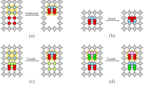
Let m and q be adjacent cells. We define the following primitive operations (illustrated in Fig. 2). A cell is meant to be engaged in at most one operation at any time.
1. PushInLeaf(m, q) – applies when q = P (m), m is a leaf, and both are uncompressed. Here, m becomes empty and q becomes compressed (i.e., q takes the module of m as a guest).
2. PopOutLeaf(m, q) – applies when q is compressed and m is empty. This is the inverse of the PushInLeaf operation.
3. Transfer(m, q) – applies when m is compressed and q is non-empty; if q is compressed, the guests of both cells physically exchange posi-tions. Otherwise, the guest of m moves into (and becomes a guest of)
q.
4. Attach(m, q) – applies when the host modules in m and q are unattached. The two modules make a physical connection.
5. Detach(m, q) – applies when the host modules in m and q are at-tached. The two modules break their physical connection.
6. Switch(m) – applies when m is compressed. Its two modules physi-cally switch positions (and roles of host and guest).
PushInLeaf
Switch
(a) (b)
Transfer Transfer
(c) (d)
Figure 2: (a) PushInLeaf. Cell q has a shaded background. In PopOut-Leaf which is the inverse of this diagram, q would be the empty cell. (b) Switch: guest and host exchange their roles and positions. (c) Transfer, when only one module is compressed. Cell q is shaded. (d) Transfer, when both modules are compressed. Only initial and final configurations are shown. Note that neighboring cells are not completely drawn.
In the remainder of this paper, we assume that all parallel motions are synchronized. However, due to the simple hierarchical tree structure of our robots, we find it plausible that our algorithms could be implemented so that modules may operate asynchronously.
Lemma 1. Operations PushInLeaf, PopOutLeaf, Switch and Trans-fer maintain the tree structure of a robot and can be executed in O(1) time.
Proof. When each of the first three operations is performed individually, the
of host module q temporarily displace, in order to let those of m occupy intermediate spaces. However, at all times one of the two atoms along every face of q (other than the one adjacent to m) will remain in its original position so that connectivity is ensured; this property can be verified in Fig. 7 in the appendix. Note that the activity within guest module m does not affect connectivity in the rest of the robot.
This temporary displacement can cause connectivity issues if modules neighboring the host module q are also performing basic operations. To avoid any problems, we can subdivide one basic time unit into four subunits, so that each host module acts when it has the right parity of row and column. For example, in the first time subunit, modules located in (odd row, odd column) lattice cells are allowed to reconfigure; in the second time unit, (odd row, even column) modules reconfigure; and so on.
This way, when a leaf pushes into its parent, we can ensure that no other cells adjacent to the parent are active. This issue is even simpler to resolve in 3D, where the actuation at the atomic level can be done by 2D layers.
Now consider the Transfer operation. In this operation, two adjacent cells interact and it is best not to let any of the six neighboring cells perform basic operations simultaneously. A similar lattice parity solution can be applied.
Regarding the tree structure, it is straightforward to see that Switch and Transfer only affect module positions, while PushInLeaf removes one leaf module from S and PopOutLeaf adds one leaf module to S.
As for the complexity of the primitive operation, note that any permu-tation of atoms within a lattice cell containing two modules can be realized in linear time with respect to the size of the module (i.e., O(1) time for our modules). Thus a compressed cell may transfer or push one module to any direction, and two modules within a cell can switch roles in O(1) time.
In our basic motions, modules move by one unit length per time step. The two modules involved in a primitive operation do not carry other mod-ules. Thus our reconfiguration algorithms place no additional force con-straints beyond those required by any reconfiguration algorithm.
2.1 Details of the primitive operations
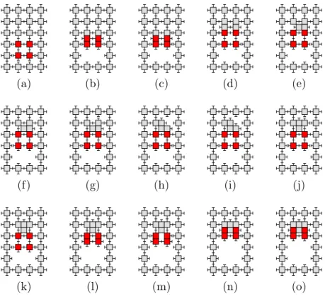
Refer to Figures 7-11, located in the Appendix. Fig. 7 shows the finite sequence of basic atom operations (attach, detach, compress, expand) that implement PushInLeaf and PopOutLeaf, which are inverse operations.
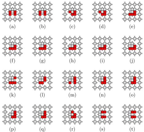
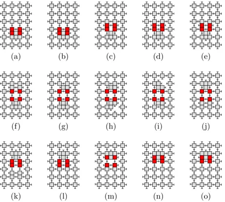
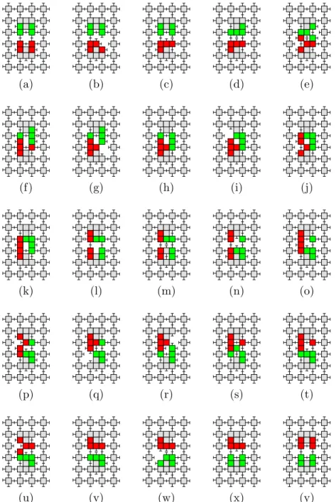
Transfer(m, q) can be described as a two-step operation. In the first step, module m is rotated within its lattice cell, in order to face module q. We call this the positioning step. In the second step, the module m is actually sent to the lattice cell of q. Depending on whether q was compressed or uncompressed, we call this the send or the exchange step. Fig. 8 shows the finite sequence of basic atom operations (attach, detach, compress, expand) that produce the positioning step. Fig. 9 and Fig. 10 show the analogous sequence for the send and the exchange steps. Transfer is the result of appropriately concatenating these steps.
Switch is a particular permutation of atoms within a lattice cell con-taining two modules, which can be realized in linear time with respect to the size of the module. Fig. 11 shows the details of the Switch operation.
3
Reconfiguration via canonical form
This section describes an algorithm to reconfigure S into T via an interme-diate canonical configuration. Modules follow a path directly to the root r0, and into a canonical “storage configuration”. We focus on the construction of one type of canonical form, a vertical line V . In fact V could be any path that avoids the source configuration. Thus the entire reconfiguration can take place relatively close to the bounding box of S. Reconfiguring from V to T is nearly the inverse procedure and is relatively straightforward. Each module m passes from the canonical form through r0. It suffices for r0 to provide m with just a few bits of information, indicating where m should have children. If we can afford to let m store O(log n) bits, then we can even specify the size of the subtrees rooted at m (this helps heuristically, and is described at the end of section 3). For this task, it is assumed that r0has ac-cess to a map of T (perhaps stored in memory, or via direct communication with some external processor).
3.1 Algorithmic details
Our algorithm reconfigures S into a vertical strip V that begins at the
maximum y-coordinate of S. We first move r0 to a maximum possible
y-coordinate: this involves pushing in a leaf and iteratively transferring it to r0, so that r0becomes part of a 2-cell and is then able to iteratively transfer to a module of maximum y-coordinate. Note that this step might not be necessary in implementations in which all modules are capable of playing the role of r0 (for example, if all modules have a map of T , or if all are capable
of communicating to an external processor). This initial step is followed by
two main phases, during which r0 does not move.
In the first phase, we repeatedly apply procedure ClusterStep to move modules closer to r0. This is done by compressing leaves into their parents, and moving up S in parallel. The shape of S shrinks during this procedure, as PushInLeaf operations in ClusterStep compress leaf modules into their parent cells. At the end of this phase, all non-leaf cells will become 2-cells. We refer to S in this state as being fully compressed. It is not critical that all cells become compressed; in fact, we can proceed to the next phase as soon as the root becomes part of a 2-cell. The restriction for S being fully compressed at the end of this phase will merely simplify our analysis of the total number of parallel steps in our algorithm.
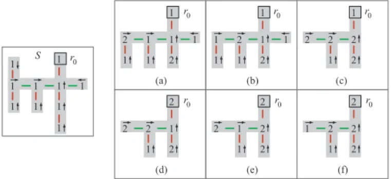
ClusterStep(S)
For all cells u in S except for that containing r0, execute the following in parallel:
If P (u) is a 1-cell
If u is the highest priority child of P (u) and all siblings of u are leaves or 2-cells,
If u is a 1-cell leaf then PushInLeaf(u, P (u)). If u is a 2-cell, then Transfer(u, P (u)).
SourceCluster(S)
Repeat until S is fully compressed ClusterStep(S).
The procedure SourceCluster is illustrated in Figure 3. The task of compressing a parent cell P (u) falls onto its highest priority child, u. Note that P (u) first becomes compressed only when all its subtrees are essentially compressed. That is, even if u is ready to supply a module to P (u), it waits until all other children are also ready. This rule could be altered, and in fact the whole process would then run slightly faster. Here, we ensure that once the root of a subtree becomes compressed, it will be able to supply a steady stream of guest modules to its ancestors.
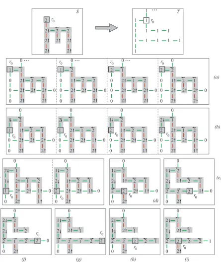
In the second phase, we construct V while emptying S, one module at a time. This is described in the second step of algorithm TreeToPath, and is illustrated in Figure 4.
1 1 1 1 1 1 1 1 S 1 1 1 2 1 1 2 1 1 1 1 1 1 2 2 1 1 1 2 1 2 2 2 1 2 1 2 2 1 2 2 1 1 2 2 2 1 1 2 2 2 2 (a) (b) (c) (d) (e) (f) r0 r0 r0 r0 r0 r0 r0
Figure 3: An example of SourceCluster. Arrows indicate the direction of the Transfer and PushInLeaf operations. After steps (a) through (e), the source configuration (left) becomes fully compressed (f).
Algorithm TreeToPath(S, V )
1. SourceCluster(S)
2. Let d be the cell containing r0as a host. Let V ={d}.
Repeat until V contains all modules:
a) For all 2-cells u in V , execute in parallel: Let c be the cell vertically above u. If c is empty, PopOutLeaf(u, c);
Otherwise, if c is a 1-cell, Transfer(u, c). b) ClusterStep(S)
1 1 1 1 1 1 1 2 2 2 r 2 1 1 2 2 2 1 (a) 1 1 1 2 2 1 2 1 1 1 2 2 1 1 (b) 2 1 1 1 2 2 1 (c) 1 1 2 2 1 2 1 1 1 1 2 2 1 2 2 1 (d) 1 1 2 2 1 2 1 1 2 2 1 1 1 2 (e) 2 2 1 2 1 2 1 2 2 1 2 1 (f) 1 2 2 1 2 1 2 2 1 1 1 1 1 2 (g) 2 1 2 1 2 1 2 2 1 1 1 2 1 (h) 2 2 1 2 1 2 1 1 2 2 0 r0 r0 r0 r0 r0 r0 r0 r0 r0 r0 r0 r0 r0 r0 r0 r0
Figure 4: An example of TreeToPath. For each step, the two phases (PopOutLeaf or Transfer, and ClusterStep) are shown.
Lemma 2. If S is a set of modules physically connected in a tree of cells,
then ClusterStep(S) returns a tree containing the same set of modules, while maintaining connectivity. So does SourceCluster(S).
Proof. ClusterStep invokes two basic operations, PushInLeaf and
Transfer. By Lemma 1, these operations independently maintain a tree. Since u is involved in PushInLeaf or Transfer (with P (u)) only if it is a 1-cell leaf or a 2-cell respectively, but also only when P (u) is a 1-cell, we know that P (u) is not involved in any other such operation in parallel. Therefore every cell is involved in at most one basic operation at a time. The claim also follows immediately for SourceCluster.
Define the height of a cell in S to be the longest path to a leaf in its subtree, plus 1. By convention, leaves have height one.
Lemma 3. Let r be a cell in S with height h ≥ 2. In iteration h−1 of
SourceCluster(S), r becomes a 2-cell for the first time.
Proof. Prior to the first iteration, S contains only 1-cells. The proof is by
induction on h. For the base case when h = 2, the children of r are leaves. Therefore, in the first iteration, during ClusterStep, the highest priority leaf compresses into r.
Now assume inductively that the lemma is true for all subtrees of height
smaller than h. Cell r must have at least one child c with height h−1. By
the inductive hypothesis, c becomes a 2-cell in iteration h−2, and all of r’s other non-leaf children are 2-cells by the end of iteration h−2. Therefore, at iteration h−1, for the first time the conditions are satisfied for r to receive a module from its highest priority child during ClusterStep.
Lemma 4. In iteration i of SourceCluster, let r be a 2-cell with height h that transfers its guest module to P (r). Then at the end of iteration i+1,
r is either a leaf or a 2-cell again.
Proof. First note that at the beginning of iteration i+1, r is a 1-cell and
P(r) is a 2-cell. Thus if r is a leaf after iteration i, it remains so. On the other hand if r has children (h≥ 2), it will become a 2-cell. We prove this by assuming inductively that our claim holds for all heights less than h. Consider the base case when h = 2. At the end of iteration i, all children of r are still leaves and thus one will compress into r (note that r might also become a leaf in this particular case).
For h > 2, consider the iteration j < i in which r received the guest module that it later transfers to P (r) in iteration i. At the beginning of
iteration j, all of r’s children were leaves or 2-cells, since that is a requirement for r to receive a guest. Let c be the child that passed the module to r. If c used the PushInLeaf operation, then at the end of iteration j, r has one fewer children (but at least one). The other children remain leaves or 2-cells until iteration i + 1, when r becomes a 1-cell again. Thus in iteration i+1, conditions are set for r to receive a module.
On the other hand, if c used the Transfer operation, we apply the
inductive hypothesis: at the end of iteration j+1 ≤ i, c is either a leaf
or a 2-cell. During iterations j and j+1 in which r is busy receiving or transferring a module, all other children of r (if any) remain leaves or
2-cells. Therefore in iteration j+2 ≤ i+1, the conditions are set for r to
receive a module.
Define the depth of a cell in a tree to be its distance from the root. Hence, the root has depth zero. Let the root of S be at height h0.
Lemma 5. SourceCluster terminates after at most 2h0−1 iterations of
ClusterStep.
Proof. We claim that at the completion of iteration h0−1+d of SourceCluster, all non-leaf modules at depth less than or equal to d in S are 2-cells (here we use S to refer to the current instance of the dy-namically changing tree, not the original S). The proof is by induction on d. The base case is the root of S at depth d = 0. By Lemma 3, the root becomes a 2-cell in iteration h0− 1. Assume inductively that our claim is true for all values d′, where 0≤ d′ < d.
Now consider a cell p at depth d−1 that has children. By the inductive
hypothesis, p and all its ancestors are 2-cells by the end of iteration i = h0−1+(d−1), and p is the last of this group to become a 2-cell. Thus at the beginning of iteration i, all children of p are either leaves or 2-cells. During iteration i, only p’s highest priority child c changes, either by transferring a guest module into p (if c is a 2-cell), or by pushing into p (if c is a 1-cell leaf). In the first case, by Lemma 4, c will be a 2-cell or a leaf by the end of iteration i+1. In the second case, c is not part of S anymore.
Since p will not accept new guest modules after iteration i (because all its ancestors are 2-cells), all siblings of c remain leaves or 2-cells during iteration i+1. Thus at the end of this iteration, our claim holds for depth d. By setting d = h0, our result follows.
Let a long gap consist of two adjacent 1-cells that are not leaves. A tree is root-clustered if it has no long gaps. Observe that a fully compressed tree is a special case of a root-clustered tree.
Lemma 6. Let S be a root-clustered tree. Then after one application of ClusterStep(S), S remains root-clustered.
Proof. This follows from claims in the proof of Lemma 4. Specifically,
con-sider any 2-cell u. If ClusterStep keeps u as a 2-cell, then u is not part of a long gap. Otherwise, if u sends a module to P (u), none of the children of u attempt to transfer a module to u. Now consider any 1-cell non-leaf child y of u. Since there was no long gap in S, all children of y were either 2-cells or leaves. Thus y will become a 2-cell during this iteration of ClusterStep. Again we conclude that u cannot be part of a long gap.
Theorem 1. Algorithm TreeToPath terminates in linear time.
Proof. By Lemma 5, SourceCluster terminates in linear time. In fact by
treating the final top position of V as an implicit root, our claim follows. More specifically, however, we analyze the transition from S into
V. When SourceCluster terminates, S is fully compressed (i.e.,
root-clustered), and we set r0 to be the host in cell d.
First we mention that all basic operations are performed legally, that is, every cell is involved in at most one operation. In step 2a, every 2-cell is involved in an operation, only if the cell above it is not a 2-cell. Therefore both cells are only involved in this operation. Step 2b is safe, by Lemma 2. In step 2a, d sends a module to the empty position c vertically above, if c is not a 2-cell. We may treat the position c as P (d), and consider step 2a to be synchronous to step 2b. In other words, d is the only child of c, and thus d follows the same rules as ClusterStep. In fact, since S is fully compressed, after the first iteration of phase 2, the tree rooted at c will be root-clustered (only c and the highest-priority child of d will not be 2-cells). Therefore, by Lemma 6, in every iteration of phase 2, S remains root-clustered. Thus in every even iteration, d supplies a module to c, and in every odd iteration d is given a module from one of its children. Informally, when d sends a module up into V , the gap (in the sense of lack of guest module) that is created in S travels down the highest priority path of S until it disappears at a leaf. In general, a guest module on the priority path will never be more than two steps away from d, following the analysis of Lemma 4. Within V , a stream of guest modules, two units apart, will move upward. One module will pop up into an empty cell, every three iterations. Thus compressed modules in V are always able to progress.
We now briefly discuss the reconfiguration from V to T . If we merely wish to construct the shape of T , then we can assume that V does not
intersect the cells that will be occupied by T . Otherwise, if T must occupy specific cell coordinates, it is trivial to move V to a position where our assumption will hold.
For the construction of T , let us first assume that the memory of each module suffices to count to n. All modules from V pass through the root r0 on their way to T . Once a module m reaches r0, the root determines the position of m in T and supplies m with three values corresponding to the sizes of the three subtrees of m in T . Then r0 transfers m to the
highest-priority child c of r0 whose subtree is not full yet. The child c in turn
transfers m to its own highest-priority child not yet full and so on, until m encounters the conditions to pop into an empty cell in T , as directed by its host module. From that point on, m simply awaits modules transferred by its parent and directs them to its children according to our priority rules (counterclockwise starting with the east child). In order to decide where to send an incoming module, m keeps count of all modules passed through; this information, along with the information collected from r0 (the sizes of its three subtrees), suffices for m to avoid sending an incoming module into a completed subtree.
If we do not have the luxury of allowing modules to count, we do the following. The root does not tell m the size of its subtrees, but instead it just tells m if it will have a subtree, in each direction. Priority rules are followed, as before. The only difference is that when m reaches its final position, it will not be able to determine when its subtrees are full. Thus each module performs an entire Depth-First Search of the partial structure of T . This involves backtracking, which can be dealt with via Transfer. We omit details here, since this backtracking issue appears again and is clarified in section 4.
We remind the reader that our first phase need not terminate before the second commences. By compressing leaves and sending them towards the root, while simultaneously constructing V from the root whenever it be-comes compressed, the target configuration will be constructed even faster. Splitting into two distinct phases simply helps with the analysis.
4
In-place reconfiguration
This section describes an in-place algorithm that reconfigures S into T by restricting the movement of all modules to the space occupied by S∪ T , as long as they intersect. If S and T do not intersect, then we also use the cells on the shortest path between them. Our description assumes intersection.
If all modules were to know which direction to take in each time unit (for example, by having an external source synchronously transmit instructions to each module individually), then it would not be difficult to design an in-place algorithm similar to the one in Section 3. However, since we impose the restriction that all modules are only capable of communicating locally, it is up to r0 to direct all action.
4.1 Overview
Our algorithm consists of two phases. The first phase is identical to phase 1 of the TreeToPath algorithm from Section 3 (i.e., clustering around the root).
In the second phase, r0 carries out a DFS (depth-first search) walk on
T, dynamically constructing portions that are not already in place. Apart
from modules in cells adjacent to r0 that receive its instructions, all other
modules simply try to keep up with r0 (i.e., they follow ClusterStep).
Note that if r0is not initially inside T , it first must travel to such a position. At any time, this “moving root” will either be traveling through modules that belong to the partially constructed tree T , or will be expanding T beyond the current tree structure, using compressed modules that are tagging along close to r0.
4.2 Algorithmic details
The InPlaceReconfiguration algorithm maintains a dynamically
chang-ing tree S, and a connected subset Sℓ of that tree. Each cell u maintains
two links: a physical link corresponding to the physical connection between
u and P (u) in S, and a logical link that is only present between adjacent
nodes in Sℓ. We call the tree Sℓ induced by the logical links the logical tree. Tree S always contains all occupied cells. Tree Sℓ is the smallest subtree of S that contains modules not in their final position in T . Thus at the end of the algorithm, S = T and Sℓ =∅.
Algorithm InPlaceReconfiguration(S, T )
Phase 1. S← SourceCluster(S). Phase 2. Sℓ← S.
Repeat until r0 reaches the final position in its DFS traversal:
S← TargetGrow(S, T ).
We continue with a description of the operation of TargetGrow. TargetGrow(S, T )
d← next cell in the DFS visit of T .
c← current 2-cell in which r0 is a guest module.
{1. DFS Root Update } Mechanical/Physical Operations 1.1 If d is a 0-cell, PopOutLeaf(c, d) 1.2 If d is not a 0-cell, If c6= P (d),
Attach(c, d) and Detach(d, P (d)). Transfer(c, d).
Tree Structure Update
1.3 Set P (c) to be d. Set P (d) to null. 1.4 Mark c as “visited”.
1.5 Add edge (c, d) to Sℓ.
{2. Root Clustering }
Until c and d become 2-cells, repeat:
(a) Leaf Prune: For all 1-cell leaves u∈ Sℓ, execute in parallel:
If u is marked “visited”, remove u from Sℓ.
(b) ClusterStep(Sℓ)
If r0is not the guest in c, Switch(d).
Note that in Phase 2, we start with Sℓ = S. Throughout this phase, the
structure of Sℓ is identical to the structure of S, with the exception that some branches of the tree Sℓ are logically trimmed off through iterative leaf prune operations. The host module in each cell uses a bit to determine if the cell is also part of Sℓ. Pointers between cells and their parents apply for both trees.
The main idea of the target growing phase is to move r0 through the
a steady stream of modules to fill in empty target cells that r0 encounters. The algorithm repeats the following main steps:
1. DFS Root Update: r0 is the guest of 2-cell c and is ready to depart.
It marks c as “visited” (i.e., c now belongs to T ). Then r0 moves to the next cell d encountered in a DFS walk of T . This is accomplished
either by uncompressing (popping) r0 into d (see Fig. 5(a → b)), or
by transferring r0 to d (see Fig. 5(e → f)). Cell d is added to Sℓ, if not already included.
2. Root Clustering: Modules in Sℓ attempt to move closer to r0, to
en-sure that they are readily available when r0 needs them. However,
host modules in their final target position should never be displaced from that position, so we must carefully prevent such modules from
compressing towards r0. To achieve this, we alternate between the
following two steps, until c and d both become 2-cells:
(a) Logical Leaf Pruning: remove any 1-cell leaf of Sℓ that has been visited (i.e., is in T ). Note that a pruned 1-cell may end up back in Sℓ one more time, during Root Update.
(b) Cluster Step: this step is applied to Sℓ. Thus, only modules that are guests or unvisited leaves will try to move towards r0. Fig. 5 illustrates the InPlaceReconfiguration algorithm with the help of a simple example.
4.3 Algorithm correctness and complexity
Lemma 7. Algorithm InPlaceReconfiguration maintains a physically
connected tree that contains all modules.
Proof. By Lemma 2, SourceCluster produces a tree S containing all
robot modules. Thus we must show that TargetGrow maintains such a tree when it receives one as input. We first analyze step 1 (DFS root update). In step 1.1, PopOutLeaf maintains a tree, by Lemma 1. In step 1.2, d is already part of S. Now if c6= P (d), we attach c to d, which creates a cycle. However, we immediately break this cycle by detaching d from P (d),
and thus S is restored to a tree. See Figs. 5(c → d → e) for an example.
Regardless of the initial relationship between c and P (d), and the possible re-structuring of S, we proceed with Transfer(c, d), which maintains tree connectivity, by Lemma 1.
2 2 2 1 2 2 2 2 2 0 0 0 1 0 0 ... 2 2 2 1 2 1 2 2 2 0 0 0 2 0 0 ... 2 2 2 2 2 2 2 2 2 2 2 1 2 2 2 2 2 2 0 0 0 1 0 0 ... S (a) 2 1 2 2 2 2 1 0 0 0 2 0 0 1 1 1 1 1 1 1 1 1 1 1 1 ... 1 T 2 1 2 2 2 2 1 0 0 1 1 0 0 2 2 2 2 2 2 1 2 1 1 2 0 0 1 2 0 0 2 2 2 1 2 2 2 2 1 0 0 2 1 0 0 2 1 2 2 1 2 1 1 2 0 0 2 2 0 0 2 1 2 2 1 2 1 1 2 0 1 1 2 0 0 2 1 2 1 2 2 2 1 1 0 2 2 1 0 0 2 (b) (c) (d) 2 1 2 2 2 1 1 0 2 2 1 0 0 2 (e) 2 1 2 2 2 1 1 0 2 2 1 0 0 2 1 1 2 2 2 2 0 2 2 2 0 0 2 (f) 2 2 2 1 1 2 2 1 2 1 0 0 2 (g) 2 2 1 2 1 2 1 2 1 2 0 0 2 (h) 2 2 1 2 1 2 1 2 1 2 0 0 2 (i) r0 r0 r0 r0 r0 r0 r0 r0 r0 r0 r0 r 0 r0 r0 r0 r0 r0 r0
Figure 5: Reconfiguring S into T : the top row shows S (after SourceClus-ter) and T . Links in Sℓ, which is shaded, are depicted as arrows. Subse-quent figures show S (with its logical subtree Sℓ shaded) (a) after Target-Grow, with each intermediate step illustrated (DFS root update on the left and the subsequent 3 clustering steps on the right); (b) after TargetGrow, with each intermediate step illustrated; (c) after TargetGrow, with its two main steps (root update and root clustering) illustrated; (d,e,f,g) show the next 4 TargetGrow steps; (h) after the next 2 TargetGrow steps;
(i) after the next TargetGrow (note the rightmost 1-cell leaf getting
After steps 1.1 and 1.2 or the DFS update, no other physical connections are altered. Pointers are modified to reflect the physical changes made. Since the root acts alone, our assumption that every cell is involved in one operation at a time holds.
Finally, S remains a physical tree during step 2 of TargetGrow. This basically follows from two observations: (a) step 2a changes only the logical
tree Sℓ, and (b) ClusterStep maintains a tree, by Lemma 2. The only
issue remaining is to prove that whenever a 1-cell leaf becomes involved in PushInLeaf in ClusterStep, it is not visited. Not only do we wish to avoid moving visited 1-cells, but this operation could cause a physical disconnection if S6= Sℓ. It suffices to claim that Sℓ never contains a visited 1-cell leaf. This is in accordance to our definition of Sℓ being the smallest tree containing unvisited modules. Given such a structure, the following situations can arise for a leaf u in step 2. The leaf u of Sℓ could remain unaltered, or if it is a 1-cell (meaning, not visited) it could use PushInLeaf to become the guest in a new 2-cell leaf. Finally if u is a 2-cell and becomes a 1-cell, we prune the 1-cell from Sℓ if it is visited.
In phase 1 of InPlaceReconfiguration, the SourceCluster call produces a root-clustered tree containing r0 in a 2-cell. We now show that phase 2 maintains this property in constant time, regardless of how r0moves.
Lemma 8. TargetGrow maintains Sℓ as a root-clustered tree containing
r0 in a 2-cell. Furthermore, the procedure uses O(1) parallel steps.
Proof. The proof is rather similar to that of Lemma 6. Since the structure
of Sℓ is identical to the structure of S, with the exception of some branches being trimmed off, it follows from Lemma 7 that Sℓ is physically connected. This property can also be derived from the fact that a cell d is attached to one node only in Sℓ, thus never creating a cycle.
Let Si
ℓ denote the root-clustered tree that is input for TargetGrow at
iteration i. In step 1 (DFS root update), Si
ℓ will be modified according to any physical operations carried out (PopOutLeaf and Transfer ). By Lemma 7, these changes result in a tree, which we call Sℓi+1.
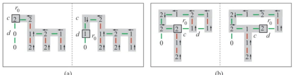
Since step 1 only affects c and d, it follows that at the beginning of step 2, a long gap in Sℓi+1must contain c, which becomes a 1-cell via PopOutLeaf (see Fig. 6a), or via Transfer (see Fig. 6b).
We now show that the loop in step 2 of TargetGrow iterates at most four times before our claim holds. Recall that, since Sℓi was root-clustered, children of c are either leaves, 2-cells, or their children have that property.
1 2 1 2 2 2 1 1 0 0 2 2 1 2 2 2 1 0 1 1 2 1 1 2 1 1 2 2 0 1 (a) 2 1 1 2 2 1 1 2 2 0 1 2 (b) d c d c d c c d r0 r0 r0 r0
Figure 6: DFS Root update (a) PopOutLeaf(c, d) (b) Transfer(c, d). Any Leaf Prune operation only trims visited 1-cell leaves from the tree and thus does not affect the root-clustered property of the tree. There are two cases for the number of ClusterStep applications required to terminate the loop:
1. Sℓi+1 was obtained via PopOutLeaf (step 1.1): In this case c and d are 1-cells at the beginning of step 2. If all children of c are leaves or 2-cells, then in the first iteration of ClusterStep, c will become a 2-cell again. Otherwise, since Sℓi was root-clustered, any non-leaf 1-cell child will become a 2-cell in the first iteration. Thus in the second iteration at the latest, c will become a 2-cell. Furthermore, just as described in Lemma 6, the subtree rooted at any child of c remains root-clustered after the first application of ClusterStep (in particular, for the highest-priority child which is the only one that changes). Similarly, by the time c becomes a 2-cell, the subtree rooted at c also becomes root-clustered. The third ClusterStep makes d a 2-cell root of a root-clustered tree, since all children of c must have been leaves or 2-cells to supply a module to c. The fourth ClusterStep makes c a 2-cell, which terminates the loop.
2. Sℓi+1 was obtained via Transfer (step 1.2): In this case d is already a 2-cell at the beginning of step 2 because of the Transfer opera-tion in step 1.2. If c remains a 2-cell during the transfer, then Sℓi+1 is already root-clustered and the loop condition is satisfied. If c is a 1-cell, arguments similar to case 1 imply that after one application of ClusterStep, Sℓi+1 is root-clustered. A second application of Clus-terStep makes c a 2-cell, which terminates the loop.
This concludes the proof.
Theorem 2. The InPlaceReconfiguration algorithm can be
Proof. By Lemma 5, phase 1 uses O(n) steps. Step 2 of
InPlaceReconfig-uration has O(n) iterations, since DFS has O(n) complexity. By Lemma 8, each iteration takes constant time.
5
Observations
Matching lower bound: Transforming a horizontal line of modules to a vertical line requires a linear number of parallel steps, if each module can only displace one other module and maximum velocity is constant.
3D: All of our techniques apply directly to 3D robots, once the top and bottom sides of cells are incorporated into our highest priority rule. None of our algorithms rely on the dimension being 2D. Once the primitive op-erations are set, every phase has a clear and direct extension to 3D. For instance, the 2D algorithm to construct a spanning tree of the robot can be extended in a straightforward way to 3D. The extension of our primitive op-erations is also trivial. Such opop-erations still involve an interaction between two adjacent cells. The extra dimension only adds the requirement that more adjacent cells must maintain connectivity to two given cells involved in a primitive operation. This poses no difficulties.
Reconfiguration of labeled robots: Our algorithms are essentially un-affected if labels are assigned to modules. This is of interest if a robot is to have specialized modules, equipped with cameras, drills, etc. In Tree-ToPath, assume that the partially constructed canonical path is sorted. Then a new module m can bubble/tunnel to its position by successive ap-plications of the Transfer primitive operation. When it gets there, the tail of the path (from m to leaf) must shift over. This is straightforward, involving propagation of one compressed unit, and does not interfere with other modules following m. At all times, m or its replacement makes steady progress towards the leaf.
For the in-place algorithm, T can first be constructed disregarding labels. A similar type of bubble-sort can then be applied, taking place within T . Telecube robots: The natural state of a telecube robot has atom arms contracted. There is no room to compress two modules into one cell. Thus an algorithm cannot commence with PushInLeaf operations, and it is not possible to physically exchange modules in adjacent cells while remaining in place. However, consider our first algorithm. We do not even need a SourceCluster phase, since all atoms are packed together. The root can transmit an instruction to a cell at maximum y-coordinate to act as root
and immediately push out two of its atoms. For the construction of V , all analysis follows. It seems that labeled atoms within a module might become separated (for example, if the module is at a junction in a tree). Thus an extra step is used, to collect the root atoms at the bottom of V .
Exact in-place reconfiguration is impossible for telecube robots if the modules are labeled. Thus the root cannot travel to any position within S. It might be possible to deal with this issue by requiring larger modules and designing a “reduced module shape” for the root (e.g., fewer atoms, using naturally expanded links). Instead, we could require that all modules have access to the map of T , which means any module can begin to expand T by filling adjacent 0-cells. Instead of backtracking or advancing through non-empty cells of T physically, the root can just tell its neighbors to take over. Eventually a new root module would expand T at a different connected component of 0-cells.
Other modular robots: It has been shown [Aloupis et al., 2009a]
that suitably constructed modules of other prototypes (e.g.,
M-TRAN [Kurokawa et al., 2007], ATRON [Jørgensen et al., 2004]) are
capable of simulating Crystalline atoms. Such modules may require 50-100 atoms to simulate one Crystalline atom, and the resulting shape is not compact. Nevertheless, the result in [Aloupis et al., 2009a] implies that our results here apply to large systems of other prototypes.
Acknowledgments. We thank the other participants of the 2008 Workshop
on Reconfiguration at the Bellairs Research Institute of McGill University for
providing a stimulating research environment. We also thank the reviewers of [Aloupis et al., 2008a] and Robotica for their constructive comments.
References
[Aloupis et al., 2009a] Aloupis, G., Benbernou, N., Damian, M., Demaine, E., Flatland, R., Iacono, J., and Wuhrer, S. (2009a). Efficient reconfigura-tion of lattice-based modular robots. In European Conference on Mobile
Robots, pages 81–86.
[Aloupis et al., 2008a] Aloupis, G., Collette, S., Damian, M., Demaine, E. D., El-Khechen, D., Flatland, R., Langerman, S., O’Rourke, J., Pin-ciu, V., Ramaswami, S., Sacrist´an, V., and Wuhrer, S. (2008a). Realistic reconfiguration of Crystalline and Telecube robots. In 8th International
[Aloupis et al., 2009b] Aloupis, G., Collette, S., Damian, M., Demaine, E. D., Flatland, R., Langerman, S., O’Rourke, J., Ramaswami, S., Sac-rist´an, V., and Wuhrer, S. (2009b). Linear reconfiguration of cube-style
modular robots. Computational Geometry: Theory and Applications,
42(6–7):652–663.
[Aloupis et al., 2008b] Aloupis, G., Collette, S., Demaine, E. D., Langer-man, S., Sacrist´an, V., and Wuhrer, S. (2008b). Reconfiguration of cube-style modular robots using O(log n) parallel moves. In Proc. Intl. Symp.
on Algorithms and Computation (ISAAC 2008), volume 5369 of LNCS,
pages 342–353.
[Aloupis et al., 2009c] Aloupis, G., Collette, S., Demaine, E. D.,
Langer-man, S., Sacrist´an, V., and Wuhrer, S. (2009c). Reconfiguration
of 3D crystalline robots in O(log n) parallel steps. Technical report
arXiv:0908.2440, 21 pages.
[Brener et al., 2008] Brener, N., Amar, F. B., and Bidaud, P. (2008). De-signing modular lattice systems with chiral space groups. International
Journal of Robotics Research, 27(3–4):279–297.
[Butler et al., 2001] Butler, Z., Byrnes, S., and Rus, D. (2001). Distributed motion planning for modular robots with unit-compressible modules. In
Proceedings of the IEEE/RSJ International Conference on Intelligent Robots and Systems (IROS).
[Butler et al., 2002] Butler, Z., Fitch, R., and Rus, D. (2002). Distributed control for unit-compressible robots: Goal-recognition, locomotion and splitting. IEEE/ASME Trans. on Mechatronics, 7(4):418–430.
[Butler et al., 2004] Butler, Z., Kotay, K., Rus, D., and Tomita, K. (2004). Generic decentralized control for lattice-based self-reconfigurable robots.
International Journal of Robotics Research, 23:919–937.
[Butler and Rus, 2003] Butler, Z. and Rus, D. (2003). Distributed planning and control for modular robots with unit-compressible modules. Intl.
Journal of Robotics Research, 22(9):699–715.
[Chiang and Chirikjian, 2001] Chiang, C.-J. and Chirikjian, G. (2001). Sim-ilarity metric with applications in modular robot motion planning.
Au-tonomous Robots, 10(1):91–106.
[Chirikjian, 1994] Chirikjian, G. (1994). Kinematics of a metamorphic
[Chirikjian et al., 1996] Chirikjian, G., Pamecha, A., and Ebert-Uphoff, I. (1996). Evaluating efficiency of self-reconfiguration in a class of modular robots. Journal of Robotic Systems, 13(5):317–338.
[Fukuda and Nakagawa, 1988] Fukuda, T. and Nakagawa, S. (1988). Ap-proach to the dynamically reconigurable robotic system. Journal of
In-telligent and Robotic Systems, 1(1):55–72.
[Hosokawa et al., 1998] Hosokawa, K., Tsujimori, T., Fujii, T., Kaetsu, H., Asama, H., Kuroda, Y., and Endo, I. (1998). Self-organizing collec-tive robots with morphogenesis in a vertical plane. In Proceedings of
the IEEE International Conference on Robotics and Automation (ICRA),
pages 2858–2863.
[Jørgensen et al., 2004] Jørgensen, M. W., Østergaard, E. H., and Lund, H. H. (2004). Modular ATRON: Modules for a self-reconfigurable robot. In Proc. of the International Conference on Intelligient Robots and
Sys-tems, pages 2068–2073.
[Kotay and Rus, 2000] Kotay, K. and Rus, D. (2000). Algorithms for self-reconfiguring molecule motion planning. In Proceedings of the
Interna-tional Conference on Intelligent Robots and Systems, pages 2184–2193.
[Kurokawa et al., 2007] Kurokawa, H., Tomita, K., Kamimura, A., Kokaji, S., Hasuo, T., and Murata, S. (2007). Self-reconfigurable modular robot m-tran: distributed control and communication. In RoboComm ’07:
Pro-ceedings of the 1st international conference on Robot communication and coordination, pages 1–7, Piscataway, NJ, USA. IEEE Press.
[Kurokawa et al., 2008] Kurokawa, H., Tomita, K., Kamimura, A., Kokaji, S., Hasuo, T., and Murata, S. (2008). Distributed self-reconfiguration of M-TRAN III modular robotic system. International Journal of Robotics
Research, 27:373–386.
[Murata and Kurokawa, 2007] Murata, S. and Kurokawa, H. (2007). Self-reconfigurable robots: Shape-changing cellular robots can exceed conven-tional robot flexibility. IEEE Robotics & Automation Magazine, 14(1):43– 52.
[Murata et al., 1994] Murata, S., Kurokawa, H., and Kokaji, S. (1994). Self-assembling machine. In Proc. IEEE Int. Conf. Robot. Automat., pages 441–448.
[Pamecha et al., 1996] Pamecha, A., Chiang, C., Stein, D., and Chirikjian, G. (1996). Design and implementation of metamorphic robots. In
Proceed-ings of the ASME Design Engineering Technical Conference and Comput-ers in Engineering Conference.
[Pamecha et al., 1997] Pamecha, A., Ebert-Uphoff, I., and Chirikjian, G. (1997). Useful metrics for modular robot motion planning. IEEE
Trans-actions on Robotics and Automation, 13(4):531–545.
[Reif and Slee, 2007] Reif, J. H. and Slee, S. (2007). Optimal kinodynamic motion planning for self-reconfigurable robots between arbitrary 2D con-figurations. In Robotics: Science and Systems Conference, Georgia
Insti-tute of Technology.
[Rus and Vona, 2001] Rus, D. and Vona, M. (2001). Crystalline robots: Self-reconfiguration with compressible unit modules. Autonomous Robots, 10(1):107–124.
[Salemi et al., 2003] Salemi, B., Will, P., and Shen, W.-M. (2003). Dis-tributed task negotiation in modular robots. Journal of the Robotics
So-ciety of Japan, Special Issue on “Modular Robots”, 21(8):32–39.
[Stoy, 2006] Stoy, K. (2006). Using cellular automata and gradients to con-trol self-reconfiguration. Robotics and Autonomous Systems, 54 (special issue IAS-04):135–141.
[Suh et al., 2002] Suh, J. W., Homans, S. B., and Yim, M. (2002). Tele-cubes: Mechanical design of a module for self-reconfigurable robotics. In
Proc. of the IEEE Intl. Conf. on Robotics and Automation, pages 4095–
4101.
[ ¨Unsal et al., 2000] ¨Unsal, C., Kilite, H., Patton, M., and Khosla, P. (2000). Motion planning for a modular self-reconfiguring robotic system. In
Pro-ceedings of the 5th International Symposium on Distributed Autonomous Robotic Systems.
[Vassilvitskii et al., 2002] Vassilvitskii, S., Yim, M., and Suh, J. (2002). A complete, local and parallel reconfiguration algorithm for cube style mod-ular robots. In Proc. of the IEEE Intl. Conf. on Robotics and Automation, pages 117–122.
[Walter et al., 2002] Walter, J. E., Tsai, E. M., and Amato, N. M. (2002). Choosing good paths for fast distributed reconfiguration of hexagonal
metamorphic robots. In Proceedings of the IEEE International Conference
on Robotics and Automation (ICRA), pages 102–109.
[Yim, 1994] Yim, M. (1994). New locomotion gaits. In Proc. IEEE Int.
Conf. Robot. Automat.
[Yim et al., 2000] Yim, M., Duff, D. G., and Roufas, K. D. (2000). Polybot: a modular reconfigurable robot. In Proc. of the 2000 IEEE International
Conference on Robotics and Automation, pages 514–520.
[Yim et al., 2007] Yim, M., Shen, W.-M., Salemi, B., Rus, D., Moll, M., Lipson, H., Klavins, E., and Chirikjian, G. S. (2007). Modular self-reconfigurable robots systems: Challenges and opportunities for the fu-ture. IEEE Robotics & Automation Magazine, 14(1):43–52.
[Yoshida et al., 2002] Yoshida, E., Murata, S., Kamimura, A., Tomita, K., Kurokawa, H., and Kokaji, S. (2002). A self-reconfigurable modular robot: Reconfiguration planning and experiments. The International Journal of
Appendix
PushInLeaf and PopOutLeaf
(a) (b) (c) (d) (e)
(f) (g) (h) (i) (j)
(k) (l) (m) (n) (o)
Transfer
(a) (b) (c) (d) (e)
(f) (g) (h) (i) (j)
(k) (l) (m) (n) (o)
(p) (q) (r) (s) (t)
Figure 8: Details of the positioning step of the primitive operation
Transfer(m, q). Before being sent to the lattice position of q, the module m is rotated within its lattice cell, in order to face q.
(a) (b) (c) (d) (e)
(f) (g) (h) (i) (j)
(k) (l) (m) (n) (o)
(a) (b) (c) (d) (e)
(f) (g) (h) (i) (j)
(k) (l) (m) (n) (o)
(p) (q) (r) (s) (t)
(u) (v) (w) (x) (y)
Figure 10: Details of the Exchange step of the primitive operation Trans-fer.
Switch
(a) (b) (c) (d) (e)
(f) (g) (h) (i) (j)
(k) (l) (m) (n) (o)
(p) (q) (r) (s) (t)