Atoms of recognition in human and computer vision

Atoms of recognition in human and computer vision

The MIT Faculty has made this article openly available.

Please share

how this access benefits you. Your story matters.

Citation

Ullman, Shimon et al. “Atoms of Recognition in Human and

Computer Vision.” Proceedings of the National Academy of Sciences

113.10 (2016): 2744–2749. © 2016 National Academy of Sciences

As Published

http://dx.doi.org/10.1073/pnas.1513198113

Publisher

National Academy of Sciences (U.S.)

Version

Final published version

Citable link

http://hdl.handle.net/1721.1/106502

Terms of Use

Article is made available in accordance with the publisher's

policy and may be subject to US copyright law. Please refer to the

publisher's site for terms of use.

Atoms of recognition in human and computer vision

Shimon Ullman

, Liav Assif

, Ethan Fetaya

, and Daniel Harari

a_{Department of Computer Science and Applied Mathematics, Weizmann Institute of Science, Rehovot 7610001, Israel;}b_{Department of Brain and Cognitive}

Sciences, Massachusetts Institute of Technology, Cambridge, MA 02139; andc_{McGovern Institute for Brain Research, Cambridge, MA 02139}

Edited by Michael E. Goldberg, Columbia University College of Physicians, New York, NY, and approved January 11, 2016 (received for review July 8, 2015) Discovering the visual features and representations used by the

brain to recognize objects is a central problem in the study of vision. Recently, neural network models of visual object recognition, includ-ing biological and deep network models, have shown remarkable progress and have begun to rival human performance in some chal-lenging tasks. These models are trained on image examples and learn to extract features and representations and to use them for categorization. It remains unclear, however, whether the represen-tations and learning processes discovered by current models are similar to those used by the human visual system. Here we show, by introducing and using minimal recognizable images, that the human visual system uses features and processes that are not used by current models and that are critical for recognition. We found by psychophysical studies that at the level of minimal recognizable images a minute change in the image can have a drastic effect on recognition, thus identifying features that are critical for the task. Simulations then showed that current models cannot explain this sensitivity to precise feature configurations and, more generally, do not learn to recognize minimal images at a human level. The role of the features shown here is revealed uniquely at the minimal level, where the contribution of each feature is essential. A full under-standing of the learning and use of such features will extend our understanding of visual recognition and its cortical mechanisms and will enhance the capacity of computational models to learn from visual experience and to deal with recognition and detailed image interpretation.

object recognition

|

|

|

|

T

he human visual system makes highly effective use of limited

information (1, 2). As shown below (Fig. 1 and

Figs. S1

and

S2

), it can recognize consistently subconfigurations that are

se-verely reduced in size or resolution. Effective recognition of

reduced configurations is desirable for dealing with image

vari-ability: Images of a given category are highly variable, making

recognition difficult, but this variability is reduced at the level of

recognizable but minimal subconfigurations (Fig. 1B). Minimal

recognizable configurations (MIRCs) are useful for effective

recognition, but, as shown below, they also are computationally

challenging because each MIRC is nonredundant and therefore

requires the effective use of all available information. We use

them here as sensitive tools to identify fundamental limitations

of existing models of visual recognition and directions for

essential extensions.

A MIRC is defined as an image patch that can be reliably

recognized by human observers and which is minimal in that

fur-ther reduction in eifur-ther size or resolution makes the patch

un-recognizable (below criterion) (Methods). To discover MIRCs, we

conducted a large-scale psychophysical experiment for

classifica-tion. We started from 10 greyscale images, each showing an object

from a different class (

Fig. S3

), and tested a large hierarchy of

patches at different positions and decreasing size and resolution.

Each patch in this hierarchy has five descendants, obtained by

ei-ther cropping the image or reducing its resolution (Fig. 2). If an

image patch was recognizable, we continued to test the recognition

of its descendants by additional observers. A recognizable patch

in this hierarchy is identified as a MIRC if none of its five

descendants reaches a recognition criterion (50% recognition;

re-sults are insensitive to criterion) (Methods and

Fig. S4

). Each

hu-man subject viewed a single patch from each image with unlimited

viewing time and was not tested again. Testing was conducted

online using the Amazon Mechanical Turk (MTurk) (3, 4) with

about 14,000 subjects viewing 3,553 different patches combined

with controls for consistency and presentation size (Methods). The

size of the patches was measured in image samples, i.e., the

number of samples required to represent the image without

re-dundancy [twice the image frequency cutoff (5)]. For presentation

to subjects, all patches were scaled to 100

× 100 pixels by standard

interpolation; this scaling increases the size of the presented image

smoothly without adding or losing information.

Results

Discovered MIRCs.

Each of the 10 original images was covered by

multiple MIRCs (15.1

± 7.6 per image, excluding highly

over-lapping MIRCs) (Methods) at different positions and sizes (Fig. 3

and

Figs. S1

and

S2

). The resolution (measured in image

sam-ples) was small (14.92

± 5.2 samples) (Fig. 3A), with some

cor-relation (0.46) between resolution and size (the fraction of the

object covered). Because each MIRC is recognizable on its own,

this coverage provides robustness to occlusion and distortions at

the object level, because some MIRCs may be occluded and the

overall object may distort and still be recognized by a subset of

recognizable MIRCs.

The transition in recognition rate from a MIRC image to a

nonrecognizable descendant (termed a

“sub-MIRC”) is typically

sharp: A surprisingly small change at the MIRC level can make

it unrecognizable (Fig. 4). The drop in recognition rate was

quantified by measuring a recognition gradient, defined as the

maximal difference in recognition rate between the MIRC and

Significance

Discovering the visual features and representations used by the brain to recognize objects is a central problem in the study of vision. Recent successes in computational models of visual rec-ognition naturally raise the question: Do computer systems and the human brain use similar or different computations? We show by combining a novel method (minimal images) and simulations that the human recognition system uses features and learning processes, which are critical for recognition, but are not used by current models. The study uses a“phase transition” phenome-non in minimal images, in which minor changes to the image have a drastic effect on its recognition. The results show fun-damental limitations of current approaches and suggest direc-tions to produce more realistic and better-performing models.

Author contributions: S.U., L.A., E.F., and D.H. designed research; L.A. and D.H. performed research; L.A. and D.H. analyzed data; and S.U., L.A., and D.H. wrote the paper. The authors declare no conflict of interest.

This article is a PNAS Direct Submission.

Freely available online through the PNAS open access option.

1_{S.U., L.A., and D.H. contributed equally to this work.}

2_{To whom correspondence should be addressed. Email: shimon.ullman@weizmann.ac.il.}

This article contains supporting information online atwww.pnas.org/lookup/suppl/doi:10. 1073/pnas.1513198113/-/DCSupplemental.

NEUROSCI

its five descendants. The average gradient was 0.57

± 0.11,

in-dicating that much of the drop from full to no recognition occurs

for a small change at the MIRC level (the MIRC itself or one

level above, where the gradient also was found to be high). The

examples in Fig. 4 illustrate how small changes at the MIRC level

can have a dramatic effect on recognition rates. These changes

disrupt visual features to which the recognition system is

sensi-tive (6–9); these features are present in the MIRCs but not in the

sub-MIRCs. Crucially, the role of these features is revealed

uniquely at the MIRC level, because information is more

re-dundant in the full-object image, and a similar loss of features

will have a small effect. By comparing recognition rates of

models at the MIRC and sub-MIRC levels, we were able to

test computationally whether current models of human and

computer vision extract and use similar visual features and to test

the ability of recognition models to recognize minimal images at

a human level. The models in our testing included HMAX (10),

a high-performing biological model of the primate ventral

stream, along with four state-of-the-art computer vision models:

(i) the Deformable Part Model (DPM) (11); (ii) support vector

machines (SVM) applied to histograms of gradients (HOG)

representations (12); (iii) extended Bag-of-Words (BOW) (13,

14); and (iv) deep convolutional networks (Methods) (15). All are

among the top-performing schemes in standard evaluations (16).

Training Models on Full-Object Images.

We first tested the models

after training with full-object images. Each of the classification

schemes was trained by a set of class and nonclass images to

produce a classifier that then could be applied to novel test

images. For each of the 10 objects in the original images we used

60 class images and an average of 727,000 nonclass images

(Methods). Results did not change by increasing the number of

training class images to 472 (Methods and

SI Methods

). The class

examples showed full-object images similar in shape and viewing

direction to the stimuli in the psychophysical test (

Fig. S5

).

After training, all classifiers showed good classification results

when applied to novel full-object images, as is consistent with the

reported results for these classifiers [average precision (AP)

=

0.84

± 0.19 across classes]. The trained classifiers then were

tested on MIRC and sub-MIRC images from the human testing,

with the image patch shown in its original location and size and

surrounded by an average gray image. The first objective was to

test whether the sharp transition shown in human recognition

between images at the MIRC level and their descendant

sub-MIRCs is reproduced by any of the models (the accuracy of

MIRC detection is discussed separately below). An average of

10 MIRC level patches per class and 16 of their similar

sub-MIRCs were selected for testing, together with 246,000

non-class patches. These MIRCs represent about 62% of the total

number of MIRCs and were selected to have human

recog-nition rates above 65% for MIRCs and below 20% for

sub-MIRCs (Methods). To test the recognition gap, we set the

acceptance threshold of the classifier to match the average

hu-man recognition rate for the class (e.g., 81% for the MIRC-level

patches from the original image of an eye) (Methods and

Fig. S6

)

and then compared the percentage of MIRCs vs. sub-MIRCs

that exceeded the classifier’s acceptance threshold (results were

insensitive to threshold setting over the range of recognition

rates 0.5–0.9).

We computed the gap between MIRC and sub-MIRC

recog-nition rates for the 10 classes and the different models and

compared the gaps in the models’ and human recognition rates.

None of the models came close to replicating the large drop

shown in human recognition (average gap 0.14

± 0.24 for models

vs. 0.71

± 0.05 for humans) (

Fig. S7A

). The difference between

the models’ and human gaps was highly significant for all

com-puter-version models (P

< 1.64 × 10

for all classifiers, n

=

10 classes, df

= 9, average 16 pairs per class, one-tailed paired

t test). HMAX (10) showed similar results (gap 0.21

± 0.23). The

gap is small because, for the models, the representations of

MIRCs and sub-MIRCs are closely similar, and consequently

the recognition scores of MIRCs and sub-MIRCs are not well

separated.

It should be noted that recognition rates by themselves do not

directly reflect the accuracy of the learned classifier: A classifier

can recognize a large fraction of MIRC and sub-MIRC examples

by setting a low acceptance threshold, but doing so will result in

the erroneous acceptance of nonclass images. In all models, the

accuracy of MIRC recognition (AP 0.07

± 0.10) (

Fig. S7B

) was

low compared with the recognition of full objects (AP 0.84

±

0.19) and was still lower for sub-MIRCs (0.02

± 0.05). At these

low MIRC recognition rates the system will be hampered by a

large number of false detections.

Fig. 1. Reduced configurations. (A) Configurations that are reduced in size (Left) or resolution (Right) can often be recognized on their own. (B) The full images (Upper Row) are highly variable. Recognition of the common action can be obtained from local configurations (Lower Row), in which variability is reduced.

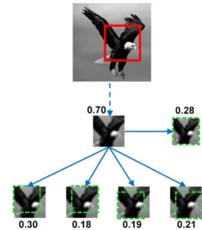
Fig. 2. MIRCs discovery. If an image patch was recognized by human sub-jects, five descendants were presented to additional observers: Four were obtained by cropping 20% of the image (Bottom Row) and one by 20% re-duced resolution (Middle Row, Right). The process was repeated on all descendants until none of the descendants reached recognition criterion (50%). Detailed examples are shown inFig. S4. The numbers next to each image indicate the fraction of subjects that correctly recognized the image.

A conceivable possibility is that the performance of model

networks applied to minimal images could be improved to the

human level by increasing the size of the model network or the

number of explicitly or implicitly labeled training data. Our tests

suggest that although these possibilities cannot be ruled out, they

appear unlikely to be sufficient. In terms of network size,

dou-bling the number of levels (see ref. 17 vs. ref. 18) did not improve

MIRC recognition performance. Regarding training examples,

our testing included two network models (17, 18) that were

trained previously on 1.2 million examples from 1,000 categories,

including 7 of our 10 classes, but the recognition gap and

accu-racy of these models applied to MIRC images were similar to

those in the other models.

We considered the possibility that the models are trained for a

binary decision, class vs. nonclass, whereas humans recognize

multiple classes simultaneously, but we found that the gap is

similar and somewhat smaller for multiclass recognition (Methods

and

SI Methods

). We also examined responses of intermediate

units in the network models and found that results for the

best-performing intermediate layers were similar to the results of the

network’s standard top-level output (Methods).

Training Models on Image Patches.

In a further test we simplified

the learning task by training the models directly with images at

the MIRC level rather than with full-object images. Class

ex-amples were taken from the same class images used in full-object

learning but using local regions at the true MIRC locations and

approximate scale (average 46 examples per class) that had been

verified empirically to be recognizable on their own (Methods

and

Fig. S8

). After training, the models’ accuracy in recognizing

MIRC images was significantly higher than in learning from

full-object images but still was low in absolute terms and in

com-parison with human recognition (AP 0.74

± 0.21 for training on

patches vs. 0.07

± 0.10 for training on full-object images) (

SI

Methods

,

Training Object on Image Patches

and

SI Methods

,

Human Binary Classification Test

). The gap in recognition

be-tween MIRC and sub-MIRC images remained low (0.20

± 0.15

averaged over pairs and classifiers) and was significantly lower than

the human gap for all classifiers (P

< 1.87 × 10

for all classifiers,

n

= 10 classes, df = 9, one-tailed paired t test) (Methods and

SI Methods

).

Detailed Internal Interpretation.

An additional limitation of current

modeling compared with human vision is the ability to perform

a detailed internal interpretation of MIRC images. Although

MIRCs are

“atomic” in the sense that their partial images become

unrecognizable, our tests showed that humans can consistently

recognize multiple components internal to the MIRC (Methods

and Fig. 3C). Such internal interpretation is beyond the capacities

of current neural network models, and it can contribute to accurate

recognition, because a false detection could be rejected if it does

not have the expected internal interpretation.

Discussion

The results indicate that the human visual system uses features

and processes that current models do not. As a result, humans are

better at recognizing minimal images, and they exhibit a sharp drop

in recognition at the MIRC level, which is not replicated in models.

The sharp drop at the MIRC level also suggests that different

human observers share similar visual representations, because the

transitions occur for the same images, regardless of individual

vi-sual experience. An interesting open question is whether the

ad-ditional features and processes are used in the visual system as a

part of the cortical feed-forward process (19) or by a top-down

process (20–23), which currently is missing from the purely

feed-forward computational models.

We hypothesize based on initial computational modeling that

top-down processes are likely to be involved. The reason is that detailed

interpretation appears to require features and interrelations that are

relatively complex and are class-specific, in the sense that their

presence depends on a specific class and location (24). This

appli-cation of top-down processes naturally divides the recognition

pro-cess into two main stages: The first leads to the initial activation

of class candidates, which is incomplete and with limited accuracy.

The activated representations then trigger the application of

class-specific interpretation and validation processes, which recover

richer and more accurate interpretation of the visible scene.

A further study of the extraction and use of such features by

the brain, combining physiological recordings and modeling, will

extend our understanding of visual recognition and improve the

capacity of computational models to deal with recognition and

detailed image interpretation.

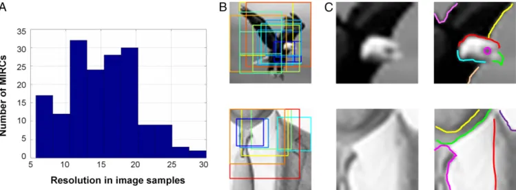
Fig. 3. (A) Distribution of MIRCs’ resolution (measured in image samples), average 14.92 ± 5.2 samples. (B) MIRCs’ coverage. The original images are covered by multiple MIRCs at different positions, sizes, and resolutions. Each colored frame outlines a MIRC (which may be at a reduced resolution). Because each MIRC is recognizable on its own, this coverage provides robustness to occlusion and transformations. (C) Detailed internal interpretation labeled by subjects (n= 30) (Methods). Suit image parts: tie, shirt, jacket, chin, neck. Eagle image parts: eye, beak, head, wing, body, sky.

NEUROSCI

Methods

Data for MIRC Discovery. A set of 10 images was used to discover MIRCs in the psychophysics experiment. These images of objects and object parts (one image from each of 10 classes) were used to generate the stimuli for the human tests (Fig. S3). Each image was of size 50× 50 image samples (cutoff frequency of 25 cycles per image).

Data for Training and Testing on Full-Object Images. A set of 600 images was used for training models on full-object images. For each of the 10 images in the psychophysical experiment, 60 training class images were obtained (from Google images, Flickr) by selecting similar images as measured by their HOG (12) representations; examples are given inFig. S5. The images were of full objects (e.g., the side view of a car rather than the door only). These images provided positive class examples on which the classifiers were trained, using 30–50 images for training; the rest of the images were used for testing. (Different training/testing splits yielded similar results.) We also tested the effect of increasing the number of positive examples to 472 (split into 342 training and 130 testing) on three classes (horse, bicycle, and airplane) for which large datasets are available in PASCAL (16) and ImageNet (25). For the convolutional neural network (CNN) multiclass model used (15), the number of training images was 1.2 million from 1,000 categories, including 7 of the 10 classes used in our experiment.

To introduce some size variations, two sizes differing by 20% were used for each image. The size of the full-object images was scaled so that the part used in the human experiment (e.g., the car door) was 50× 50 image samples (with 20% variation). For use in the different classifiers, the images were in-terpolated to match the format used by the specific implementations [e.g., 227× 227 for regions with CNN (RCNN)] (15). The negative images were taken from PASCAL VOC 2011 (host.robots.ox.ac.uk/pascal/VOC/voc2011/ index.html), an average of 727,440 nonclass image regions per class extracted from 2,260 images used in training and 246,000 image regions extracted from a different set of 2,260 images used for testing. The number of non-class images is larger than the non-class images used in training and testing, because this difference is also common under natural viewing conditions of class and nonclass images.

Data for Training and Testing on Image Patches. The image patches used for training and testing were taken from the same 600 images used in full-object image training, but local regions at the true location and size of MIRCs and sub-MIRCs (called the“siblings dataset”) (Fig. S8) were used. Patches were scaled to a common size for each of the classifiers. An average of 46 image patches from each class (23 MIRCs and 23 sub-MIRC siblings) were used as positive class examples, together with a pool of 1,734,000 random nonclass patches of similar sizes taken from 2,260 nonclass images. Negative nonclass images during testing were 225,000 random patches from another set of 2,260 images.

Model Versions and Parameters. The versions and parameters of the four classification models used were as follows. The HOG (12) model used the implementation of VLFeat version 0.9.17 (www.vlfeat.org/), an open and portable library of computer vision algorithms, using cell size 8. For BOW we used the selective search method (26) using the implementation of VLFeat with an encoding of VLAD (vector of locally aggregated descriptors) (14, 27), a dictionary of size 20, a 3× 3 grid division, and dense SIFT (28) descriptor. DPM (11) used latest version (release 5,www.cs.berkeley.edu/∼rbg/latent/) with a single mode. For RCNN we used a pretrained network (15), which uses the last feature layer of the deep network trained on ImageNet (17) as a descriptor. Additional deep-network models tested were a model developed for recognizing small (32× 32) images (29), and Very Deep Convolutional Network (18), which was adapted for recognizing small images. HMAX (10) used the implementation of Cortical Network Simulator (CNS) (30) with six scales, a buffer size of 640× 640, and a base size of 384 × 384.

MIRCs Discovery Experiment. This psychophysics experiment identified MIRCs within the original 10 images at different sizes and resolutions (by steps of 20%). At each trial, a single image patch from each of the 10 images, starting with the full-object image, was presented to observers. If a patch was rec-ognizable, five descendants were presented to additional observers; four of the descendants were obtained by cropping (by 20%) at one corner, and one was a reduced resolution of the full patch. For instance, the 50× 50 original image produced four cropped images of size 40× 40 samples, together with a 40× 40 reduced-resolution copy of the original (Fig. 2). For presentation, all patches were rescaled to 100× 100 pixels by image interpolation so that the size of the presented image was increased without the addition or loss of information. A search algorithm was used to accelerate the search, based on the following monotonicity assumption: If a patch P is recognizable, then larger patches or P at a higher resolution will also be recognized; similarly, if P is not recognized, then a cropped or reduced resolution version also will be unrecognized.

A recognizable patch was identified as a MIRC (Fig. 2 andFig. S4) if none of its five descendants reached a recognition criterion of 50%. (The accep-tance threshold has only a small effect on the final MIRCs because of the sharp gradient in recognition rate at the MIRC level.) Each subject viewed a single patch from each image and was not tested again. The full procedure required a large number of subjects (a total of 14,008 different subjects; average age 31.5 y; 52% males). Testing was conducted online using the Amazon MTurk platform (3, 4). Each subject viewed a single patch from each of the 10 original images (i.e., class images) and one“catch” image (a highly recognizable image for control purposes, as explained below). Subjects were given the following instructions:“Below are 11 images of objects and object parts. For each image type the name of the object or part in the image. If you do not recognize anything type‘none’.” Presentation time was not limited, and the subject responded by typing the labels. All experiments and Fig. 4. Recognition gradient. A small change in images at the MIRC level can cause a large drop in the human recognition rate. Shown are examples of MIRCs (A and B) and corresponding sub-MIRCs (A* and B*). The numbers under each image indicate the human recognition rate. The average drop in recognition for these pairs is 0.67.

procedures were approved by the institutional review boards of the Weizmann Institute of Science, Rehovot, Israel. All participants gave informed consent before starting the experiments.

In comparative studies MTurk has been shown to produce reliable re-peatable behavior data, and many classic findings in cognitive psychology have been replicated using data collected online (4). The testing was ac-companied by the following controls. To verify comprehension (4), each test included a highly recognizable image; responses were rejected if this catch image was not correctly recognized (rejection rate<1%). We tested the consistency of the responses by dividing the responses of 30 subjects for each of 1,419 image patches into two groups of 15 workers per group and compared responses across groups. Correlation was 0.91, and the difference was not significant (n= 1,419, P = 0.29, two-tailed paired t test), showing that the procedure yields consistent recognition rates. A labo-ratory test under controlled conditions replicated the recognition results obtained in the online study: Recognition rates for 20 MIRCs/sub-MIRCs in the online and laboratory studies had correlation of 0.84, and all MIRC/ sub-MIRC pairs that were statistically different in the online study were also statistically different in the laboratory study. Because viewing size cannot be accurately controlled in the online trials, we verified in a lab-oratory experiment that recognition rates do not change significantly over 1–4° of visual angle.

Subjects were excluded from the analysis if they failed to label all 10 class image patches or failed to label the catch image correctly (failure rate, 2.2%). The average number of valid responses was 23.7 per patch tested. A response was scored as 1 if it gave the correct object name and as 0 otherwise. Some answers required decisions regarding the use of related terms, e.g., whether “bee” instead of “fly” would be accepted. The decision was based on the WordNet hierarchy (31): We allowed sister terms that have the same direct parent (hypernym) or two levels up. For instance,“’cow” was accepted as a label for“horse,” but “dog” or “bear” was not. Part-names were accepted if they correctly labeled the visible object in the partial image (e.g.,“wheel” in bicycle,“tie” in suit image, “jet engine” for the airplane part); descriptions that did not name specific objects (e.g.,“cloth,” “an animal part,” “wire”) were not accepted.

Training Models on Full-Object Images. Training was done for each of the classifiers using the training data, except for the multiclass CNN classifier (15), which was pretrained on 1,000 object categories based on ImageNet (27). Classifiers then were tested on novel full images using standard procedures, followed by testing on MIRC and sub-MIRC test images.

Detection of MIRCs and sub-MIRCs. An average of 10 MIRC level patches and 16 of their sub-MIRCs were selected for testing per class. These MIRCs, which represent about 62% of the total number of MIRCs, were selected based on their recognition gap (human recognition rate above 65% for MIRC level patches and below 20% for their sub-MIRCs) and image similarity between MIRCs and sub-MIRCs (as measured by overlap of image con-tours); the same MIRC could have several sub-MIRCs. The tested patches were placed in their original size and location on a gray background; for example, an eye MIRC with a size of 20× 20 samples (obtained in the human experiment) was placed on gray background image at the original eye location.

Computing the recognition gap. To obtain the classification results of a model, the model’s classification score was compared against an acceptance threshold (32), and scores above threshold were considered detections. After training a model classifier, we set its acceptance threshold to pro-duce the same recognition rate of MIRC patches as the human recognition rate for the same class. For example, for the eye class, the average human recognition rate of MIRCs was 0.81; the model threshold was set so that the model’s recognition rate of MIRCs was 0.8. We then found the rec-ognition rate of the sub-MIRCs using this threshold. The difference be-tween the recognition rates of MIRCs and sub-MIRCs is the classifier’s recognition gap. (Fig. S6). In an additional test we tested the gap while varying the threshold to produce recognition rates in the range 0.5–0.9 and found that the results were insensitive to the setting of the models’ threshold. For the computational models, the scores of sub-MIRCs were intermixed with the scores of MIRCs, limiting the recognition gap between the two, as compared with human vision.

Multiclass estimation. The computational models are trained for a binary de-cision, class vs. nonclass, whereas humans recognize multiple classes simul-taneously. This multiclass task can lead to cases in which classification results of the correct class may be overridden by a competing class. The multiclass effect was evaluated in two ways. The first was by simulations, using sta-tistics from the human test, and the second was by direct multiclass classi-fication, using the CNN multiclass classifier (15). The mean rate of giving a

wrong-class response (rather than producing the‘none’ label) in the hu-man experiments ranged from 37% for the lowest recognition rates to 4% at highest recognition rates. The effect of multiclass decision on the binary classifier was simulated by allowing each tested MIRC or sub-MIRC to be overridden by a class other than the tested category, with a probability that varied linearly between 4% for the highest-scoring results and 37% for the lowest-scoring results in each class. The gap between MIRC and sub-MIRC recognition was computed as before, but with the additional misclassifications produced by the simulated multiclass effect. The average recognition gap between MIRCs and sub-MIRCS was 0.11± 0.16 for mul-ticlass vs. 0.14± 0.24 for binary classification. The multiclass effect was expected to be small because the scores in the models for the MIRCs and sub-MIRCs were highly intermixed. Multiclass classification also was tested directly using the CNN model that was trained previously on 1,000 cate-gories (15), including 7 of our 10 classes. Given a test image, the model produces the probability that this image belongs to each of the network categories. The score for each MIRC and sub-MIRC is the probability of the tested class given the test image (e.g., the probability of the airplane class given an airplane MIRC or sub-MIRC). The average gap for the seven classes was small (0.14 ± 0.35) with no significant difference between MIRCs and sub-MIRCs.

Classification accuracy was computed by the AP of the classifier, the standard evaluation measure for classifiers (16). To compare the AP in the full object, the MIRC, and the sub-MIRC classification tasks, we normalize the results to the same number of positive and negative examples across the three test sets.

Intermediate units. In training and testing the HMAX model (10), we examined whether any intermediate units in the network developed a specific re-sponse to a MIRC image during training. Following full-object image train-ing, we tested the responses of all units at all layers of the network to MIRC patches and nonclass patches. We identified the best-performing unit at each of the network’s layers (denoted S1, C1, S2, C2, S3, and C3) in terms of its precision in recognizing a particular MIRC type. On this set, the AP at the network output was 94± 9% for full-object images and 19 ± 19% for MIRCs. For units with best AP across the network, results were low, but still were higher than the single C3 output unit: AP= 40 ± 24% at the S2 level, 44 ± 27% at the C2 level, and 39± 21% at the S3 level.

Training Models on Image Patches. The classifiers used in the full-object image experiment were trained and tested for image patches. For the RCNN model (15), the test patch was either in its original size or was scaled up to the network size of 227× 227. In addition, the deep network model (29) and Very Deep Convolutional Network model (18), adapted for recog-nizing small images, were tested also. Training and testing procedures were the same as for the full-object image test, repeating in five-folds, each using 37 patches for training and nine for testing. Before the computa-tional testing, we measured in psychophysical testing the recognition rates of all the patches from all class images to compare human and model rec-ognition rates directly on the same image (see examples inFig. S8). After training, we compared the recognition rates of MIRCs and sub-MIRCs by the different models and their recognition accuracy, as in the full-object image test.

We also tested intermediate units in a deep convolutional network (18) by selecting a layer (the eighth of 19) in which units’ receptive field sizes best approximated the size of MIRC patches. The activation levels of all units in this layer were used as an input layer to an SVM classifier, replacing the usual top-level layer. The gap and accuracy of MIRC classification based on the intermediate units were not significantly changed compared with the results of the networks’ tested top-level output.

Internal Interpretation Labeling. Subjects (n= 30) were presented with a MIRC image in which a red arrow pointed to a location in an image (e.g., the beak of the eagle) and were asked to name the indicated location. Alternatively, one side of a contour was colored red, and subjects produced two labels for the two sides of the contour (e.g., ship and sea). In both alternatives the subjects also were asked to name the object they saw in the image (without the markings).

ACKNOWLEDGMENTS. We thank Michal Wolf for help with data collection and Guy Ben-Yosef, Leyla Isik, Ellen Hildreth, Elias Issa, Gabriel Kreiman, and Tomaso Poggio for discussions and comments. This work was sup-ported by European Research Council Advanced Grant“Digital Baby” (to S.U.) and in part by the Center for Brains, Minds and Machines, funded by National Science Foundation Science and Technology Centers Award CCF-1231216.

NEUROSCI

1. Torralba A, Fergus R, Freeman WT (2008) 80 million tiny images: A large data set for nonparametric object and scene recognition. IEEE Trans Pattern Anal Mach Intell 30(11):1958–1970.

2. Bourdev L, et al. (2009) Poselets: Body part detectors trained using 3D human pose annotations. Proceedings of IEEE 12th International Conference on Computer Vision (ICCV), Kyoto, Japan September 27 - October 4, 2009 (IEEE, New York).

3. Buhrmester M, Kwang T, Gosling SD (2011) Amazon’s mechanical Turk: A new source of inexpensive, yet high-quality, data? Perspect Psychol Sci 6(1):3–5.

4. Crump MJC, McDonnell JV, Gureckis TM (2013) Evaluating Amazon’s mechanical Turk as a tool for experimental behavioral research. PLoS One 8(3):e57410.

5. Bracewell RN (1999) The Fourier Transform and Its Applications (McGraw-Hill, Sin-gapore), 3rd Ed.

6. Desimone R, Albright TD, Gross CG, Bruce C (1984) Stimulus-selective properties of inferior temporal neurons in the macaque. J Neurosci 4(8):2051–2062.

7. Fujita I, Tanaka K, Ito M, Cheng K (1992) Columns for visual features of objects in monkey inferotemporal cortex. Nature 360(6402):343–346.

8. Gallant JL, Braun J, Van Essen DC (1993) Selectivity for polar, hyperbolic, and Cartesian gratings in macaque visual cortex. Science 259(5091):100–103.

9. Kourtzi Z, Connor CE (2011) Neural representations for object perception: Structure, category, and adaptive coding. Annu Rev Neurosci 34:45–67.

10. Riesenhuber M, Poggio T (1999) Hierarchical models of object recognition in cortex. Nat Neurosci 2(11):1019–1025.

11. Felzenszwalb PF, Girshick RB, McAllester D, Ramanan D (2010) Object detection with discriminatively trained part-based models. IEEE Trans Pattern Anal Mach Intell 32(9): 1627–1645.

12. Dalal N, Triggs B (2005) Histograms of oriented gradients for human detection. Proceedings of IEEE Computer Society Conference on Computer Vision and Pattern Recognition (CVPR), San Diego, CA, USA, June 20-25 2005. (IEEE, New York). 13. Csurka G, Dance C, Fan L, Willamowski J, Bray C (2004) Visual categorization with bags

of keypoints. Workshop on Statistical Learning in Computer Vision, at The 8th Eu-ropean Conference on Computer Vision (ECCV), Prague, Czech Republic, May 11-14, 2004. (Springer, Heidelberg, Germany).

14. Arandjelovic R, Zisserman A (2013) All about VLAD. Proceedings of IEEE Conference on Computer Vision and Pattern Recognition (CVPR), Portland, Oregon, USA, 23-28 June 2013. (IEEE, New York).

15. Girshick R, Donahue J, Darrell T, Malik J (2014) Rich feature hierarchies for accurate object detection and semantic segmentation. Proceedings of IEEE Computer Society Conference on Computer Vision and Pattern Recognition (CVPR), Columbus, Ohio, USA, 23-28 June 2014. (IEEE, New York).

16. Everingham M, Gool L, Williams CKI, Winn J, Zisserman A (2009) The Pascal Visual Object Classes (VOC) challenge. Int J Comput Vis 88(2):303–338.

17. Krizhevsky A, Sutskever I, Hinton G (2012) Imagenet classification with deep con-volutional neural networks. Proceedings of the 25th Conference on Advances in Neural Information Processing Systems (NIPS), Lake Tahoe, Nevada, USA, Decem-ber 3-8, 2012. Available at papers.nips.cc/paper/4824-imagenet-classification-with-deep-convolutional-neural-networks. Accessed January 25, 2016.

18. Simonyan K, Zisserman A (2015) Very deep convolutional networks for large-scale image recognition. The 3rd International Conference on Learning Representations (ICLR), San Diego, CA, USA, May 7-9, 2015. Available at arxiv.org/pdf/1409.1556.pdf. Accessed January 25, 2016.

19. Yamins DLK, et al. (2014) Performance-optimized hierarchical models predict neural responses in higher visual cortex. Proc Natl Acad Sci USA 111(23):8619–8624. 20. Bar M, et al. (2006) Top-down facilitation of visual recognition. Proc Natl Acad Sci USA

103(2):449–454.

21. Zylberberg A, Dehaene S, Roelfsema PR, Sigman M (2011) The human Turing ma-chine: A neural framework for mental programs. Trends Cogn Sci 15(7):293–300. 22. Gilbert CD, Li W (2013) Top-down influences on visual processing. Nat Rev Neurosci

14(5):350–363.

23. Lee TS, Mumford D (2003) Hierarchical Bayesian inference in the visual cortex. J Opt Soc Am A Opt Image Sci Vis 20(7):1434–1448.

24. Geman S (2006) Invariance and selectivity in the ventral visual pathway. J Physiol Paris 100(4):212–224.

25. Russakovsky O, et al. (2015) ImageNet large scale visual recognition challenge. Int J Comput Vis 115(3):211–252.

26. Uijlings J, van de Sande K, Gevers T, Smeulders AWM (2013) Selective search for object recognition. Int J Comput Vis 104(2):154–171.

27. Jegou H, Douze M, Schmid C, Perez P (2010) Aggregating local descriptors into a compact image representation. Proceedings of IEEE Computer Society Conference on Computer Vision and Pattern Recognition (CVPR), San Francisco, CA, USA, 13-18 June 2010. (IEEE, New York).

28. Lowe DG (2004) Distinctive image features from scale-invariant keypoints. Int J Comput Vis 60(2):91–110.

29. Krizhevsky A. (2009) Learning multiple layers of features from tiny images. University of Toronto Technical Report. (University of Toronto, Toronto). Available at www.cs. toronto.edu/∼kriz/learning-features-2009-TR.pdf. Accessed January 25, 2016. 30. Mutch J., Knoblich U., Poggio T. (2010) CNS: A GPU-based framework for simulating

cortically-organized networks. MIT-CSAIL-TR-2010–013/CBCL-286. Available at dspace. mit.edu/bitstream/handle/1721.1/51839/MIT-CSAIL-TR-2010-013.pdf. Accessed January 25, 2016.

31. Miller GA (1995) WordNet: A lexical database for English. Commun ACM 38(11): 39–41.

32. Green DM, Swets JA (1966) Signal Detection Theory and Psychophysics (Krieger, Huntington, NY).