A boiling water reactor simulator for stability analysis

(1)

A Boiling Water Reactor Simulator for Stability

Analysis

by

Chi Kao

M.S., National Tsing-Hua University (1984) B.S., National Tsing-Hua University (1982) Submitted to the Department of Nuclear Engineering in partial fulfillment of the requirements for the degree of

Doctor of Philosophy

at the

MASSACHUSETTS INSTITUTE OF TECHNOLOGY February 1996

The author hereby grants to MIT permission to reproduce and distribute publicly paper and electronic copies of this thesis document

in whole or in part, and to grant others the right to do so.

Author ...

Department of Nuclear Engineering January 12, 1996 C ertified by ...

k... _{John E.} _eyer

Professor of Nuclear Engineering

S . TheisiSupervisor

Certified by ... ...

David D. Lanning Professor of Nuclear Engineering, Emeritus Thesis Reader Accepted by ...

SJeffrey P. Freidberg Chairman, Departmental Committee on Graduate Students

:.',ASACHUSEiTI'S INS'i iUUi'TE

OF TECHNOLOGY

APR

_{2 2 1996}

(2)

A Boiling Water Reactor Simulator for Stability Analysis

by

Chi Kao

Submitted to the Department of Nuclear Engineering on January 12, 1996, in partial fulfillment of the

requirements for the degree of Doctor of Philosophy

Abstract

The objectives of this research are: (1) to develop a fast-running Boiling Water Re-actor (BWR) simulator, and (2) to develop a stability analysis procedure using this simulator. Recent BWR power oscillation events have prompted the need for a new tool to describe the stability margin of BWRs. Currently acceptable approaches to deal with this issue are Prevention and Detection/Suppression. However, both ap-proaches have drawbacks. The BWR simulator developed in this research, which can both monitor and predict the stability margin, is a valuable tool in supplementing the above two approaches.

This BWR simulator is applicable to normal and operational transient conditions. It is capable of simulating core-wide (in-phase) power oscillations. The thermal-hydraulic model used in this simulator is a three-equation model with a linear enthalpy profile assumption. A drift-flux model is used to treat the two-phase flow. Subcooled boiling is modeled by a profile-fit. The momentum equation is decoupled from the mass and energy equations by a single pressure assumption (the Momentum Integral Model). The steam dome region of the reactor vessel is modeled using a two-region thermally nonequilibrium basis. The reactor dynamics is described by the point kinetics model and distributed reactivity feedback. A two-node fuel rod model is adopted. The recirculation system model consists of two separate recirculation loops. The jet pumps are treated with a momentum mixing approach. The assumptions of ideal gas and adiabatic flow are used in the steam line model. The simulator also includes models of controllers for reactor pressure, recirculation flow, and level. Many of the models used in the simulator have been validated individually.

The BWR simulator has been benchmarked against actual plant transient data. The data include results from Kuosheng recirculation pump trip test and Peach Bottom-2 turbine trip tests. The results calculated by the simulator are in good agreement with the measured data. One simulator discrepancy is a too slow pressure response, which is due to the single pressure assumption. Using this simulator, the procedures for analyzing BWR stability in both time and frequency domains have been developed.

The results of thirteen Peach Bottom-2 stability tests were used to validate the stability analysis capability of the BWR simulator. The comparison of the decay

(3)

ratios and oscillation periods from simulations and tests shows that (1) the simulated results show the same trend as test results, and (2) the simulated decay ratios and oscillation periods are higher than test results. However, for the less stable cases with decay ratios obtained form test data greater than 0.4, the simulated decay ratios agree well with test data. The BWR simulator is faster than real time when applied to mild transients. As for stability analysis, the calculation of one case in the time domain takes about two minutes. This simulator/stability analyzer can be used in the control room as a stability margin indicator/predictor. It can also be used for training and planning purposes.

Thesis Supervisor: John E. Meyer Title: Professor of Nuclear Engineering Thesis Reader: David D. Lanning

(4)

Acknowledgments

The author would like to express his sincere gratitude to Professor John E. Meyer for his guidance, encouragement, and support. Special thanks are due to Professor David D. Lanning for reviewing this thesis, and for his valuable advice. It is truly a privilege to work with them, and benefit from their invaluable expertise.

The author would like to thank Professor Allan F. Henry for his suggestions on the neutronics model. Thanks are also due to Dr. Shih-Ping Kao for his helpful discussion with the author. Help with computer software and hardware from Rachel Morton is appreciated.

The author acknowledges the contributions of the followings for providing useful information:

* Dr. Lin-Wen Hu,

* Tsu-Mu Kao,

* Wen-Ching Tsai of Taiwan Power Company,

* Janson Post of GE Nuclear Energy,

* Professor M. Z. Podowski of RPI,

* Dr. Cherng-Shing Lin,

* Professor W. E. Kastenberg of UCLA,

* Professor Chun-Kuan Shih of National Tsing-Hua University, Taiwan, and

* Dr. Horngshyang Lein of GPI.

(5)

___

(6)

3 BWR Simulator - Overview

3.1 Description of a BW R ...

3.2 Scope of the Simulation . . . . . . . . . . . .. 3.3 Chapter Summ ary ...

4 Development of Models of Physical Processes 4.1 Thermal-Hydraulic Model ...

4.1.1 One dimensional conservation equations for mixtures 4.1.2 Treatment of the mass and energy equations . . . . . 4.1.3 Steam dome model ... ... 4.1.4 Subcooled boiling model ...

4.1.5 Momentum Integral Model . . . . . . . . . .... 4.1.6 Model validation-ANL test loop stability calculations 4.2 Core Neutronics Model . . . .

4.2.1 Point kinetics model . . . . 4.2.2 Feedback reactivity . . . . 4.2.3 Decay power model . . . . 4.3 Fuel Conduction and Convection Model . . .

4.3.1 Two-node fuel conduction model

A _{.· ·}') _. Cn onvar+criv _VI~U _V half tr nfear_L _{.ICI .} _. _. _. _.

4.3.3 M/odel validation against THERMIT calculation 4.4 Recirculation System and Jet Pump Model .

4.4.1 Recirculation system model . . . . . 4.4.2 Recirculation pump model . . . . 4.4.3 Jet pump model . . . . 4.4.4 Validation of the jet pump model . . 4.5 Steam Line Model ...

4.5.1 Steam line dynamics . . . . 4.5.2 Valve model ... ... 4.5.3 Model validation . . . . 38 38 41 44 45 .... . 46 . . . . . 46 . . . . . 49 .... . 55 . . . . . 61 . . . . . 63 . . . . . 64 . . . . . 76 . . . . . 77 . . . . . 78 . . . . . 79 . . . . . 80 . . . . . 80 . . . . . 86 . . . . . 87 . . . . . 89 . . . . . 89 . . . . . 92 . . . . . 94 . . . . . 95 .... . 98 . . . . . 98 .... . 101 . . . . . 102

(7)

4.6 Control System Model ...

4.6.1 Reactor pressure controller . . . . 4.6.2 Recirculation flow and feedwater flow controllers . 4.6.3 Safety relief valve control . . . . 4.7 Chapter Summary ...

5 Numerical Solution Method

5.1 Equation Systems and Solution Methods . . . . 5.1.1 Core neutronics equations . . . . 5.1.2 Fuel conduction and convection equations 5.1.3 Reactor vessel energy equation system . . . 5.1.4 Stcam doni equation system . . . . 5.1.5 Steam line equation system . . . . 5.1.6 Reactor vessel mass and momentum equation 5.1.7 Recirculation system ...

5.1.8 Coupling between equation systems . . . . . 5.2 Steady-State Initialization ... 5.3 Transient Calculations ... 5.4 Chapter Summary ... 115 . . . . . 115 . . . . . 115 . . . . . 118 . . . . . 119 . . . . . 125 . . . . . 127 system ... 128 . . . . 134 . . . . 137 . . . . 138 . . . . 140 . . . . 141 6 Validation of BWR Simulator

6.1 Kuosheng Recirculation Pump Trip Test . ...

6.2 Peach Bottom-2 Turbine Trip Tests ... . . . . 6.3 Chapter Summary ...

7 BWR Stability Analysis

7.1 Time Domain Analysis ...

7.1.1 Procedure of time domain analysis . . . . 7.1.2 Sensitivity of time domain analysis . ...

7.2 Frequency Domain Analysis . . . . 7.3 Benchmark Against Peach Bottom-2 Stability Test Results ...

106 108 109 112 113 143 143 149 156 157 157 157 159 166 171

(8)

7.3.1 Analysis using time domain procedure . . . . 7.3.2 Analysis using frequency domain procedure . . . . 7.4 D iscussions . . . . 7.5 Chapter Summary ...

8 Conclusions and Recommendations

8.1 Conclusions ... ... 8.2 Recommendations ...

APPENDICES A Nomenclature

B Details of the Equation Systems

B.1 Reactor Vessel Energy Equation System . . . . B.2 Steam Dome Equation System . . . . B.3 Steam Line Equation System . . . . B.4 Reactor Vessel Mass and Momentum Equation System B.5 Recirculation System ... 203 . . . . . 203 . . . . . 219 . . . . . 226 . . . . . 228 . . . . 231 C Constitutive Relations

C.1 Frictional Pressure Drop ... C.2 Void-Quality Correlation ...

C.3 Steam Separator Vapor Carryunder Mass Fraction . . . . C.4 Steam Separator Flow Inertia . . . . C.5 Convective Heat Transfer Correlations . . . . C.6 M aterial Properties ...

C.6.1 Fuel rod properties ... C.6.2 W ater properties ... D Description of BWR Simulator D.1 Program Description ... D.2 Input Description ... 172 180 191 192 194 194 197 198 233 233 235 238 238 239 241 241 242 243 243 248

(9)

D.3 Output Description ... ... 256

E Post-Processor 258

F Input Files for Validation Calculations 260

F.1 Kuosheng Recirculation Pump Trip Transient . ... 260 F.2 Peach Bottom-2 Turbine Trip Test TT1 . ... 264

(10)

List of Figures

2-1 Local pressure drop variations due to inlet flow fluctuation ... . 23

2-2 Variations of pressure drop components for parallel-channel type oscil-lations . . . . . . .. . . 25

2-3 Nuclear feedback loop in a BWR . ... . 26

2-4 Definition of the Decay Ratio ... 31

2-5 Exclusion regions defined by the Interim Corrective Actions .... . 35

3-1 Direct cycle reactor system ... 39

3-2 Steam and recirculation water flow paths . ... 40

3-3 Nodalization of the BWR simulator . ... 43

4-1 Control volume used in the governing equations. . ... 49

4-2 Schematic of the steam dome model . ... 56

4-3 Schematic of the ANL natural circulation test loop. . ... 65

4-4 Nodalization of the ANL test loop. . ... 66

4-5 Time response of a system parameter ... 69

4-6 Steady-state natural circulation flow rates at 300 psig ... 70

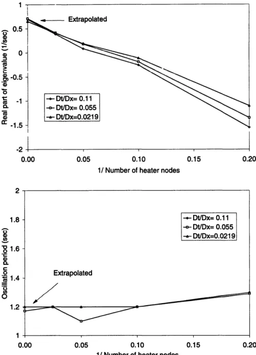
4-9 Determination of the asymptotic eigenvalue using the coupled form. . 73 4-10 Determination of the asymptotic eigenvalue using the decoupled form. 74 4-11 The measured and calculated stability boundaries. . ... 75

4-12 Schematic of fuel nodes ... .. 82

(11)

4-14 Schematic of a recirculation loop . ... . 89

4-15 Jet pump characteristics curves ... .. 97

4-16 Nodalization of the steam line system . ... 99

4-17 Turbine stop valve pressure variations in the theoretical transient .. 104

4-18 Boundary conditions for TT3 calculation . ... 105

4-19 Turbine stop valve pressures of TT3 test . ... 105

4-20 Reactor pressure controller ... 110

4-21 Recirculation flow controller ... 111

4-22 Feedwater controller ... .112

4-23 The pressure settings of the safety relief valve . ... 113

5-1 Designition of the indices of nodes and flow paths . ... . . 121

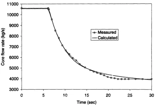
6-1 Core flow rate during Kuosheng recirculation pump trip transient. .. 145

6-2 Fission power during Kuosheng recirculation pump trip transient. .. 145

6-3 Steam dome pressure during Kuosheng recirculation pump trip transient. 146 6-4 Changes in the downcomer water level during Kuosheng recirculation pump trip transient ... 147

6-5 Steam flow rate during Kuosheng recirculation pump trip transient. . 147 6-6 Feedwater flow rate during Kuosheng recirculation pump trip transient. 148 6-7 Fission power during Peach Bottom-2 turbine trip test TT1. ... 151

6-8 Steam dome pressure during Peach Bottom-2 turbine trip test TT1.. 152

6-9 Changes in the downcomer level during Peach Bottom-2 turbine trip test TT1. ... . ... ... .. ... . .... .. 152

6-10 Fission power during Peach Bottom-2 turbine trip test TT2. ... 153

6-11 Steam dome pressure during Peach Bottom-2 turbine trip test TT2. . 153 6-12 Changes in the downcomer level during Peach Bottom-2 turbine trip test TT2. . . .. .. .. .. ... ... ... . . ... . . 154

6-13 Fission power during Peach Bottom-2 turbine trip test TT3. ... 154 6-14 Steam dome pressure during Peach Bottom-2 turbine trip test TT3. . 155

(12)

6-15 Changes in the downcomer level during Peach Bottom-2 turbine trip

test TT3 . ... ... 155

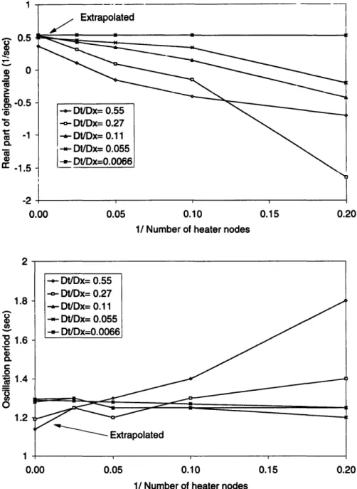
7-1 Sensitivity of time domain analysis results on the time step size and the number of axial nodes in the core channel at 63% power, 40% flow

condition. ... 160

7-2 Sensitivity of time domain analysis results on the time step size and the number of axial nodes in the core channel at 123% power, 100%

flow condition ... ... 161

7-3 Sensitivity of time domain analysis results on the void reactivity coef-ficient at 40% flow condition. ... 162 7-4 Sensitivity of time domain analysis results on the void reactivity

coef-ficient at 80% flow condition. . ... ... 163 7-5 Stability boundaries calculated by the time domain analysis procedure. 165 7-6 A segment of the Pseudo-Random Binary Sequence (PRBS). ... 166

7-7 Example of the frequency domain analysis results ... 170 7-8 Stability analysis results of test 2PT3 with different time step sizes and

core nodalization schemes . ... ... 173

7-9 Stability analysis results of test 2PT3 with different void coefficients

and time step sizes ... ... ... 174

7-10 Comparison of time domain analysis results of Peach Bottom-2 stabil-ity tests with test data ... ... 176 7-11 Comparison of stability analysis results from LAPUR-IV and the BWR

simulator with test data ... 178

7-12 Test points and stability analysis results of the Peach Bottom-2

stabil-ity tests ... ... 179

7-13 Comparison of calculated transfer function of test 2PT3 (case 1) with

the model from test data. ... ... 182

(13)

the model from test data. ... . ... 184

the model from test data. ... 185

the model from test data. ... 186

7-18 Comparison of calculated transfer function of test 3PT2 (case 2) with the model frcm test data. ... ... .... ... . 187 7-19 Comparison of calculated transfer function of test 3PT2 (case 3) with

the model from test data ... ... ... 188

the model from test data ... ... 189

B-1 Possible flow patterns of the feedwater node . ... 204 B-2 Possible flow patterns of a single-inlet, single-outlet node ... . 206 B-3 Possible flow patterns of the lower plenum with two core channels . 210 B-4 Possible flow patterns of the upper plenum with two core channels . 214

B-5 The structure of [STMA] ... . ... 227

B-6 The structure of [AM]. . ... ... 229

(14)

List of Tables

4.1 Additional relations for the steam dome model . ... . 61

4.2 Constants for decay heat calculations . ... 79

4.3 Conditions of a fuel rod transient . ... . 87

4.4 Notations used in the recirculation system model . ... 91

4.5 Conditions for theoretical steam line transient case . ... 103

5.1 The expression of Ii ... ... 131

5.2 The expression of Ffr,i ... 132

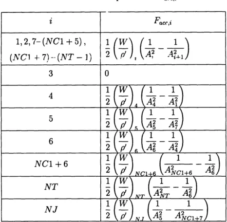
5.3 The expression of F ,,,i . ... ... ... . . 133

6.1 The specifications of Kuosheng plant . ... 143

6.2 The initial condition of the Kuosheng recirculation pump trip test . 144 6.3 The specifications of Peach Bottom-2 . ... . 149

6.4 Peach Bottom-2 turbine trip test conditions . ... 149

7.1 Frequency domain analysis results given by different weighting functions169 7.2 Test conditions and results of the Peach Bottom-2 stability tests . . . 171

7.3 Time domain analysis results of the Peach Bottom-2 stability tests 175 7.4 Parameters used in the frequency domain analysis . ... 180

7.5 Void coefficients and core nodalization schemes used in the frequency domain analysis ... .... ... 180

7.6 Frequency domain analysis results of test 2PT3 . ... 181

7.7 Frequency domain analysis results of test 3PT2 . ... 181

(15)

B.1 The elements of [AsD] for case 1 conditions. B.2 The elements of [RsD] for case 1 conditions. B.3 The elements of [AsD] for case 2 conditions . B.4 The elements of [RSD] for case 2 conditions . B.5 The elements of [AsD] for case 3 conditions . B.6 The elements of [RsD] for case 3 conditions . B.7 The elements of [AsD] for case 4 conditions . B.8 The elements of [RoSD] for uaso conditicns

B.9 The elements of [AM] . . . . B.10 The elements of [AB] ...

B.11 Non-zero elements of [AR] ...

B.12 The elements of [BR] ...

D.1 Example of SIMBA output file . . . . .

E.1 Example of POST.DAT . . . . . .

. . . . . 220 . . . . . 220 . . . . . 22 1 . . . . . 222 . . . . . 223 . . . . . 223 . . . . . 224 . . . ... 225 . . . . . . . . 228 . . . . . . . .. . 230 . . . . 232 . . . . . . . . . . . . 232 257 259

(16)

Chapter 1 Introduction

1.1 Background and Motivation

Safe and reliable operation of nuclear power reactors is the basic requirement for the utilization of nuclear energy. The stability of a nuclear power reactor with respect to internal and external disturbances must be ensured. Boiling Water Reactors (BWRs) use water both as a coolant and a neutron moderator. Bulk boiling takes place in the reactor core of a BWR. Due to the nuclear feedback and two-phase flow instability mechanisms, the possibility of BWR power oscillation exists. During the early stage of BWR development, oscillatory behaviors were observed in the BORAX reactors and the Experimental Boiling Water Reactor [1]. These reactors use natural circulation and metal fuel with low system pressure. The stability of commercial BWRs is greatly enhanced by adopting high system pressure, ceramic fuel, and core inlet orificing. Thus modern BWRs are stable at most conditions.

Nevertheless, several BWR power oscillation events have been reported in the past two decades. Following the instability event of the LaSalle County Unit 2 in 1988 [2], the search for long-term solutions to resolve the BWR stability issue began. At the same time, a set of Interim Corrective Actions was adopted by the BWR owners to minimize the possibility of instability [3]. These Interim Corrective Actions prohibit reactor operations in the regions most susceptible to power oscillations based on the past experience. However, another BWR instability event occurred in Washington

(17)

Nuclear Power Unit 2 in 1992 [4], which was operated outside the exclusion regions defined in the Interim Corrective Actions. This event shows that the unstable region depends on many factor, and is difficult to define.

After several years of research, some long-term solution options that have been proposed are approved by the U.S. Nuclear Regulatory Commission [5]. Two basic approaches are used in these long-term solution options. They are Prevention and Detection/Suppression. Automatic protection systems are required for all long-term solutions. The Prevention appcoach designates exclusion rcgions as in the Interim Corrective Actions. Operation in these exclusion regions is prevented by automatic protection systems. This approach reduces the available operation domain. Moreover, because of the complexity of the BWR instability, it is difficult to establish exclusion regions that can cover all possible operation conditions. The detection/Suppression approach uses stability monitors to detect unstable occurrences. Once detected, power oscillations are suppressed by automatic protection systems. This approach relies on the stability monitors to identify system conditions. These stability monitors must be highly reliable so that no unstable condition will be undetected, and also there shall be no false alarm.

Even if the above approaches work perfectly, they can not provide information about system stability in advance. This information will be valuable to the operators for steering the reactor out of undesirable conditions. Currently available stability monitors cannot provide stability predictions. A tool that can both detect and predict system stability margins is needed to avert unstable situations and to minimize the impact of this BWR stability issue.

1.2 Research Goals

In order to have the ability to both monitor and predict stability margins, a tool based on the deterministic approach is required. Because many system parameters affect the stability of a BWR, dynamic simulations of system parameters are necessary for accurate stability predictions [6]. Also, for a stability monitor/predictor to be useful,

(18)

its computation time must be faster or near real time. The goals of this research are

1. To develop a BWR simulator that can accurately simulate the phenomenon of power oscillations. This simulator shall be capable to simulate normal and operational transient conditions. The computation speed of this BWR simulator shall be faster than real time.

2. To develop a stability analysis procedure using this BWR simulator.

These BWR simulator and stability analysis procedure can be used for

* Stability margin monitoring and prediction,

* Operational transient analysis,

* Operator support, and

* Training.

1.3 Thesis Organization

This thesis is divided into eight chapters. Chapter 1 presents the background, moti-vation, and goals of this research. Chapter 2 gives an overview of the BWR stability issue. This chapter describes the safety concerns of BWR power oscillations, the mechanisms and modes of BWR instability, the effects of changes in system parame-ters on the stability margin, the analysis methods, and the approaches to resolve this issue.

Chapter 3 gives a brief description of modern BWRs and defines the scope of the simulation. Chapter 4 describes the physical models used in the BWR simulator. Validation results of individual models are also presented. Chapter 5 discussed the numerical solution methods for steady-state and transient calculations. Chapter 6 presents the validation results of the BWR simulator. The simulator is benchmarked

(19)

against data from the Kuosheng recirculation pump trip test and the Peach Bottom-2 turbine trip tests.

Chapter 7 describes the procedures for stability analysis in both time and fre-quency domains using this BWR simulator. The results of stability analyses of the Peach Bottom-2 stability tests using these procedures are compared to test data and the analysis results by other researchers. Chapter 8 summaries the conclusions ob-tained from this research and lists the recommendations for future research.

(20)

Chapter 2 Overview of the Boiling Water

Reactor Stability Issue

2.1 Introduction

The potential for Boiling Water Reactor (BWR) instabilities has been recognized since the beginning of BWR development. Government regulations require that a nuclear reactor be designed such that power oscillations "are not possible or can be reliably and readily detected and suppressed" [7]. For BWRs, analyses in the design stage were used to show compliance with the regulations in the past.

BWR power oscillation experience outside the United States include the Coarso in Italy [8], the Ringhals-1 in Sweden [9], and the Confrentes in Spain [10]. In the United States, two BWR power oscillation events have occurred recently. On March 9, 1988, a power oscillation event occurred at LaSalle Unit 2 (LaSalle-2) reactor [2]. This event raised concerns about the adequacy of the past analyses and the impact on plant safety; research was initiated to resolve this issue. On August 15, 1992, another power oscillation event was experienced by Washington Nuclear Power Unit 2 (WNP-2) [4]. This event again confirms the need for new approaches to ensure BWR stability.

This chapter reviews the issue of BWR stability. First, the safety concerns of BWR power oscillation are described. Then, the oscillation mechanism and the sensitivity

(21)

of stability to system parameters are discussed. Next, the methods to study BWR stability are summarized. Finally, the approaches to resolve this issue are presented.

2.2 Safety Concerns of BWR Power Oscillations

Power and flow oscillations in a nuclear reactor are very undesirable. One of the major concerns is the fuel integrity during power oscillations. If the oscillation am-plitude is large, the fuel rods may experience periodic dryout and rewetting [11]. The safety limit of the Minimum Critical Power Ratio (MCPR) may be violated during an extended period of dryout.

Another safety concern is the consequences of an Anticipated Transient Without Scram (ATWS) event. By procedure, if an ATWS event occurs the recirculation flow is reduced to reduce the reactor power. But this will drive the reactor into a high power, low flow condition which is most susceptible to power oscillations. If an ATWS event is followed by power oscillations, the heat capacity of the suppression pool may not be large enough to accommodate the possible heat load. Several analyses have shown that the mean fission power increases as the amplitude of power oscillation increases [6, 12]. The steam that is discharged into the suppression pool during the ATWS and power oscillation event may cause the temperature of the suppression pool to exceed its limit.

Because of these safety concerns, it is necessary to demonstrate the stability mar-gin of a BWR in the design stage and identify the stability boundary in the operation stage. If a power oscillation event occurs, it has to be suppressed immediately.

2.3 Mechanism of BWR Power Oscillations

The basic mechanism of BWR power oscillations has been identified as nuclear-coupled density-wave oscillations [13]. Two types of power oscillations have been observed: core-wide (or in-phase) and regional (or out-of-phase) oscillations.

(22)

2.3.1 Density-wave instability

A BWR core contains a two-phase coolant and is susceptible to two-phase flow insta-bilities. Various types of two-phase flow instabilities have been studied. At reasonably high pressures, the density-wave instability is the most commonly encountered type [14, 15, 16].

Density-wave oscillations are usually observed in systems with a two-phase mix-ture. It may also occur in a system with a single-phase fluid if the density change is large enough. The essential ingredients to produce density-wave oscillations are [17]

1. A density distribution throughout the system which depends on the flow rate of the system,

2. A time delay between the flow rate changes and the density responses,

3. A cause/effect relationship between flow rate and density changes, and pressure loss/buoyancy changes.

Density-wave instabilities can be explained by the phenomenon of kinematic wave propagation. They are caused by the finite time necessary for the enthalpy and void fraction waves to propagate in the channel. These finite propagation times induce time-lag effects and phase-angle shifts between the channel pressure drop and flow rate, which under certain conditions can result in self-sustained oscillations [14].

Consider a heated channel containing a two-phase fluid initially at steady- state. An incremental decrease in the inlet flow rate produces an increase of the void fraction along the channel. This void fraction perturbation (or density wave) travels in a speed near the vapor velocity, and produces a channel pressure drop fluctuation with a time delay with respect to the initial flow rate change. If the flow rate and pressure drop fluctuations satisfy certain relations, self-sustained oscillations may occur. The period of density-wave oscillations is usually close to twice that of the vapor transit time through the channel and is on the order of seconds [16].

Two types of density-wave instabilities have been observed: loop instabilities and parallel-channel instabilities [18]. For loop instabilities, the boundary conditions of

(23)

Out I et O0 00 0 0 O InI et TIME

Figure 2-1: Local pressure drop variations due to inlet flow fluctuation (from [19]).

the channel are determined by the flow rate versus pressure drop characteristics of the external loop. Figure 2-1 shows the variations of the local pressure gradients of a boiling channel with sinusoidal inlet flow rate fluctuations [19]. The time delay of local pressure drops introduced by the traveling density wave is shown. The resulting total channel pressure drop variation is sinusoidal but with a phase lag with respect to the inlet flow rate. If this phase lag reaches 180 degrees, then the effective channel pressure drop versus flow rate characteristic curve will have a negative slope, and loop instabilities may occur.

For parallel-channel instabilities, a constant pressure drop boundary condition is imposed by either a large number of parallel channels or a large bypass flow path. Figure 2-2 illustrates the variations of pressure drop components for parallel-channel instabilities [20]. The total pressure drop is broken down into frictional, elevation (gravity), spatial acceleration, and temporal acceleration (inertia) terms. Each term has a different dependency on velocity and void fraction profiles and, thus, has a

(24)

different phase shift with respect to the inlet mass velocity variation. Under certain conditions, the phase relationships between pressure drop components may result in a total cancellation on the pressure drop variation. Then the flow oscillations can be sustained.

Several modes of parallel-channel oscillations can occur [19]. It can be that only the flow of one channel is oscillating, while the flow of the rest of the channels stays nearly constant; or it can be that the flow of half of the channels oscillates out-of-phasc with the flow of the other half of the ohannels; or it can be three groups of channels oscillate 120 degrees out-of-phase with respect to each other.

2.3.2 Nuclear feedback

The power generation from a BWR core is coupled to the coolant thermal-hydraulic conditions through a reactivity feedback mechanism. The water in a BWR acts both as a coolant and a neutron moderator. The density of the water affects the efficiency of neutron moderation. A BWR usually has a negative void reactivity feedback coefficient. If the void fraction in a BWR core increases, it produces a negative reactivity change and the power decreases.

This coupling between the void fraction and power, combined with the dynamics of fuel rods, forms a feedback loop that can lead to power oscillations. Figure 2-3 illustrates the nuclear feedback loop in a BWR [21]. Starting from the upper left corner of Figure 2-3, an increase in voids in the core reduces reactivity and the power. The heat transfer from the fuel rods to the coolant is reduced, but with a time delay due to the thermal inertia of the fuel rods. With less heat transferred to the coolant, the void in the core is reduced, and the power is increased through the void reactivity feedback. Then, after the time delay due to fuel rod dynamics, the void is increased again. This completes a cycle of power oscillations. This mechanism when acting alone is also called reactivity instability [19].

(25)

.j w z WI_cr 4 tI•-_0; U u, _o W wJ z ~P I-. 2 0 4 hi -s hi A P 4WIC -j 6#WU

Figure 2-2: Variations of pressure drop components for parallel-channel type oscilla-tions (from [20]). Ow₀

a.

Figure 2-2: Variations of pressure drop components for parallel-channel type oscilla-tions (from [20]).

Y

(26)

Figure 2-3: Nuclear feedback loop in a BWR (adapted from [21]).

2.3.3 Modes of BWR instabilities

Three spatial modes of BWR instabilities have been observed: single channel, core-wide (in-phase), and regional (out-of-phase) oscillations [19].

Single channel oscillations were observed during special tests when a coolant chan-nel was partially blocked by a failed flowmeter. The flow of this chanchan-nel then oscillated following the density-wave mechanism while all other channels remained stable. This type of instability has been reported only once, but it can be very dangerous because it is hard to detect [19].

Core-wide oscillations are caused by loop type density-wave instabilities coupled with reactivity instabilities. In this type of instability, all the channels in the core oscillate in phase with each other. The spatial power shape during oscillations cor-responds to the fundamental mode of neutron flux shape (steady-state distribution). Axial power shape changes have also been observed during core-wide power oscil-lations. Because the whole core responds in phase, this type of oscillation can be detected by Average Power Range Monitors (APRMs).

(27)

with neutronic oscillations. During regional oscillations, part of the channels oscillate out of phase with the other channels: the power or flow of the channels in one region increases while that of the channels in the other region decreases. The power shape in regional oscillations relates to a higher harmonic mode of the neutron flux shape (subcritical modes). Normally, these subcritical modes would be damped out because the eigenvalues of these modes are less than one. However, when these subcritical flux modes are coupled with parallel-channel oscillations, sustained power oscillations can be realized [22].

The variations in the total power and flow rate during regional power oscillations are smaller than the local variations due to spatial cancellations. Multiple Local Power Range Monitors (LPRMs) are needed for early detection of out-of-phase oscillations.

2.4 Dependence of Stability on Changes in

Op-erating Variables

Many parameters affect the stability of a BWR. Because BWR power oscillations involve complex processes, the effect of a physical parameter on BWR stability some-times depends on other parameters. So it is not always possible to find a set of system parameters that can ensure stability.

In general, the following changes of individual parameter decrease stability [15, 16, 19, 21, 23, 24, 25, 26, 27]:

1. Increasing power: This increases the void content of the core, which increases feedback from the density-wave mechanism. It also increases reactivity feedback because the magnitude of the void reactivity coefficient is increased [19].

2. Decreasing core flow: This also increases the core void content.

3. Increasing two-phase pressure drop in the core: This enhances the density-wave mechanism.

(28)

4. Decreasing single-phase pressure drop in the core: This also enhances the density-wave mechanism.

5. Increasing void reactivity feedback: This enhances the reactivity feedback mech-anism.

6. Reducing the fuel rod thermal time constant: This increases the variation of heat flux on the fuel surface during power oscillations, which then increases the void fraction variations and enhances power and flow oscillations. Decreasing the fuel rod thermal time constant also reduces the phase shift between the flow rate and power responses which tends to stabilize the system. For the current BWR fuel designs, the stabilizing effect is usually out-weighed by the destabilizing effect [19, 24, 27].

7. Increasing radial peaking factor: The channel with the highest power usually has more voids and has a higher weighting for reactivity feedback. This hot channel is less stable. The stability of high power channels dominates over lower power channels. So a high radial peaking factor is destabilizing.

The effects of system pressure, axial power shape and inlet subcooling on stability are more complicated.

* System pressure: Decreasing system pressure increases the density difference be-tween water and steam, which is destabilizing. However, Blakeman and March-Leuba observed the opposite effect for extremely bottom-peaked power shapes

[23].

* Axial power shape: Bottom-peaked power shapes have a longer two-phase region and larger voids, so they are more unstable. However, extremely bottom-peaked shapes have been shown to be more stable than intermediate shapes because the reactivity weighting in the upper part is reduced [23].

* Core inlet subcooling: For the density-wave mechanism, the effect of changing inlet subcooling depends on the original inlet subcooling level [15]. At medium

(29)

or high subcoolings, an increase in subcooling increases non-boiling length and stabilizes the flow. However, at small subcoolings, the non-boiling length is very short. An increase in subcooling reduces voids near the inlet region, so the pressure drop that is in phase with the inlet flow rate is reduced, and the flow is destabilized. For nuclear feedback, increasing the core inlet subcooling reduces the void contents in the core and increases core power. The net ef-fect of increasing inlet subcooling is stabilizing when at high subcoolings and destabilizing when at low subcoolings.

Core-wide and regional oscillations have different sensitivities to system parame-ters. Regional oscillations have a large gain from parallel-channel instabilities because they do not have damping of the external loop, but they have a damped feedback from subcritical neutronic modes. The damping of subcritical neutronic modes de-pends on the eigenvalue of each mode, and a larger eigenvalue corresponds to a less damped mode. From the one-group diffusion theory, the eigenvalue of a harmonic

mode can be expressed as [28]

vEf A DB? + Ea

where

Ai is the eigenvalue of the ith neutronic mode,

vEf is the fission neutron yield times the fission cross section,

D is the diffusion coefficient,

Bi2 is the geometric buckling of the ith mode, and E, is the absorption cross section.

These eigenvalues are less than one except for the fundamental mode which is equal to one for steady-state conditions. The reactivity separation between fundamental

and subcritical modes can be expressed as [22]

1 1 DAB2

APsubcritical,i = i -- = f

(30)

where AB' = B' - B' . A small subcritical reactivity means less damping of the

subcritical mode. In that case, the reactor is more prone to the out-of-phase type instability.

So, the conditions that favor out-of-phase oscillations over the in-phase type are [19]

* low geometric buckling,

* high fission cross section,

* high pressure drop across the core,

* high core flow rate,

* high pressure loss in the external loop,

* highly bottom-peaked axial power shapes, and

* low single-phase friction.

Another important factor that greatly affects stability is the uniformity of channel hydrodynamics characteristics. If a core contains two types of channels with differ-ent pressure drop characteristics, then this core will be less stable than the cores with channels of only one type [4, 29]. Therefore, when doing reload designs, the compatibility between different fuel designs must be examined.

2.5 Analysis Methods for BWR Stability

Various methods have been used to analyze BWR stability. These methods have different applications, and they are complimentary to each other in understanding and controlling BWR stability.

BWR stability is traditionally described in terms of Decay Ratios (DRs). The decay ratio is defined as the ratio of the peak amplitude of an oscillation to that of the previous oscillation following an impulse disturbance (see Figure 2-4 [21]). A system is stable with a DR less than one, and unstable with a DR greater than one.

(31)

E Cc E a0 CO 0 0 2 4 6 Time

Figure 2-4: Definition of the Decay Ratio (adapted from [21]).

The DR relates to the poles of a system's closed loop transfer function [30]. For a second order linear dynamic system, the DR is the same for any two consecutive oscillation peaks. For higher order system, the DR is not a constant, and the appro-priate stability indicator is the asymptotic DR corresponding to the least stable poles of the system.

The decay ratio is the stability indicator for single-input, single-output systems (SISO). BWRs, however, are multiple-input, multiple-output systems (MIMO). A single DR cannot be expected to represent the whole picture of the stability of a BWR [31].

2.5.1 Experimental methods

Several BWRs have performed special stability tests [32, 33]. These tests not only determined the stability of the particular plant but also formed a data base for the qualification of analytical methods.

These tests were done by perturbing one input parameter and measuring the out-put responses of reactor power. The two inout-put parameters that have been used are

(32)

pressure and reactivity. Control rod oscillations were used to generate reactivity per-turbations. Pressure perturbations were produced by disturbing the system pressure controller.

Two time variations have been used for input perturbations. The first type is sinusoidal oscillations. Several frequencies of sinusoidal signals were used to cover the frequency range of interest. The other type of perturbation is Pseudo Random Binary Sequence (PRBS), which simulate white noise.

Collected test data were reduced by frequency domain analysis. A transfer func-tion was fitted to the test data, and the decay ratio was calculated from this transfer function.

2.5.2 Stochastic methods

Stochastic methods are based on neutron noise analysis to deduce stability informa-tion. Random processes such as the collapse of a steam bubble in the core produce noise in neutron flux signals. This noise contains information about the system.

The stability of BWRs can be estimated by methods such as an autocorrelation function, autoregressive modeling, or a power spectral density fit [30]. To have an accurate estimation, a long history of neutron noise data is needed. The required data length also depends on the system conditions: the more stable the system is, the longer data length is needed.

On-line stability monitors based on neutron noise analysis have been developed [34]. This type of stability monitor can only provide the current status. It can not predict stability that would result from changes in conditions.

2.5.3 Analytical methods

Analytical calculations of BWR stability are very complicated and require computer simulations. Many computer codes have been used to study BWR stability. They fall in two categories: frequency-domain and time-domain codes [13].

(33)

Frequency domain codes

Frequency-domain codes are developed particularly for BWR stability analysis. The procedure of stability analysis in the frequency domain is

1. Select a set of governing equations and constitutive relations,

2. Linearize these equatioiis by using a first order perturbation approximation,

3. Laplace transform the linearized equations into frequency domain, and

4. Determine the stability by using linear control theories.

The advantages of using frequency domain codes are less computer time and fewer numerical problems [29j. Some examples of frequency domain codes are FABLE, LAPUR and NUFREQ [13]. Note, however, that non-linear phenomena such as limit-cycle oscillations cannot be modeled.

Time domain codes

Time domain codes integrate the system governing equations directly, and calculate the state variables at each time step. These codes are usually general purpose codes, not developed specifically for stability analysis. They are useful in calculating system parameters, such as the peak clad temperature and MCPR during power oscillations. They can also predict the peak amplitude of non-linear limit cycle oscillations.

When using time domain codes to study BWR stability, special caution should be paid to the numerical damping problem [6]. Many time domain codes incorporate special numerical methods for avoiding numerical instability and reducing computer time. Numerical schemes such as up-wind differencing and multi-step methods will produce a numerical damping effect that may mask the oscillatory behavior.

Examples of time domain codes used for BWR stability analysis are RAMONA-3B, TRAC-BF1, TRACG, RETRAN, BNL EPA, SABRE, TRAB, TOSDYN-2, STANDY, and SPDA [13].

(34)

2.6 Approaches for Resolution of the BWR

Sta-bility Issue

2.6.1 Interim Corrective Actions

After the LaSalle-2 event, a set of Interim Corrective Actions were adopted by the BWR owners while the research for long term solutions was ongoing [3]. The Interim

Corrective Actions define exclusion regions on the power-flow map (see Figure 2-5). These high power, low flow regions are most susceptible to instability. In these regions, the natural circulation flow contributes to a large portion of the total core flow. So the core flow is very sensitive to the void contents in the core. This situation enhances the density-wave instability.

Region A in Figure 2-5 is the area above 100% rod line and on the left of the 40% flow line; Region B is the area between 100% and 80% rod lines, and on the left of the 40% flow line; Region C is the area above 80% rod line and on the left of the 45% flow line. Operation within Regions A and B are prohibited, and if entered, the operators should bring the reactor out of these regions immediately by inserting control rods or scram. Operation in Region C is allowed only for control rod with-drawals during startup requiring Preconditioned Interim Operational Management Recommendations (PCIOMR). Operators are also required to scram the reactor if power oscillations occur, or if all the recirculation pumps are tripped.

The operating point of the WNP-2 when power oscillations occurred is outside the exclusion regions. This event proves again that the approaches used in the past are insufficient in dealing with BWR stability problem. It also shows that these exclusion regions do not cover all the unstable conditions.

2.6.2 Long Term Solutions

Before the LaSalle-2 event occurred, it was believed that an analysis is sufficient to ensure compliance with regulatory requirements on BWR stability. Now, an auto-matic protection system is required for resolving the stability issue. The Boiling

(35)

100 " 80 o60-o 40-a. 20 - 0-0 20 40 60 80 100 120

Core flow (% of rated)

Figure 2-5: Exclusion regions defined by the Interim Corrective Actions (adapted from [3]).

Water Reactor Owners' Group (BWROG) has developed several options for the long term solution, and the U.S. Nuclear Regulatory Commission (NRC) has accepted some of the options [2, 5]. The proposed Long Term Solutions are based on two basic approaches:

1. Prevention-regional exclusion with automatic protection actions, and

2. Detection and Suppression.

The automatic protection actions being considered are reactor scram and selected rod insertion (SRI). The prevention approach is basically the same as the Interim Corrective Action except that operation in the exclusion regions is prevented by an automatic protection system instead of administrative control. This approach requires minimum plant modifications, but reduces the available operation domain. To define a conservative exclusion region for a wide range of operating conditions is the biggest challenge for adopting this approach.

The second approach uses LPRM based stability monitors such as Oscillation Power Range Monitors (OPRMs) to detect power oscillations. This approach does not

Extended load line

0% rod line 80% rod line

control lines

Natural circulation line Minimum power line

(36)

impose any restriction on the operation domain. The reliability of stability monitors is the main concern for this approach.

2.6.3 Stability control

Controlling BWR stability during normal operation is not straightforward because many factors affect stability. An operational strategy has been proposed for main-taining large stability margins [35]. This control strategy is to maintain the average bulk boiling boundary above a predetermined alevation. With a sufficient length of the single-phase region, density-wave oscillations are suppressed, and the stability can be ensured.

The location of the average bulk boiling boundary depends on many parameters that are also important to stability, such as pressure, power, core flow rate, inlet subcooling and core power distribution. Changes in these parameters will be reflected in the change in the location of the boiling boundary. It has been shown that the stability margin of the system is insensitive to changes in operating parameters as

long as the average bulk boiling boundary is above a predetermined height.

The desired boiling boundary height is not always achievable, however. The achievable power shapes are limited by fuel loading, burnup, and other safety lim-its. The boiling boundary control strategy may be in conflict with other operating recommendations.

2.7 Chapter Summary

Recent BWR power oscillation events have prompted the need for new approaches to ensure BWR stability. Two major concerns are the thermal margin of the fuel during power oscillations, and the possible consequences of an ATWS plus power oscillation event.

The mechanism of BWR power oscillations is nuclear-coupled density-wave insta-bility. Many parameters affect BWR stability, and their effects on stability are some-times counter intuitive. BWR stability can be analyzed by experimental, stochastic,

(37)

or analytical methods. However, because of the complexity of the processes, it is dif-ficult to establish a stability boundary that could cover all the operation conditions.

Two basic approaches have been proposed for the long term solution: Prevention, and Detection/Suppression. An operational strategy that controls the core average boiling boundary elevation has also been proposed for maintaining a large stability margin. These approaches either restrict the operation domain or impose risk from inadvertent actuation of the safety system.

.A simulator -based stability monitor/predictor can alleviate the side effects of the long term solutions. The capability of both monitoring and predicting stability mar-gin makes the simulator-based stability monitor more useful than a stochastic-based stability monitor. With a simulator-based stability monitor/predictor, the opera-tors can keep track of the current stability margin as well as the stability conditions at future operating points. Thus unnecessary challenge to the automatic stability protection system can be avoided.

(38)

Chapter 3 BWR Simulator

-

Overview

3.1 Description of a BWR

Modern BWR power plants employ a direct steam cycle as shown in Figure 3-1 [36]. This system consists of a BWR Nuclear Steam Supply System (NSSS) and a con-ventional Balance-of-Plant (BOP). The steam generated in the reactor vessel goes directly into the main turbine. After expansion through turbine stages, the exhaust steam is condensed into water in the main condenser. The condensed water is puri-fied, heated up, and pressurized by the condensate and feedwater systems, and is fed into the reactor vessel as the feedwater.

The reactor vessel of a BWR is an integrated steam generating unit. It encloses the nuclear reactor core, steam separators, and steam dryers. Figure 3-2 [37] shows the steam and recirculation water flow paths in a BWR of General Electric (GE) design. The single-phase coolant flows up into the reactor core by forced circulation. In the reactor core, the coolant is heated up by the nuclear fission power, and is turned into a two-phase mixture. The coolant then exits the reactor core, flows through the upper plenum and stand pipes, and enters the steam separators. The steam in the two-phase mixture is separated out and dried by the steam separators and dryers, and exits the reactor vessel to the main steam lines.

The water separated from the steam goes down to a water pool surrounding the separators, and flows into the downcomer between the reactor vessel and core shroud.

(39)

c

u

LI U w U) LI

(40)

Figure 3-2: Steam and recirculation flow paths (from [37]).

The feedwater flow is sprayed down through the feedwater spargers into the down-comer and mixes with the returning liquid flow from the separators and dryers. Part of this mixed flow of water leaves the reactor vessel to the recirculation system, is pressurized by the recirculation pumps, re-enters the reactor vessel and is injected into the jet pumps with high velocity through the jet pump nozzles. The rest of the mixed flow is sucked into the jet pumps by the low pressure created by the high speed jet stream. The combined flow is discharged into the lower plenum through the jet pump diffusers. This recirculation and jet pump system provides the pressure head for the forced circulation of the coolant through the core. An alternative to the jet pump system for driving core flow is the use of internal recirculation pumps.

The reactor power level is controlled mainly by two systems. The first one is the control rod system. BWRs employ bottom entry control rods. The control rods are used for three purposes:

(41)

2. To adjust the power distribution shape;

3. To provide a large amount of negative reactivity for reactor scram.

The second system that controls the power is the recirculation system. Changes in the recirculation flow affect the flow through the core and the amount of vapor in the core. Because of the negative void reactivity coefficient, the reactor power is changed in the opposite direction as the core vapor content. By changing the recirculation flow, the reactor power can be adjusted _'2 st and uniformly.

The 100% and 80% rod lines shown in Figure 2-5 (page 35) are typical BWR flow control lines. Operation along these forced convection flow control lines can be achieved without control rod movement. Power changes of up to 25% of rated power can be accomplished automatically by the recirculation flow control system

[38]. The changes in the recirculation flow are controlled by using either variable-speed recirculation pumps or flow control valves.

3.2 Scope of the Simulation

The main focus of this BWR simulator is to simulate the phenomenon of BWR power oscillations accurately. Thus the scope of the simulation is limited to the portion of a BWR that is related to the processes of power oscillations. The simulator developed here covers the major components inside the reactor vessel, the external recirculation system, and the main steam system including the turbine bypass lines.

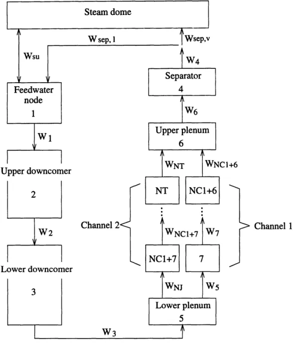
The nodalization of this BWR simulator is shown in Figure 3-3. Except for the steam dome node, all the nodes have constant cross sectional areas. The steam dome node represents the vapor space and the water pool outside the steam dryers and separators. The feedwater mixing node is used to model the part of downcomer that contains the feedwater spargers. The upper downcomer node is the part of downcomer below the feedwater mixing node and above the jet pumps. The lower downcomer node covers the jet pumps and the external recirculation lines. Two separate recirculation loop models are used to calculate the pressure difference and

(42)

flow rate across the lower downcomer node. Each recirculation loop model consists of one recirculation pump, one flow control valve, and one jet pump. The lower plenum, upper plenum, and the dryer/separator are each represented by one node. The standpipes are included in the dryer/separator node.

The reactor core region is the only region with flexibility in nodalization. The core can be modeled by either a single channel or two parallel channels connected only at plena. The core channels are formed by axial stacks of fuel nodes. The total number of core nodes is limited to 40. Within each fuel nole, the radial temperature distribution of the fuel rods and the heat flux to the coolant are calculated by a fuel conduction and convection model. This flexible scheme of modeling the core allows for many simulation choices. The reactor core can be represented by a single channel, or one core channel with one bypass channel, or two core channels with each representing a half of the core.

The main steam lines are modeled by a single string of nodes. Two nodes are used to represent the steam lines inside the containment upstream of the Main Steam Isolation Valves (MSIVs). Four nodes are used for the steam line between the MSIVs and the turbine stop/control valves. The turbine bypass lines are modeled by one node. The safety/relief valves, the MSIVs, the turbine stop/control valves, and the turbine bypass valves are each simulated by one valve.

The boundary points of the simulator are upstream of the feedwater nozzle, and downstream of the safety valve, turbine control valve, and turbine bypass valve. The flow rate of the feedwater is calculated by the feedwater controller. The feedwater enthalpy is specified as an input parameter, and can be varied with time. The pressure at the downstream of the safety valve is fixed at the suppression pool pressure. The pressure at the turbine bypass valve outlet is at the main condenser pressure. The pressure after the turbine control valve is also fixed and is specified as an input parameter.

The BWR simulator developed here is simple when compared to other system codes. However, it is versatile and has enough details for simulations of many opera-tional transient events.

(43)

0 co c>

ee

Li

H a0

Li

LiQ

0 N 0d

z

(44)

3.3 Chapter Summary

Modern BWR power plants use a direct steam cycle consisting of a BWR nuclear reactor and a conventional steam plant. The power level of a BWR is controlled by control rods and the recirculation flow rate. In this research, the major components in the reactor vessel, the recirculation system, and the main steam lines are covered in the BWR simulator. The BWR is modeled by nodes of constant cross sectional area, except for the steam dome node. The core region can be modeled flexibly to accommodate different simulation needs. This BWR simulator is simple, yet it also has enough details to simulate operational transient conditions.

(45)

Chapter 4 Development of Models of

Physical Processes

The physical processes involved in a BWR include single- and two-phase fluid flows, conductive and convective heat transfer, nuclear fission and decay power generation, and control actions. Because the aim of this research is to develop a fast-running BWR simulator, the physical processes are modeled with simplifications. Nevertheless, these models are capable of simulating BWR power oscillations accurately.

The BWR simulator consists of six main modules:

1. Thermal-hydraulic model;

2. Core neutronics model;

3. Fuel conduction and convection model;

4. Recirculation system and jet pump model;

5. Steam line model;

6. Control system model.

The details of these models are discussed below. The results of validation calcu-lations for individual models are also presented.

A boiling water reactor simulator for stability analysis

A Boiling Water Reactor Simulator for Stability

Analysis

by

Chi Kao

Doctor of Philosophy

APR

2 2 1996

A Boiling Water Reactor Simulator for Stability Analysis

by

Chi Kao

Abstract

Acknowledgments

Contents

___

List of Figures

List of Tables

Chapter 1

Introduction

1.1

Background and Motivation

1.2

Research Goals

1.3

Thesis Organization

Chapter 2

Overview of the Boiling Water

Reactor Stability Issue

2.1

Introduction

2.2

Safety Concerns of BWR Power Oscillations

2.3

Mechanism of BWR Power Oscillations

2.3.1

Density-wave instability

2.3.2

Nuclear feedback

2.3.3

Modes of BWR instabilities

2.4 Dependence of Stability on Changes in

Op-erating Variables

[23].

2.5

Analysis Methods for BWR Stability

2.5.1

Experimental methods

2.5.2

Stochastic methods

2.5.3

Analytical methods

2.6

Approaches for Resolution of the BWR

Sta-bility Issue

2.6.1

Interim Corrective Actions

2.6.2

Long Term Solutions

2.6.3

Stability control

2.7

Chapter Summary

Chapter 3

BWR Simulator

-

Overview

3.1

Description of a BWR

c

u

3.2

Scope of the Simulation

ee

Li

Li

LiQ

z

3.3

Chapter Summary

Chapter 4

_{2 2 1996}