Automatic 3D surface area measurement for vitiligo lesions

Automatic 3D Surface Area Measurement for

Vitiligo Lesions

by

Jiarui Huang

Submitted to the Department of Electrical Engineering and Computer

Science

in partial fulfillment of the requirements for the degree of

Master of Engineering in Electrical Engineering and Computer Science

at the

MASSACHUSETTS INSTITUTE OF TECHNOLOGY

June 2017

c

○ Massachusetts Institute of Technology 2017. All rights reserved.

Author . . . .

Department of Electrical Engineering and Computer Science

May 30, 2017

Certified by . . . .

Anantha Chandrakasan

Vannevar Bush Professor of Electrical Engineering and Computer

Science

Thesis Supervisor

Accepted by . . . .

Christopher J. Terman

Chairman, Masters of Engineering Thesis Committee

Automatic 3D Surface Area Measurement for Vitiligo Lesions

by

Jiarui Huang

Submitted to the Department of Electrical Engineering and Computer Science on May 30, 2017, in partial fulfillment of the

requirements for the degree of

Master of Engineering in Electrical Engineering and Computer Science

Abstract

Vitiligo is a long term skin depigmentation disease that may result in psychologi-cal stress. Monitoring changes in vitiligo lesion area allows assessment of treatment efficacy and aids in clinical decision making. Currently existing approaches for vi-tiligo lesion measurement are either inefficient or inaccurate. Using a RGB-D camera (Kinect) and imaging processing techniques, we develop an automated skin lesion screening system (VLAMS) that can be widely adopted in clinics. VLAMS is tested using clinical medical data. Results show VLAMS can consistently segment target lesion region and accurately measure lesion area of any skin surface.

Thesis Supervisor: Anantha Chandrakasan

Acknowledgments

This thesis would not have been where it is today if not for the help and guidance of a number of essential people. First of all, I would like to thank my thesis advisor, Professor Anantha Chandrakasan, for allowing me to join his group and work on this interesting research. It has been a great experience working at MTL. Secondly, I would like to thank Dr. Victor Huang. This project would not have been initiated without him identifying the clinical problem and importance of a 3D based solution. He provided a lot of help with IRB application as well as coordinated the data collection at the clinics. Thirdly, I would like to thank Priyanka Raina. She not only provided invaluable help and guidance in this project but also has given me positive influence in academics. I have learned a lot from her. Finally, I would like to thank my parents, my grandma and all my friends for their support in my entire life. Their love has been my biggest motivation.

Contents

1 Introduction 15

1.1 Motivation . . . 15

1.2 Related Work . . . 16

1.2.1 3D Reconstruction . . . 16

1.2.2 The Visitrak System . . . 16

1.2.3 Image J . . . 17

1.2.4 Computer-based Image Analysis Program . . . 17

1.3 IRB Approval . . . 19

1.4 Thesis Outline . . . 20

2 System Overview 21 2.1 Technical Terms . . . 21

2.1.1 Kinect . . . 21

2.1.2 Depth Image and RGB Image . . . 22

2.1.3 Planimetry Measurement and Visitrak . . . 22

2.2 System Workflow . . . 23

3 Hardware Components 25 3.1 Depth Parameters Calibration . . . 25

3.2 Coordinate Mapping . . . 27

4 Software Components 31 4.1 Image Alignment and Registration . . . 31

4.2 Contrast Enhancement . . . 32

4.2.1 Gamma Correction . . . 32

4.2.2 Histogram Equalization . . . 32

4.2.3 CLAHE . . . 35

4.2.4 Lab Color Space . . . 36

4.2.5 Integrated Tool . . . 37 4.3 Lesion Segmentation . . . 38 4.3.1 Grabcut . . . 38 4.3.2 Watershed . . . 39 4.4 Area Calculation . . . 42 5 Performance 47 5.1 Test Data . . . 47 5.1.1 Area Calculation . . . 47 5.1.2 Lesion Segmentation . . . 49 5.2 Medical Data . . . 53 6 Conclusion 59 6.1 Contribution . . . 59 6.2 Challenges . . . 60 6.3 Future Work . . . 60

6.3.1 Better Camera with Higher Resolution . . . 60

6.3.2 Depth Frame Reconstruction . . . 61

6.3.3 Additional Lighting Option . . . 62

List of Figures

1-1 A typical vitiligo lesion on the eye [1]. . . 15 1-2 Example of using the Visitrak system to measure a lesion: (a) manually

tracing the lesion outline, (b) grid sheet is retraced on digital pad to calculate area [4]. . . 17 1-3 An example of using Image J for wound measurement. The white

sticker is placed next to the wound for calibration [7]. . . 18 1-4 Measured area of the same wound photographed from different angles

using Image J. The error caused by the angle can be as large as 41.366% [8]. . . 18 1-5 [9] fails to determine the right region when the lesion boundary is not

well defined. . . 19

2-1 Two generations of Kinect. Kinect V1 is shown on the left and Kinect V2 on the right [10]. . . 22 2-2 Workflow of VLAMS. Hardware dependent process is marked in grey

and software dependent process marked in white. The final result is kept for each individual patient. . . 24

3-1 The set-up for calibrating depth parameters. A ruler is used to locate the test object (green). . . 26 3-2 Calibration of parameters for Kinect V1. Data points are marked in

3-3 Images captured by Kinect V2: (a) RGB image (1920×1080), (b) depth image (512 × 424). Dimensions of two images are different. Black area indicates missing depth values. . . 29 3-5 Zoom-in comparison between the original depth image (a) and the

smoothed depth image (b). The black pixels that indicate no depth values in (a) diminish in (b). . . 29 3-4 Coordinate mapper maps RGB image onto depth image: (a) mapped

depth image, (b) overlaid image. The black spherical lines are due to different resolutions. The two black strips at both sides are due to differences of field of views. The black triangular region of the lower right corner is due to non-measurable depth and environment interference. . . 30

4-1 Gamma correction with no amplification and shift (𝛼 = 1.0, 𝛽 = 1.0). Notice that 𝛾 = 1.0 represents the original image. . . 33 4-2 Image before and after histogram equalization with corresponding

his-togram. In the original image, histogram skews to the right, which in-dicates a potential of over exposure. By equalizing histogram, a more evenly distributed histogram is achieved. More details in the shadow and the highlight are now visible in the image. . . 34 4-3 Contrast limitation is applied to avoid amplifying noise. Values that

are beyond threshold 𝛽 in (a) are clipped and distributed in (b) [16]. 35 4-4 Images with their corresponding histograms underneath. The original

image focuses on artistic expression while details are ignored. On the right, the chair is not recognizable in the original image. After his-togram equalization, the chair is more visible but the details on the canvas are lost. By applying CLAHE, chair becomes more visible and details on the canvas are preserved. The difference can also be inferred from the changes in the histogram. CLAHE shapes the histogram more evenly and smoothly than normal equalization. . . 36

4-5 RGB image converted into Lab color space. L channel stores the light-ness information while a and b channels store color information. . . 37

4-6 An example of processing a vitiligo lesion image using contrast en-hancer. The original image is on the left and enhanced image on the right. After applying CLAHE in Lab color space and with some gamma correction, more hidden vitiligo lesions become apparent. Notice on the upper left corner, lesions are barely noticeable in the original image. The ranges for 𝛼, 𝛽 and 𝛾 are 0 − 3, 0 − 100 and 0 − 3 respectively. 38

4-7 A3 paper segmentation using grabcut algorithm. (a) The original RGB image. (b) A rectangle box is drawn to bound the object for segmen-tation. (c) Markers of different colors used to indicate background and foreground. (d) Final output. . . 40

4-8 Comparison between Grabcut and Watershed on multiple lesions. (a) The original RGB image. (b) Image after contrast enhancement. (c) Grabcut segmentation based on the contrast-enhanced image. (d) Wa-tershed segmentation based on the contrast-enhanced image. (e) Grab-cut segmentation based on the original image. (f) Watershed segmen-tation based on the original image. (g) The ground truth. . . 42

4-9 If area is directly calculated from the RGB image without depth infor-mation, the area of projection 𝑇 instead of the actual surface area 𝑆 (dark grey) is obtained [21]. . . 43

4-10 One single pixel captures a projected area ∆𝑆 at distance 𝐷. . . 44

4-11 Example of using central difference to approximate gradient. Three pixels (𝑖−1, 𝑗), (𝑖, 𝑗), and (𝑖+1, 𝑗) correspond to three physical location 𝑥 − 𝑡, 𝑥 and 𝑥 + 𝑡. The gradient (green) at point (𝑥, 𝐿(𝑥)) is approxi-mated by the slope (red) of the line connecting point (𝑥 − 𝑡, 𝐿(𝑥 − 𝑡)) and point (𝑥 + 𝑡, 𝐿(𝑥 + 𝑡)). . . 45

5-1 Measurement of a box with known surface area at 914 mm (approxi-mately 3 ft). Image taken by Kinect V2. The ruler on the floor helps locate the distance. (a) The RGB image. (b) Overlaid with mapped depth image. (c) Segmentation result. . . 48 5-2 Measurement error at different distance. . . 49 5-3 Lesion segmentation comparison. (a) The original image. (b) The

ground truth. (c) Result from VLAMS. (c) Results from [9]. . . 50 5-4 Lesion segmentation comparison. (a) The original image. (b) The

ground truth. (c) Result from VLAMS. (c) Results from [9]. . . 51 5-5 Lesion segmentation comparison. (a) The original image. (b) The

ground truth. (c) Result from VLAMS. (c) Results from [9]. . . 52 5-6 Lesion segmentation: (a) original RGB image, (b) segmentation on

enhanced image, (c) segmentation on original image. . . 54 5-7 Lesion comparison: (a) lesion in the image, (b) tracing on cellophane. 55 5-8 Lesion segmentation: (a) original RGB image, (b)segmentation on

orig-inal image. . . 56 5-9 Lesion comparison: (a) lesion in the image, (b) tracing on cellophane.

The tracings are drawn on a curved surface, and when flattened on cellophane, they appear differently from the image. . . 56 5-10 Lesion segmentation: (a) original RGB image, (b) segmentation on

enhanced image, (c) segmentation on original image. . . 57 5-11 Lesion comparison: (a) lesion in the image, (b) tracing on cellophane. 58

6-1 Cameras with different resolution: (a) camera with a low resolution can only sample 4 points on a curved surface, (b) camera with a high resolution can sample 9 points. . . 61

List of Tables

3.1 Multiple measurements correspond to different points on the object at

the same depth. . . 26

4.1 Comparison between two segmentation algorithms based on the contrast-enhanced image and the original image. . . 42

5.1 Area measurement at different distances. . . 48

5.2 Segmentation accuracy comparison between two systems. . . 50

5.3 Segmentation accuracy comparison between two systems. . . 51

5.4 Segmentation accuracy comparison between two systems. . . 52

5.5 Area measurement comparison. . . 55

5.6 Area measurement comparison. . . 56

Chapter 1

Introduction

1.1

Motivation

Vitiligo is a long-term skin condition characterized by patches of skin losing their pigment. The patches of affected skin become white and usually have sharp margins. Vitiligo affects people with all skin types, but is most noticeable in those with dark skin. Figure 1-1 shows a typical vitiligo lesion on the eye.

Figure 1-1: A typical vitiligo lesion on the eye [1].

Vitiligo is not life-threatening nor contagious. However, because patients affected with vitiligo can have areas of depigmentation anywhere on the body including face,

eyes and even inside the mouth, the undesirable depigmentation can cause long-term psychological discomfort and has a negative impact on the patient’s quality of life. There is currently no cure for this disease and the most efficient treatment shows slow progress. Moreover, current treatment progress estimated based on visual observation could be very inaccurate and misleading.

In this thesis, we develop VLAMS (Vitiligo Lesion Area Measurement System) which aims to give a quantified measurement of vitiligo lesions using a depth plus color image capture system and image processing techniques. By providing an accurate measurement of lesion areas, we hope VLAMS can be adopted in clinics to provide a visualization of the treatment progress and a measure of the treatment efficacy and thus motivate vitiligo patients to constantly receive treatment.

1.2

Related Work

1.2.1

3D Reconstruction

Three dimensional (3D) image reconstruction [2] is a procedure of creating a 3D model of the target object. One approach to measure lesion area is to use the 3D imaging technique to create a 3D model of the lesion. Unfortunately, the state-of-art 3D reconstruction process is computationally expensive and requires precise calibration and mathematical approximation, thereby making it impractical for routine clinical assessment of lesion area.

1.2.2

The Visitrak System

The Visitrak system [3] (Smith NephewWound Management, Inc, Largo, Florida) is a digital planimetry lesion measurement system. The lesion is manually traced onto a Visitrak grid sheet, which is then retraced onto the Visitrak pad that automatically completes the area calculations. The Visitrak system is easy to use but the tracing takes time because of the complex shape of the lesion. Also, it may cause discomfort

to the patient while the doctor is tracing the lesion. The use of the Visitrak system is shown in Figure 1-2.

(a) (b)

Figure 1-2: Example of using the Visitrak system to measure a lesion: (a) manually tracing the lesion outline, (b) grid sheet is retraced on digital pad to calculate area [4].

1.2.3

Image J

Image J is an open-source, Java-based image processing program developed at and distributed by the National Institutes of Health [5] [6]. To use Image J to measure a lesion, the lesion needs to be photographed first with a ruler in the photographic frame to allow Image J calibration, as shown in Figure 1-3. The lesion outline needs to be manually traced and then the Image J software can calculate the lesion area using trigonometry. Compared to Visitrak, this method is non-lesion-contact but it has low accuracy.

1.2.4

Computer-based Image Analysis Program

In [9], an image analysis program for vitiligo lesions is developed and tested on data from 10 vitiligo patients. It uses scale invariant feature transform based feature matching approach to transform and align identified lesions from follow-up images with those in the initial images. Then, the automated program detects differences

Figure 1-3: An example of using Image J for wound measurement. The white sticker is placed next to the wound for calibration [7].

in lesion area and traces the differences to examine whether the repigmentation has increased or decreased. However, this system fails at assessing large lesions and gives inaccurate measurement over curved surfaces, as shown in Figure 1-5. In addition, this technique only gives a relative change in area, rather than an absolute value for area, which makes comparing different lesions for the same person or across different people impossible.

Figure 1-4: Measured area of the same wound photographed from different angles using Image J. The error caused by the angle can be as large as 41.366% [8].

All the aforementioned approaches have drawbacks and shortcomings. These prob-lems are addressed by VLAMS. VLAMS is user-friendly, non-lesion-contact and able to give absolute measurement of lesion area over any surface.

Figure 1-5: [9] fails to determine the right region when the lesion boundary is not well defined.

1.3

IRB Approval

We work with Dr. Victor Huang at Brigham and Women’s Hospital/Faulkner for clinical assessment of VLAMS. We completed and submitted the Harvard Affiliated Application for Institutional Review Board (IRB) Review of Multi-Site Research. Our application has been successfully reviewed and accepted (Federal Wide Assurance: FWA00004881 and FWA00000484).

1.4

Thesis Outline

In this thesis, we describe the design and implementation of VLAMS, which auto-mates the vitiligo lesion measurement. We evaluate VLAMS by using test data and clinical data.

In Chapter 2, we describe the fundamentals and the workflow of VLAMS. We also present the design idea.

In Chapter 3, we describe the hardware components including calibration and de-velopment.

In Chapter 4, we describe the software components. We also discuss the algo-rithms that VLAMS uses.

In Chapter 5, we evaluate the performance of VLAMS on test data and clinical data, and compare the results with [9].

Finally, in Chapter 6, we present an overall summary of the performance of VLAMS and its contribution to the field. We also discuss potential improvements.

Chapter 2

System Overview

VLAMS uses imaging techniques for lesion area measurement. It consists of two main components: a hardware dependent component and a software dependent component. VLAMS is designed such that it is easy to maintain and upgrade. The protocol for data transmission between the hardware and software components is simple; the hardware outputs image information and specifications and the software parses this data and processes it. This independence allows future upgrades of the software or hardware components. For example, if a better camera with higher resolution is used for data collection, it will not affect the software processing. We will elaborate on the structure and workflow of the system in the following sections.

2.1

Technical Terms

The comprehension of a few terms is essential to the understanding of this thesis.

2.1.1

Kinect

VLAMS uses Kinect as its main data collector. Kinect is a motion sensing input device by Microsoft for Xbox 360, Xbox One video game consoles and Microsoft Windows PCs. Kinect has built-in color and infrared cameras, which enable a user to capture depth and color images at the same time. In this thesis, we make use of

Kinect’s depth detection capability to capture raw data. We refer to the first version of Kinect, specifically model 1517, as Kinect V1 and the second version of Kinect, which is also called Kinect for XBox One, as Kinect V2.

The major differences between these two generations of Kinects are image reso-lutions and sensing techniques. Kinect V1 has a color image resolution of 640 × 480 pixels and a depth image resolution of 320 × 240 pixels while Kinect V2 has a color image resolution of 1920 × 1080 pixels and a depth image resolution of 512 × 424 pixels. Kinect V1 uses stereopsis while Kinect V2 uses time-of-flight for depth mea-surement. Because of the different techniques used to measure depth, the effective depth measurement ranges are also different. Kinect V1 has an effective measurement range from 0.4 𝑚 to 4 𝑚 while Kinect V2 has a range from 0.5 𝑚 to 4.5 𝑚.

Figure 2-1: Two generations of Kinect. Kinect V1 is shown on the left and Kinect V2 on the right [10].

2.1.2

Depth Image and RGB Image

A depth image is a special kind of image in which each pixel represents the distance of the object in the pixel from the camera. An RGB image is an ordinary image with a vector of three values stored in each pixel. These three values represent the intensity of each color. For example, a pixel with color tuple of [255, 0, 0] is red and a pixel with color tuple of [0, 0, 0] is black.

2.1.3

Planimetry Measurement and Visitrak

Planimetry measurement [11] is one of the widely-used area measurement techniques and is used at Brigham and Women’s Hospital/Faulkner for vitiligo area measure-ment. A doctor places a piece of transparent cellophane on top of the lesion region

and uses a marker to trace the lesion boundary. After that, a planimetry device will use the tracing on the cellophane to calculate the lesion area. This manual tracing method is used as a baseline to validate the accuracy of VLAMS.

2.2

System Workflow

1. Camera captures an RGB image and stores the corresponding depth information in a separate file. These raw data files are labeled with the patient’s number and date.

2. VLAMS parses the RGB and depth data files, and registers both data files.

3. VLAMS pre-processes the RGB image using a contrast enhancement tool.

4. The contrast-enhanced RGB shows a more distinguishable contour and is used for lesion segmentation.

5. Segmented lesion area is calculated using depth data.

Figure 2-2: Workflow of VLAMS. Hardware dependent process is marked in grey and software dependent process marked in white. The final result is kept for each individual patient.

Chapter 3

Hardware Components

In this chapter, we discuss the calibration of Kinect for later experiments. Calibration includes raw depth value conversion and coordinate mapping, which are crucial for area measurement.

3.1

Depth Parameters Calibration

Unlike Kinect V2, which gives depth values directly, Kinect V1 returns raw depth data from its depth sensor. In order to proceed with area calculation, we need to convert the raw depth data into depth values in millimeters. The raw depth data from the kinect are not linearly proportional to physical depth. Instead, they follow the following formula:

𝐷(𝛼, 𝛽) = 1 𝛼𝑅 + 𝛽

where 𝐷 is the depth in millimeters, 𝑅 is the raw depth and 𝛼 and 𝛽 are the intrinsic parameters associated with the sensor.

The strategy to evaluate 𝛼 and 𝛽 is to collect a data set of readout 𝑅 and actual depth value 𝐷 by placing a test object at different known distances, as shown in Fig-ure 3-1. Then, we run nonlinear regression on this data set to minimize a predefined error function.

Reference Depth Raw Depth Value 2 ft 511, 508, 512, 511 2 ft 6 inches 629, 629, 631, 631 3 ft 707, 706, 709, 705 3 ft 6 inches 762, 762, 760, 762 4 ft 804, 805, 805, 804 4 ft 6 inches 833, 834, 834, 834

Table 3.1: Multiple measurements correspond to different points on the object at the same depth.

Figure 3-1: The set-up for calibrating depth parameters. A ruler is used to locate the test object (green).

In order to minimize the expected measurement error at different distances, define the squared error function to be:

𝜀(𝛼, 𝛽) =∑︁(𝐷(𝛼, 𝛽) − ˆ𝐷)2

where 𝐷 is the measured depth and ˆ𝐷 is the reference depth. For this nonlinear equation, we can find the optimal parameters mathematically by solving the equations obtained by setting the derivatives to zero:

𝜕𝜀 𝜕𝛼 =

∑︁𝜕(𝐷 − ˆ𝐷)2 𝜕𝛼 = 0

𝜕𝜀 𝜕𝛽 =

∑︁𝜕(𝐷 − ˆ𝐷)2 𝜕𝛽 = 0

However, this approach is tedious and error-prone. Instead, we use gradient descent to efficiently calculate the parameters:

𝛼𝑛+1 = 𝛼𝑛− 𝜂𝜕𝜀 𝜕𝛼(𝛼 𝑛 , 𝛽𝑛) 𝛽𝑛+1 = 𝛽𝑛− 𝜂𝜕𝜀 𝜕𝛽(𝛼 𝑛_{, 𝛽}𝑛₎

where 𝜂 is the step size for updating the parameters and the gradient can be calculated by using central difference approximation:

𝜕𝜀 𝜕𝛼 ≈ 𝜀(𝛼 + 𝛿, 𝛽) − 𝜀(𝛼 − 𝛿, 𝛽) 2𝛿 𝜕𝜀 𝜕𝛽 ≈ 𝜀(𝛼, 𝛽 + 𝛿) − 𝜀(𝛼, 𝛽 − 𝛿) 2𝛿

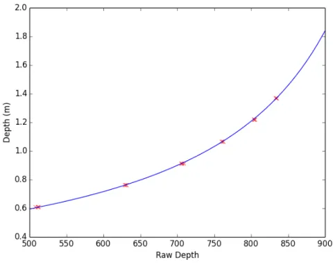
We first collect a data set of raw depth values and their corresponding depth, shown in Table 3.1. After 106 _{iterations of gradient descent, we obtain an optimal}

𝛼 = −0.0028400 and 𝛽 = 3.0996735, and we use these two values for later experiments and research. Nonlinear regression result is plotted in Figure 3-2.

3.2

Coordinate Mapping

In order to calculate the surface area, we need to register the depth image on top of the RGB image. Unfortunately, the RGB image and the depth image are captured by different cameras in Kinect and have different resolutions. Simply scaling them and stacking one on top of the other does not give desirable results. The difference in dimension is shown in Figure 3-3.

For this reason, we need coordinate mapper [12] to map each RGB pixel to depth pixel in order to obtain depth information. Coordinate mapper can be called directly from Microsoft Kinect SDK at a cost of lower frame rate. The frame rate goes down

Figure 3-2: Calibration of parameters for Kinect V1. Data points are marked in red. Regression curve obtained by gradient descent is in blue.

from 15 FPS to 3 FPS when the coordinate mapper is introduced into the pipeline. In Figure 3-4, we show how the coordinate mappers returns a mapped depth image that has the same dimension as the RGB image.

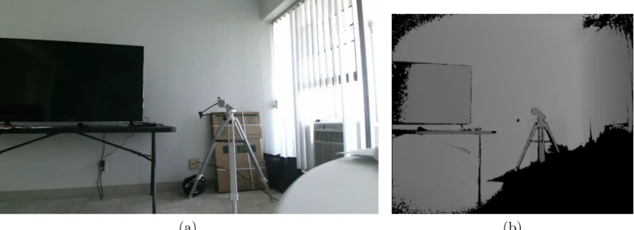
Notice that if a pixel in the RGB image is not mapped to any pixel in the depth image, then the corresponding pixel in the mapped depth image is completely black. Depth value missing is due to three reasons. The first reason is the difference in resolution. Since the RGB image has a higher resolution, some adjacent pixels in the RGB image can be mapped to one single pixel in the depth image. If they happen to be mapped to a pixel in the depth image that does not contain any depth information, black lines will appear across these pixels in the mapped depth image.

(a) (b)

Figure 3-3: Images captured by Kinect V2: (a) RGB image (1920 × 1080), (b) depth image (512 × 424). Dimensions of two images are different. Black area indicates missing depth values.

(a) (b)

Figure 3-5: Zoom-in comparison between the original depth image (a) and the smoothed depth image (b). The black pixels that indicate no depth values in (a) diminish in (b).

The second reason is the difference in field of views. The RGB camera has a field of view of 84.1 × 53.8 degrees while the depth camera only has a field of view of 70.6 × 60 degrees. Since the RGB camera has a larger field of view, some objects that are only captured by the RGB camera cannot find their corresponding depth pixels in the depth image, which causes two black strips at both ends of the mapped

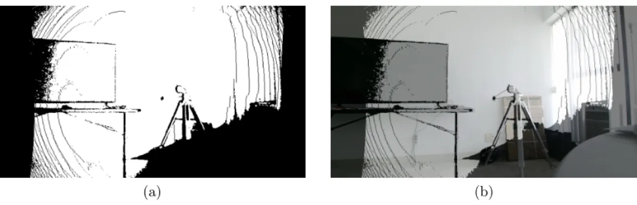
(a) (b)

Figure 3-4: Coordinate mapper maps RGB image onto depth image: (a) mapped depth image, (b) overlaid image. The black spherical lines are due to different res-olutions. The two black strips at both sides are due to differences of field of views. The black triangular region of the lower right corner is due to non-measurable depth and environment interference.

image. The third reason is the limit of Kinect’s depth measurement accuracy. If an object is outside of Kinect’s depth measurement range or depth information is missing because of the poor lighting condition, then coordinate mapper will fail to find the corresponding depth pixels. At the lower left corner of the image, the corner of round table that the Kinect sits on is closer than the shortest measurable distance of Kinect and the poor lighting condition before the tripod affects the measurement. Therefore, there is a triangular region that contains no information in the depth image and results in a black triangular region in the mapped depth image. In order to improve accuracy, we will smooth the depth image. We fill in pixels that contain no depth values with the average depth of their adjacent pixels, and the improvement after smoothing is demonstrated in Figure 3-5.

Chapter 4

Software Components

In this chapter, we outline the design and implementation of the software components of VLAMS. The data passed into the software back-end are aligned and then color enhanced for lesion segmentation. After that, area calculation is performed and the output is used to trace progress. All the codes in the project are written in Python 2.7 with image processing library OpenCV 3.2. Further details will be discussed in the following subsections.

4.1

Image Alignment and Registration

Image alignment and registration are trivial because depth images and RGB images have been pre-processed when captured. Coordinate mapper returns the mapping between pixels in the RGB image and pixels in the depth image. The index of the depth value that corresponds to the pixel with coordinate (𝑥, 𝑦) in the RGB image is given by:

4.2

Contrast Enhancement

Skin depigmentation is visually different on various types of skin. Vitiligo lesions on lighter skin are less distinguishable than those on darker skin. Thus, it is essential to incorporate a contrast enhancement tool in VLAMS to help identify lesions so that we can accurately trace the progress.

4.2.1

Gamma Correction

Gamma correction [13] is a simple nonlinear transformation. Consider an input pixel 𝐼(𝑥, 𝑦) and its corresponding output pixel 𝑂(𝑥, 𝑦), the gamma transformation follows:

𝑂(𝑥, 𝑦) = [𝛼 * 𝐼(𝑥, 𝑦) + 𝛽]1𝛾

where 𝛼 operates as an intensity amplifier, 𝛽 a range shift, and 𝛾 the gamma coeffi-cient.

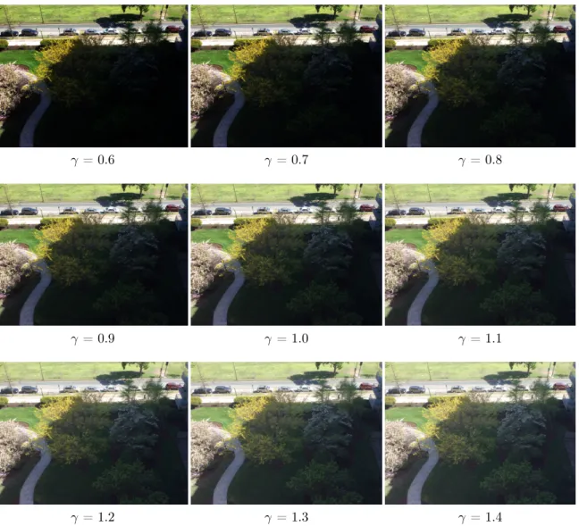
The difference in intensity between two pixels will be accentuated if 𝛾 < 1 and lessened if 𝛾 > 1. The original image is returned when 𝛾 = 1. This simple transfor-mation in intensity involves only three parameters and therefore it is computationally efficient yet powerful. In VLAMS, gamma correction is applied to all three color chan-nels independently. The effect of 𝛾 correction is demonstrated in Figure 4-1 using a landscape shot taken in the afternoon when the shadow and highlights conceal a lot of details.

4.2.2

Histogram Equalization

A histogram is a graphical representation of the pixel intensity in the image. The left side of the graph represents the information of darker area in the image and the right side represents the brighter area. The height of each bar indicates the frequency of the pixels in the specific intensity range, typically from 0 to 255.

𝛾 = 0.6 𝛾 = 0.7 𝛾 = 0.8

𝛾 = 0.9 𝛾 = 1.0 𝛾 = 1.1

𝛾 = 1.2 𝛾 = 1.3 𝛾 = 1.4

Figure 4-1: Gamma correction with no amplification and shift (𝛼 = 1.0, 𝛽 = 1.0). Notice that 𝛾 = 1.0 represents the original image.

Consider a grayscale input image 𝑋 with gray levels ranging from 0 to 𝐿−1. From a probabilistic model point of view, each bar in histogram represents the probability density of pixels with gray level 𝑖. Define the cumulative distribution function 𝐹𝑋(𝑖)

of pixels with intensity level 𝑖:

𝐹𝑋(𝑖) = 𝑖 ∑︁ 𝑗=0 𝑛𝑗 𝑛

where 𝑛𝑗 is the number of pixels with gray level 𝑗 and 𝑛 the total number of pixels

Histogram equalization [14] converts the input image to the output image 𝑌 such that 𝐹𝑌(𝑖) is linear. Given the linearity of cumulative distribution function 𝐹𝑌(𝑖), we

can see that the mass density function 𝑓𝑌(𝑖) = (𝐹𝑌(𝑖))′ is constant. This spreads out

the most frequent intensity values in the image and therefore increases global contrast of the image. The effect of the histogram equalization is demonstrated in Figure 4-2.

Original image Image after histogram equalization

Figure 4-2: Image before and after histogram equalization with corresponding his-togram. In the original image, histogram skews to the right, which indicates a poten-tial of over exposure. By equalizing histogram, a more evenly distributed histogram is achieved. More details in the shadow and the highlight are now visible in the image.

4.2.3

CLAHE

Histogram equalization in the previous section considers the global contrast of the image. However, in many cases, it is sub-optimal. An improved technique known as adaptive histogram equalization [15] is used to provide better contrast processing. Adaptive histogram equalization divides images into tiles with a much smaller size than the dimension of the image. Each tile is first histogram equalized and combined. Then bilinear interpolation is applied to soften tile borders.

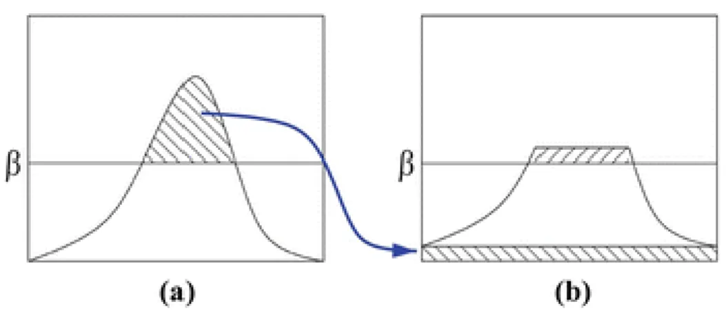
Adaptive histogram equalization produces excellent results in enhancing the signal component of an image, but it also amplifies the noise in the image. To address this problem, contrast limitation is introduced. In the contrast limited adaptive histogram equalization, or CLAHE, a contrast limit threshold 𝛽 is specified. If any histogram bin is beyond 𝛽, the corresponding pixels will be clipped and distributed evenly into other bins before histogram equalization, as shown in Figure 4-3. The comparison between histogram equalization and CLAHE is shown in Figure 4-4.

Figure 4-3: Contrast limitation is applied to avoid amplifying noise. Values that are beyond threshold 𝛽 in (a) are clipped and distributed in (b) [16].

Original Image Histogram Equalization CLAHE

Figure 4-4: Images with their corresponding histograms underneath. The original image focuses on artistic expression while details are ignored. On the right, the chair is not recognizable in the original image. After histogram equalization, the chair is more visible but the details on the canvas are lost. By applying CLAHE, chair becomes more visible and details on the canvas are preserved. The difference can also be inferred from the changes in the histogram. CLAHE shapes the histogram more evenly and smoothly than normal equalization.

4.2.4

Lab Color Space

Lab color space is designed to approximate human vision. It describes perceivable colors using three parameters: L for lightness, a for green-red color opponents and b for blue-yellow color opponents, as shown in Figure 4-5. By converting the original image from RGB color space to Lab color space, VLAMS can adjust the lightness layer to reveal hidden details that are not apparent, without losing the color features. After the adjustment, Lab image will be converted back into RGB image for further processing. Lab color space has been used in previous research [17] [18] for image segmentation. For this reason, we decide to provide user the option to perform color

adjustment in Lab color space to increase segmentation accuracy.

RGB L channel

a channel b channel

Figure 4-5: RGB image converted into Lab color space. L channel stores the lightness information while a and b channels store color information.

4.2.5

Integrated Tool

In the previous sections, all the methods incorporated in the contrast enhancer along with their working mechanisms have been introduced. VLAMS provides an integrated tool that allows users to efficiently enhance contrast and reveal unapparent details. It provides a variety of options for users to select, including whether to operate in Lab color space, perform gamma correction and different modes of histogram equalization. The user interface along with the sample processing image is shown in Figure 4-5.

Figure 4-6: An example of processing a vitiligo lesion image using contrast enhancer. The original image is on the left and enhanced image on the right. After applying CLAHE in Lab color space and with some gamma correction, more hidden vitiligo lesions become apparent. Notice on the upper left corner, lesions are barely noticeable in the original image. The ranges for 𝛼, 𝛽 and 𝛾 are 0−3, 0−100 and 0−3 respectively.

4.3

Lesion Segmentation

VLAMS adopts two different segmentation algorithms, thereby providing flexibility and interactivity.

4.3.1

Grabcut

Grabcut [19] is an image segmentation method based on graph cuts. For an object that can be specified within a box, grabcut can perform lesion segmentation reliably. The algorithm can be described as follows:

1. User specifies a rectangle box that bounds the object. Everything outside is taken as sure background.

2. Algorithm initializes labelling of the foreground and background pixels. User can also correct background and foreground labelling manually.

3. A Gaussian Mixture Model (GMM) is used to model the foreground and back-ground.

4. A graph is built from this pixel distribution. In the graph, the pixels are nodes and weights of edges connecting two nodes depend on pixel similarity.

5. A min-cut algorithm is performed to segment the graph into foreground and background.

6. Step 3-5 are repeated until convergence.

An example piece of A3 paper segmented using Grabcut algorithm is presented in Figure 4-7. First, a rectangle box is drawn to bound the A3 paper, then black markers are drawn to indicate sure background and white markers are drawn to show sure foreground. After a few iterations, the whole A3 paper is clearly segmented. Notice that the reflection on the marble is well separated from the real A3 paper.

4.3.2

Watershed

Grabcut algorithm does not perform as expected on objects that are not bounded or on multiple objects given its very nature. This drives us to find an alternative -watershed algorithm [20]. The name of -watershed algorithm refers metaphorically to a geological watershed, which separates adjacent drainage, like two components in a graph. Similar to grabcut algorithm, watershed allows users to select background and foreground so that the image can be more accurately segmented. But the drawback of watershed algorithm is its efficiency. Since the algorithm is run on the whole image instead of in a specified region, it requires more user intervention.

(a) (b)

(c) (d)

Figure 4-7: A3 paper segmentation using grabcut algorithm. (a) The original RGB image. (b) A rectangle box is drawn to bound the object for segmentation. (c) Markers of different colors used to indicate background and foreground. (d) Final output.

An image with multiple lesions is used to demonstrate the difference in perfor-mance between grabcut and watershed. First, the image is contrast enhanced in order to expose all the details for segmentation. Grabcut algorithm tends to connect all four different lesions into one whole lesion and therefore results in a smoother bound-ary for each lesion. On the other hand, watershed gives finer boundaries while it requires a lot of manual labelling for initialization. We compare the performance of both segmentation methods with a manually segmented lesion image as the ground truth. The accuracy of each segmented area is defined as the ratio of overlapped area in pixels to the ground truth area in pixels. We also compare segmentation

based on the contrast-enhanced image and the original image as cross-validation to show that contrast enhancement does improve segmentation accuracy. The segmen-tation comparison is shown in Figure 4-8. The comparison between accuracy of two segmentation methods is listed in Table 4.1.

(a) (b)

(c) (d)

(g)

Figure 4-8: Comparison between Grabcut and Watershed on multiple lesions. (a) The original RGB image. (b) Image after contrast enhancement. (c) Grabcut segmenta-tion based on the contrast-enhanced image. (d) Watershed segmentasegmenta-tion based on the contrast-enhanced image. (e) Grabcut segmentation based on the original image. (f) Watershed segmentation based on the original image. (g) The ground truth.

Watershed Algorithm Grabcut Algorithm Accuracy (original image) 72.08 % 73.61 % Accuracy (contrast-enhanced image) 92.06 % 85.77 %

Table 4.1: Comparison between two segmentation algorithms based on the contrast-enhanced image and the original image.

4.4

Area Calculation

After lesion segmentation, the final step remaining is to calculate the lesion area. A naive method for calculating area is to count the number of pixels a lesion takes up. This naive method fails for two reasons. First, on a curved surface, only the projected surface area is captured. Second, the size of a lesion in the image changes with distance. The longer the distance the smaller size it appears in the image. It therefore requires the image to be taken at a very specific distance in order to track the progress, which is technically difficult. Using the depth information VLAMS col-lects along with the RGB image, VLAMS can make use of this depth information to calculate the real area in squared millimeter instead of relative area in pixels.

Figure 4-9: If area is directly calculated from the RGB image without depth infor-mation, the area of projection 𝑇 instead of the actual surface area 𝑆 (dark grey) is obtained [21].

Let’s consider the case in which the lesion 𝑆 in the image is to be measured, as shown in Figure 4-9. Assume the sensor plane lies in the X-Y plane, then any point 𝑃 = (𝑥, 𝑦, 𝑧) = (𝑥, 𝑦, 𝐷(𝑥, 𝑦)) on lesion indicates that the point lies on the RGB image with coordinate (𝑥, 𝑦) with a depth value 𝐷(𝑥, 𝑦). The depth value can be obtained by calculating the depth index as introduced in section 4.1. Mathematically, the surface integral of 𝑆 is given by:

𝐴 = ∫︁ ∫︁ 𝑇 ⃦ ⃦ ⃦ ⃦ (︂ 1, 0,𝜕𝐷 𝜕𝑥 )︂ × (︂ 0, 1,𝜕𝐷 𝜕𝑦 )︂⃦ ⃦ ⃦ ⃦ d𝑥 d𝑦 = ∫︁ ∫︁ 𝑇 √︃ (︂ 𝜕𝐷 𝜕𝑥 )︂2 +(︂ 𝜕𝐷 𝜕𝑦 )︂2 + 1 d𝑥 d𝑦

If the gradient for 𝑧 direction is missing (𝜕𝐷_𝜕𝑥 = 𝜕𝐷_𝜕𝑦 = 0), then it is the same as performing a surface integral in two dimensional space using only RGB image, which

gives the projected surface area 𝑇 instead: 𝐴 = ∫︁ ∫︁ 𝑇 ⃦ ⃦ ⃦ ⃦ (︂ 1, 0,𝜕𝐷 𝜕𝑥 )︂ × (︂ 0, 1,𝜕𝐷 𝜕𝑦 )︂⃦ ⃦ ⃦ ⃦ d𝑥 d𝑦 = ∫︁ ∫︁ 𝑇 1 d𝑥 d𝑦 = 𝑇

The surface integral takes a continuous depth function, but data from the hard-ware is discrete. For this reason, VLAMS calculates surface area using discrete ap-proximation. Consider that the hardware has a field of view 𝐹𝑥× 𝐹𝑦 degrees with

a resolution of 𝑅𝑥× 𝑅𝑦 pixels. Assume that the camera is ideal without distortion,

then each pixel corresponds to a field of view of 𝜃𝑥× 𝜃𝑦 degrees where 𝜃𝑥 = 𝐹𝑥/𝑅𝑥 and

𝜃𝑦 = 𝐹𝑦/𝑅𝑦. Consider that a projected surface ∆𝑆 with width ∆𝑥 and height ∆𝑦 at

distance 𝐷 is captured in one single pixel. Assume that both 𝜃𝑥 and 𝜃𝑦 are small, then

by trigonometry, ∆𝑥 = 𝐷𝜃𝑥 and ∆𝑦 = 𝐷𝜃𝑦. Thus, we have ∆𝑆 = ∆𝑥∆𝑦 = 𝐷2𝜃𝑥𝜃𝑦,

as shown in Figure 4-10.

Figure 4-10: One single pixel captures a projected area ∆𝑆 at distance 𝐷.

Since the surface is not necessarily flat, we also need to incorporate the gradient of the depth in order to give better approximation. The gradient of depth at pixel (𝑖, 𝑗) can be approximated using central difference theorem. Consider three horizontally

aligned pixels (𝑖 − 1, 𝑗), (𝑖, 𝑗), and (𝑖 + 1, 𝑗) that correspond to physical locations 𝑥 − 𝑡, 𝑥 and 𝑥 + 𝑡. These locations have distances 𝐿(𝑥 − 𝑡), 𝐿(𝑥), and 𝐿(𝑥 + 𝑡) respectively, where 𝐿(𝑥) = 𝐷(𝑖, 𝑗), as shown in Figure 4-11. Given that a single pixel has a horizontal field angle of 𝜃𝑥, we can see that 𝑡 = 𝐷𝜃𝑥. Then, at location 𝑥 or

pixel (𝑖, 𝑗), the horizontal gradient approximation is given by:

𝜕𝐿(𝑥) 𝜕𝑥 ≈ 𝐿(𝑥 + 𝑡) − 𝐿(𝑥 − 𝑡) 2𝑡 = 𝐷(𝑖 + 1, 𝑗) − 𝐷(𝑖 − 1, 𝑗) 2𝐷(𝑖, 𝑗)𝜃𝑥 ≡ 𝐷𝑥(𝑖, 𝑗)

using the same argument, the vertical gradient approximation is given by:

𝜕𝐿(𝑦) 𝜕𝑦 ≈ 𝐿(𝑦 + 𝑡) − 𝐿(𝑦 − 𝑡) 2𝑡 = 𝐷(𝑖, 𝑗 + 1) − 𝐷(𝑖, 𝑗 − 1) 2𝐷(𝑖, 𝑗)𝜃𝑦 ≡ 𝐷𝑦(𝑖, 𝑗)

Figure 4-11: Example of using central difference to approximate gradient. Three pixels (𝑖 − 1, 𝑗), (𝑖, 𝑗), and (𝑖 + 1, 𝑗) correspond to three physical location 𝑥 − 𝑡, 𝑥 and 𝑥 + 𝑡. The gradient (green) at point (𝑥, 𝐿(𝑥)) is approximated by the slope (red) of the line connecting point (𝑥 − 𝑡, 𝐿(𝑥 − 𝑡)) and point (𝑥 + 𝑡, 𝐿(𝑥 + 𝑡)).

Therefore the surface area is the sum of the area of each pixel in the lesion and can be written as:

𝐴 ≃ ∑︁

𝑝∈𝐿𝑒𝑠𝑖𝑜𝑛

𝐷(𝑝)2 √︁

Once the lesion area is obtained, it can be stored in a clinical database for progress tracking.

Chapter 5

Performance

In this chapter, we test the performance of VLAMS on both test data and medical data.

5.1

Test Data

5.1.1

Area Calculation

In order to test the accuracy of area calculation in VLAMS, we measure a box with known surface area at different distances. This box has a surface area of 524.80 𝑚𝑚2, and this comparison gives us intuitive understanding of the performance of VLAMS. The experiment set-up is shown in Figure 5-1.

The test results are shown in Table 5.1 and the relative error is plotted in Figure 5-2. From the results, we see that Kinect V1 has its optimal measurement at around 0.6 𝑚 while Kinect V2 has its optimal measurement at around 0.9 𝑚. After they reach the optimal points, both Kinect V1 and Kinect V2 have worse measurements as the distance increases. The reason that Kinect V1 obtains worse measurement as it gets further is due to the very nature of the depth measurement. Kinect V1 uses stereo effect for depth measurement and it gets less sensitive to distance for an object that is further. As for Kinect V2, measurement gets less accurate as object

(a)

(b) (c)

Figure 5-1: Measurement of a box with known surface area at 914 mm (approximately 3 ft). Image taken by Kinect V2. The ruler on the floor helps locate the distance. (a) The RGB image. (b) Overlaid with mapped depth image. (c) Segmentation result.

gets further from 0.9 𝑚 and is inaccurate when it is less than or equal to 0.6 𝑚. This is due to the very nature of time-of-flight measurement - the depth measured is the speed of light times the time needed by the photon to travel from emitter to target. If the distance is very short, the photon travel time will also be very short. Thus, the systematic error in time measurement becomes relatively more significant and results in an inaccurate measurement. If the distance is too far, then the light path gets more interfered by the environment, which compromises the accuracy.

Distance (mm) 609 762 914 1067 1219 1371 Area from Kinect V1 (𝑚𝑚2_{) 492.11 487.16 491.70 464.86 463.56 461.53}

Area from Kinect V2 (𝑚𝑚2_{) 437.64 504.94 507.88 490.30 494.41 479}

Figure 5-2: Measurement error at different distance.

5.1.2

Lesion Segmentation

In this section, we evaluate the robustness of lesion segmentation. We use the same data set from [9] that consists of clinical images captured over two years. For com-parison purposes, we select a series of three images of the same vitiligo lesion over a period of time.

Results are shown in Figure 5-3 to Figure 5-5. For each image, we add a reference image that is manually segmented for accuracy comparison. The accuracy is defined as the ratio of the overlapped area between segmented area and the ground truth area in pixels to the the ground truth area in pixels, and they are listed in Table 5.2 to Table 5.4. These results show that the robustness of VLAMS on lesion segmentation meets our expectation, and VLAMS can consistently output desired lesion segmentation for further progress tracking.

(a) (b)

(c) (d)

Figure 5-3: Lesion segmentation comparison. (a) The original image. (b) The ground truth. (c) Result from VLAMS. (c) Results from [9].

Segmentation from VLAMS Segmentation from [9] Accuracy (%) 96.78 91.57

(a) (b)

(c) (d)

Figure 5-4: Lesion segmentation comparison. (a) The original image. (b) The ground truth. (c) Result from VLAMS. (c) Results from [9].

Segmentation from VLAMS Segmentation from [9]

Accuracy (%) 89.5 89.4

(a) (b)

(c) (d)

Figure 5-5: Lesion segmentation comparison. (a) The original image. (b) The ground truth. (c) Result from VLAMS. (c) Results from [9].

Segmentation from VLAMS Segmentation from [9]

Accuracy (%) 85.9 83.3

5.2

Medical Data

In this section, we evaluate the accuracy of VLAMS and validate its accuracy on clin-ical data. All data are collected on-site at Brigham and Women’s Hospital/Faulkner with Dr. Victor Huang. For comparison purposes, planimetry measurements for each lesion are also recorded at the same time. Notice that planimetry measurement result are not perfectly accurate and the sources of error may come from manual segmenta-tion, inaccuracy of planimetry machine, and thickness of the markers etc. However, since planimetry measurements are the most adopted method used in clinical mea-surement, we use the results from planimetry measurement results as comparison benchmarks.

We successfully collect data from three patients. For privacy reasons, we have pro-cessed and cropped the images to hide the identities of the patients. In the following patient reports, the post-its contain trios of measurements for each measurable lesion – surface area, largest width, and largest height. In terms of the tracings themselves, the dotted lines are areas where the clinical borders were fuzzy.

1. Patient 1

Patient Description:

Male. Patient has dark skin type. Lesion is at anterior neck. Repigmentation within the lesion is visually apparent but is not included in planimetry mea-surement due to the resolution limit of the planimetry machine. Slight contrast enhancement is made to help segmentation. Expected to have a close VLAMS measurement compared to planimetry measurement. Results show a 7% differ-ence.

Result :

(a)

(b) (c)

Figure 5-6: Lesion segmentation: (a) original RGB image, (b) segmentation on en-hanced image, (c) segmentation on original image.

(a) (c)

Figure 5-7: Lesion comparison: (a) lesion in the image, (b) tracing on cellophane.

Planimetry Measurement VLAMS Measurement Difference (%) 1.80 cm2 _{1.67 cm}2 ₇

Table 5.5: Area measurement comparison.

2. Patient 2

Patient Description:

Female. Patient has very light skin type. Lesion is at right cheek. Discontinu-ities are slightly observable. Due to the curvature of patient’s cheek, tracings on cellophane do not look similar to the lesion in the image. No contrast en-hancement is made. Expected to have a close VLAMS measurement compared to planimetry measurement. Results show a 4% difference.

(a) (b)

Figure 5-8: Lesion segmentation: (a) original RGB image, (b)segmentation on original image.

(a) (b)

Figure 5-9: Lesion comparison: (a) lesion in the image, (b) tracing on cellophane. The tracings are drawn on a curved surface, and when flattened on cellophane, they appear differently from the image.

Planimetry Measurement VLAMS Measurement Difference (%) 8.8 cm2(total) 8.43 cm2 4

Table 5.6: Area measurement comparison.

3. Patient 3

Male. Patient has light skin type. Lesions are symmetrical on both nasolabial folds. Contrast enhancement is made to help segmentation, showing more vi-tiligo lesions on the forehead. A huge part of the lesion is only visible under ultra-violet light and is captured under normal light condition. Tracings are drawn using an ultra-violet lamp. Expected to have a different VLAMS mea-surement compared to planimetry meamea-surement but lesions on both sides have similar size.

Result :

(a)

(b) (c)

Figure 5-10: Lesion segmentation: (a) original RGB image, (b) segmentation on enhanced image, (c) segmentation on original image.

(a) (b)

Figure 5-11: Lesion comparison: (a) lesion in the image, (b) tracing on cellophane.

Planimetry Measurement VLAMS Measurement Difference (%) 9.70 (L) cm2 5.25 (L) cm2 46 (L) 8.90 (R) cm2 _{4.72 (R) cm}2 _{47 (R)}

Chapter 6

Conclusion

In this chapter, we summarize VLAMS’s contribution to the medical imaging field and discuss future improvements to VLAMS.

6.1

Contribution

This thesis presents a new solution to surface area measurement of vitiligo lesions by incorporating a depth camera and image processing algorithms. We show that VLAMS can perform lesion segmentation robustly and measure lesion area accurately over any skin surface. Compared to the currently existing approaches mentioned in section 1.2, VLAMS has several advantages.

First of all, VLAMS is easy to use. VLAMS does not require any precise cali-bration or professional training. Secondly, VLAMS is contact-free. This eliminates the possibility of contamination and discomfort caused by manual tracing. Thirdly, VLAMS is environment-friendly. Unlike the Visitrak system, each grid sheet is dis-posed after use, VLAMS does not produce any waste. Lastly, VLAMS can measure area of any surface and output absolute value of area for further analysis.

However, the data set we had for validation is small. Larger data sets are essential to fully test out VLAMS. We hope the development of VLAMS will inspire medical

devices in the future.

6.2

Challenges

Data collection for this project is challenging. Frequently, patients who have made appointments do not show up, thereby limiting the size of our data set. Given the time span of this project, we did not get a chance to trace the progress of each patient over a longer period.

6.3

Future Work

There are a number of research directions that can be pursued to improve the robust-ness of VLAMS.

6.3.1

Better Camera with Higher Resolution

The resolution of the depth image is crucial to calculating the surface area. Con-sider the very extreme case where the resolution of the depth camera is 1 × 1. By coordinate mapping, all RGB pixels will have the same corresponding depth value, which is not desirable. On the other hand, if we have cameras with higher resolution, we would be able to capture more depth information and thus the curvature can be better modeled by VLAMS.

The difference in data capture is shown in Figure 6-1. Consider that a curved surface 𝑆 is the target surface and its area needs to be calculated. Using a camera with low resolution, only four points (marked in orange) are sampled. Unfortunately, these four points lie on the same plane. Since the system only sees these four points, the gradient of 𝑆 is calculated to be zero and a projected surface area (dashed line) is obtained in this way. However, if a camera with higher resolution is used, more points on surface 𝑆 are sampled. Now, the curvature of 𝑆 is better captured and by

using central difference, we can obtain a more accurate measurement of the gradient and therefore a better estimation of the surface area.

(a)

(b)

Figure 6-1: Cameras with different resolution: (a) camera with a low resolution can only sample 4 points on a curved surface, (b) camera with a high resolution can sample 9 points.

6.3.2

Depth Frame Reconstruction

In [22], Natalia, Damien, and Alain propose a method for restoring precise depth information from a single depth image. This methods performs well even under the condition of low resolution and presence of noise. Currently in VLAMS, missing depth values are filled by averaging the adjacent depth values. But if a huge block of the

depth image is missing depth information, the accuracy of area measurement will be compromised. Thus, by incorporating this aforementioned optimization method, we can enhance the robustness of VLAMS.

6.3.3

Additional Lighting Option

In section 5.2, we see that if a lesion is not visible under normal lighting, additional lighting such as ultra-violet will be needed. We recommend that clinics provide dif-ferent lighting during image capture with VLAMS. Only when the whole lesion is exposed, can an accurate measurement of the lesion size be made.

6.3.4

Visualization of Progress

Currently, VLAMS does not have the capability to capture the animation of the same lesion over time. One potential solution to this is to incorporate scale-invariant feature transform (SIFT) algorithm [23] into VLAMS. SIFT allows us to detect corresponding features across a series of images of the same lesion taken at different times. We can then align and stack the images based on these extracted features to create an animation, which helps doctors visualize how the lesion progresses.

Bibliography

[1] Rithe, Rahul Rahulkumar Jagdish. Energy-efficient system design for mobile processing platforms. Diss. Massachusetts Institute of Technology, 2014. [2] Zhang, Yiwei, et al. "A fast 3D reconstruction system with a low-cost camera

accessory." Scientific reports 5 (2015).

[3] http://www.smith-nephew.com/new-zealand/healthcare/products/product-types/visitrak/

[4] http://wound.smith-nephew.com/CA_EN/node.asp?NodeId=3053 [5] National Institutes of Health. Image J software. Available from: URL:

http://imagej.nih.gov.

[6] Schneider, Caroline A., Wayne S. Rasband, and Kevin W. Eliceiri. "NIH Image to ImageJ: 25 years of image analysis." Nature methods 9.7 (2012): 671.

[7] Shetty, Rahul, et al. "A novel and accurate technique of photographic wound measurement." Indian Journal of Plastic Surgery 45.2 (2012): 425.

[8] Chang, Angela Christine, Bronwyn Dearman, and John Edward Greenwood. "A comparison of wound area measurement techniques: visitrak versus photography." Eplasty 11.18 (2011): 158-66.

[9] Sheth, Vaneeta M., et al. "A pilot study to determine vitiligo target size using a computer-based image analysis program." Journal of the American Academy of Dermatology 73.2 (2015): 342-345.

[10] http://www.xbox.com/en-US/xbox-one/accessories/kinect

[11] Khoo, Rachel, and Shirley Jansen. "The Evolving Field of Wound

Measurement Techniques: A Literature Review." Wounds: a compendium of clinical research and practice 28.6 (2016): 175.

[12] Zhang, Zhengyou. "A flexible new technique for camera calibration." IEEE Transactions on pattern analysis and machine intelligence 22.11 (2000): 1330-1334.

[13] Lee, Dong-U., Ray CC Cheung, and John D. Villasenor. "A flexible

architecture for precise gamma correction." IEEE Transactions on Very Large Scale Integration (VLSI) Systems 15.4 (2007): 474-478.

[14] Rafael C. Gonzalez and Richard E. Woods. 2006. Digital Image Processing (3rd Edition). Prentice-Hall, Inc., Upper Saddle River, NJ, USA.

[15] Pizer, Stephen M., et al. "Adaptive histogram equalization and its variations." Computer vision, graphics, and image processing 39.3 (1987): 355-368.

[16] Al-Ameen, Zohair, et al. "An innovative technique for contrast enhancement of computed tomography images using normalized gamma-corrected

contrast-limited adaptive histogram equalization." EURASIP Journal on Advances in Signal Processing 2015.1 (2015): 32.

[17] Achanta, Radhakrishna, et al. "SLIC superpixels compared to state-of-the-art superpixel methods." IEEE transactions on pattern analysis and machine intelligence 34.11 (2012): 2274-2282.

[18] Bansal, Seema, and Deepak Aggarwal. "Color image segmentation using CIELab color space using ant colony optimization." International Journal of Computer Applications 29.9 (2011): 28-34.

[19] Carsten Rother, Vladimir Kolmogorov, and Andrew Blake. 2004. "GrabCut": interactive foreground extraction using iterated graph cuts. In ACM

SIGGRAPH 2004 Papers (SIGGRAPH ’04), Joe Marks (Ed.). ACM, New York, NY, USA, 309-314. DOI=http://dx.doi.org/10.1145/1186562.1015720 [20] Roerdink, Jos BTM, and Arnold Meijster. "The watershed transform:

Definitions, algorithms and parallelization strategies." Fundamenta informaticae 41.1, 2 (2000): 187-228.

[21] https://en.wikipedia.org/wiki/File:Surface_integral1.svg

[22] Neverova, Natalia, Damien Muselet, and Alain Tremeau. "21/2 d scene

reconstruction of indoor scenes from single rgb-d images." Computational Color Imaging. Springer Berlin Heidelberg, 2013. 281-295.

[23] Lowe, David G. "Object recognition from local scale-invariant features." Computer vision, 1999. The proceedings of the seventh IEEE international conference on. Vol. 2. Ieee, 1999.