Estimates of the modeling error generated by homogenization of an elliptic boundary value problem

Sergey Repin*, Tatiana Samrowski, and Stefan Sauter

Estimates of the modeling error generated by

homogenization of an elliptic boundary value

problem

Abstract: In this paper, we derive a posteriori bounds of the difference between the exact solution of an elliptic boundary value problem with periodic coefficients and an abridged model, which follows from the homog-enization theory. The difference is measured in terms of the energy norm of the basic problem and also in the combined primal–dual norm. Using the technique of functional type a posteriori error estimates, we ob-tain two-sided bounds of the modeling error, which depends only on known data and the solution of the homogenized problem. It is proved that the majorant with properly chosen arguments possesses the same convergence rate, which was established for the true error. Numerical tests confirm the efficiency of the esti-mates.

Keywords: periodic structures, homogenization, elliptic boundary value problems, a posteriori error esti-mates, modeling error

MSC 2010: 35J15, 35B27, 65N15

DOI: 10.1515/jnma-2014-1002

Received January 26, 2014; revised November 21, 2014; accepted January 28, 2015

1 Introduction

Boundary value problems with periodic structures arise in various applications. Homogenization theory is the major tool used to quantitatively analyze media with periodic structures. Within the framework of the theory (see, e.g., [9, 14]), the behavior of a heterogeneous media is described with the help of a certain homogenized problem, which is typically a boundary value problem with smooth coefficients, and the solution of a specially constructed problem with periodic boundary conditions. It has been proved that the functions reconstructed by this procedure converge to the exact solution as the cell size ε tends to zero. Moreover, known a priori error estimates qualify the convergence rate in terms of ε. The goal of this paper is to derive two-sided estimates of the modeling error generated by homogenization. In other words, we wish to estimate the difference between the exact solution of the original problem and its approximation obtained by the corresponding homogenized model.

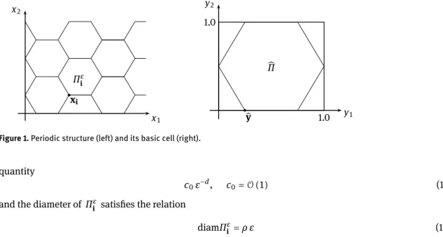
Let Ω ⊆ ℝd be a bounded domain with Lipschitz boundary ∂Ω, such that Ω = ⋃iΠiε, where

Π_iε= xi+ ε ̂Π = {x ∈ ℝd󵄨󵄨󵄨_󵄨󵄨󵄨 x − xi ε ∈ ̂Π}

is the basic ‘cell’ (repeating element of the periodic structure, see Fig. 1), which is a simply connected domain with Lipschitz boundary, xi is the reference point of Π_iε, and ε is a small parameter (geometrical size of a cell). Here and later on, x denotes the global (Cartesian) coordinate system in ℝd_{and i = (i}

1, i2, . . . , id)

denotes the counting multi-indices for the cells. The notations ⋃iand ∑iare shorthands for the union and summation over all cells. It is assumed that the overall amount of Π_iε in Ω is bounded from above by the

*Corresponding Author: Sergey Repin: V. A. Steklov Institute of Mathematics, Fontanka 27, 191011 St. Petersburg, Russia, and

University of Jyväskylä, Finland. Email: repin@pdmi.ras.ru

Tatiana Samrowski: Institute for Applied Mathematics and Physics, Zurich University of Applied Sciences, Technikumstrasse 6,

CH-8400 Winterthur, Switzerland

x₁ x₂ ∙_x i Π_iε y₁ y₂ 1.0 1.0 ̂y ∙ ̂Π

Figure 1. Periodic structure (left) and its basic cell (right).

quantity

c0ε−d, c0=O (1) (1.1)

and the diameter of Π_iε satisfies the relation

diamΠε_i = ρ ε (1.2)

where ρ is a parameter depending on the geometry of the cell. Usually, ρ is easy to find (e.g., for a cubic cell

ρ = √d ).

In the basic cell (see Fig. 1), we use local Cartesian coordinates y ∈ ℝd_{. For any Π}ε

i , local and global coordinates are joined by the relation

y = x − xi

ε ∈ ̂Π ∀ x ∈ Π ε

i, ∀ i.

On ̂Π, we define a matrix function ̂A ∈ L∞_{(̂Π, ℝ}d×d

sym), where ℝsymd×ddenotes the set of symmetric d ×

d-matrices. We assume that

c1|ξ|2 ⩽ ̂A(y)ξ ⋅ ξ ⩽ c2|ξ|2 ∀ ξ ∈ ℝd, ∀ y ∈ ̂Π (1.3)

where 0 < c1⩽ c2< ∞ and introduce the ‘global’ matrix

Aε(x) := ̂A (x − xi

ε ) ∀ x ∈ Π ε

i, ∀ i (1.4)

which defines the periodic structure on Ω. In view of (1.3), Aε(and its inverse counterpart A−1ε ) satisfy similar

two-sided estimates for any ε.

Consider the second-order elliptic equation

− div (Aε∇uε) = f in Ω, f ∈ L2(Ω) (1.5)

with homogeneous Dirichlet boundary conditions. The corresponding generalized solution uε ∈ H1₀(Ω) is

defined by the relation

∫

Ω

Aε∇uε⋅ ∇w = ∫ Ω

fw ∀ w ∈ H₀1(Ω) . (1.6)

For any ε > 0, the solution uε exists and is unique.

For a function ζ ∈ L1(ω), where ω is a measurable subset of Ω, we define the mean value by ⟨ζ⟩ω:=

1 |ω|∫ω

ζ. (1.7)

If no confusion may arise, we omit in integrals the symbol of the corresponding Lebesque measure (e.g., dx). However, we write the measure explicitly if it is necessary to distinguish between integration over the global and local coordinates (as in Lemma 2.1).

If we write ∫_ω⟨ζ⟩ω, then the average is considered as a constant function on ω (for vector-valued

func-tions, we apply this definition componentwise). The error caused by the averaging (1.7) is denoted by

δωζ := ‖ζ − ⟨ζ⟩ω‖ω

where ‖ ⋅ ‖ω denotes the standard L2−norm on ω.

For a vector µ = (µi)d_i=1∈ (ℝ>0)dand s ∈ ℝ, µsdenotes the componentwise application of the power s,

i.e., µs = (µs_i)d_i=1. For vector-valued functions ζ = (ζk)d_k=1 ∈ L1(ω, ℝd) and φ = (φk)d_k=1∈ L1(Ω, ℝd) , we

define the local and piecewise constant averages by means of the relations

δωζ := (‖ζk− ⟨ζk⟩ω‖ω) d k=1, δ pw Ω φ := εd/2( ∑ i ‖φk− ⟨φk⟩Πε i‖Π ε i) d k=1 and (δωζ )2:= (‖ζk− ⟨ζk⟩ω‖2ω) d k=1, (δ pw Ω φ) 2 := εd ((∑ i ‖φk− ⟨φk⟩Πε i‖Πεi) 2 ) d k=1 .

Within the framework of homogenization theory, an approximation of uε is constructed by the following

procedure (see, e.g., [7, 9, 14]). First, we define (for k = 1, 2, ..., d) the solutions Nk of ‘cell problems’

div( ̂A ∇ Nk) = (div ̂A) k in ̂Π Nk is periodic in ̂Π ∫ ̂ Π Nk= 0. (1.8)

With the help of them, the homogenized matrix

A0= ⟨̂A ( I − ∇N) ⟩_̂

Π (1.9)

is defined. The function u0∈ H1₀(Ω) such that

∫

Ω

A0∇u0⋅ ∇w = ∫ Ω

f w ∀ w ∈ H₀1(Ω) (1.10)

provides a “coarse” approximation of uε. It is known that (see, e.g., [7]),

uε→ u0 in L2(Ω), uε⇀ u0 in H10(Ω) for ε → 0.

However, it is necessary to construct a sequence of more accurate approximations, which converges in a stronger sense. For this purpose, the homogenization theory suggests to use advanced approximations

w1_ε(x) := u0(x) − εψε(x) Nk( x − xi ε ) ∂ u0(x) ∂xk ∀ x ∈ Πε_i, ∀ i (1.11) where ψε_{:= min{1, dist(x, ∂Ω)/ε} is a cutoff function.}

To prove optimal a priori convergence rates for the modeling error

emod_ε := uε− w1ε (1.12)

we need some extra assumptions (see [14], p.28), namely,

u0 ∈ W2, ∞(Ω) (1.13)

and

∂ Nk ∂yj ∈ L

∞_{(̂Π). (1.14)}

Then, it can be proved (see, e.g., [7], Remark 5.13; [10]; [14], p. 28) that the modeling error satisfies the asymp-totic estimates:

and ‖Aε∇ uε− v0− ε v1‖ ⩽ ̂c √ε (1.16) where v0:= (I − curlỹN) µ µ := ⟨A−1 0 (I − curlỹN)⟩−1̂Π ∇u0 v1:= −curlx(̃N µ) (1.17)

the d × d matrix ̃N with columns ̃Nk is the solution of the auxiliary problem

curl A−1

0 ( curl ̃Nk(y)) = curl ( A−10 )_k in ̂Π

div ̃Nk= 0 ̃ Nk is periodic in ̂Π ∫ ̂ Π ̃ Nk= 0 (1.18)

and the columns of the matrix curlỹN are given by curlỹNk, k = 1, 2, . . . , d.

Numerical methods for homogenized problems are actively studied. Such questions as adaptivity and error indication are among the most important questions arising in quantitative analysis of periodical struc-tures. Here, we first of all mention residual type error indicators that develop the ideas suggested in [2, 3] for finite element approximations. Since our approach is based on a different technique, we will sketch here only briefly some relevant literature on residual based estimation and refer for a detailed review, e.g., to [13]. A posteriori error estimates for the heterogeneous multiscale discretization (HMM) of elliptic problems in a periodic setting can be found in [12, 17]. In [1], an a posteriori estimate of residual type for general, possibly non-periodic, diffusion tensors with micro-scales is presented while a residual-type a posteriori error esti-mate for more general diffusion tensors has been developed in [13]. Also, we mention the papers [4, 5, 29, 30], which are closely related to the topic.

Our goal is to deduce estimates of emod

ε of a different type, which provide guaranteed and fully

com-putable bounds of the modeling error. The corresponding error majorant uses the solution of the homoge-nized problem and, in addition, involves free functions and a function η defined on the cell of periodicity. This freedom can be utilized for improving the efficiency of the corresponding error bounds. Besides, the functions obtained in this way provide efficient reconstructions of the flux. In general, the estimates have the form M⊖(w1ε; Θ) ⩽ ‖∇ (uε− w1ε)‖Aε ⩽ M⊕(w 1 ε; η, λ, s) (1.19) where ‖q‖Aε := (∫ Ω Aεq ⋅ q) 1/2 . (1.20)

The majorant M_⊕ and a minorant M_⊖ are derived in Sections 2 and 3, respectively. Numerical tests are exposed in Section 4. They confirm the efficiency of the estimates.

2 Upper bound of the modeling error

First, we prove a subsidiary result, which states an upper bound of the L2_{-product of a globally defined}

func-tion and a periodic funcfunc-tion defined on the cell.

Lemma 2.1. For all g ∈ L2(Ω)d, η ∈ L2(̂Π)d, and all λ = (λd)d_k=1∈ (ℝ>0)dit holds

∑ i ∫ Πε i g(x) ⋅ η(x − xi ε ) dx ⩽ |Ω| ⟨g⟩Ω⋅ ⟨η⟩̂Π + λ 2⋅ (δ pw Ω g)2 + λ−1 2 ⋅ (δ̂Πη) 2_{. (2.1)}

Proof. For any g ∈ L2(Ω)d, we have I := ∑ i ∫ Πε i g(x) ⋅ η(x − xi ε ) dx = d ∑ k=1 ∑ i ∫ Πε i gk(x) ηk( x − xi ε ) dx = d ∑ k=1 ∑ i ∫ Πε i (gk(x) − ⟨gk⟩Πε i) ηk( x − xi ε ) dx + d ∑ k=1 ∑ i ∫ Πε i ⟨gk⟩Πε i ηk( x − xi ε ) dx. Since ∑ i ∫ Πε i ⟨gk⟩Πε i ηk( x − xi ε ) dx = ε d _(∫ ̂ Π ηk(y) dy) ∑ i 1 |Π_iε|∫Πε i gk(x) dx = εd (∫ ̂ Π ηk(y) dy) ∑ i 1 εd_|̂Π|∫_Πε i gk(x) dx = ∫ ̂ Π ηk(y) dy 1 |̂Π|∫Ω gk(x) dx = |Ω| ⟨gk⟩Ω⟨ηk⟩̂Π (2.2)

and for any (ck)d_k=1∈ ℝd

∑ i ∫ Πε i (gk(x) − ⟨gk⟩Πε i) ηk( x − xi ε ) dx = ∑ i ∫ Πε i (gk(x) − ⟨gk⟩Πε i) (ηk( x − xi ε ) − ck) dx ⩽ (∑ i ‖gk− ⟨gk⟩Πε i‖Π ε i) (∫ Πε i (ηk( x − xi ε ) − ck) 2 dx) 1/2 = (∑ i ‖gk− ⟨gk⟩Πε i‖Π ε i) ε d/2_‖η k− ck‖̂Π (2.3) we find that I ⩽ ∑ k (|Ω| ⟨gk⟩Ω⟨ηk⟩̂Π + (δ pw Ω g)k‖ηk− ck‖̂Π) ⩽ ∑ k (|Ω| ⟨gk⟩Ω⟨ηk⟩̂Π + λk 2 (δ pw Ω g) 2 k + 1 2 λk ‖ηk− ck‖2_̂Π) = |Ω| ⟨g⟩Ω⋅ ⟨η⟩̂Π + 1 2λ ⋅ (δ pw Ω g)2 + 1 2∫̂Π∑_k 1 λk (ηk− ck) 2 dy

for any arbitrary vector λ ∈ ℝd_>0. In particular, we set ck= ⟨ηk⟩̂Π, and obtain (2.1).

In order to present the main estimate in a transparent form, we introduce the function gτ0(x) := Aε∇w

1

ε − τ0 (2.4)

where

τ0∈ H(Ω, div) := {ϑ ∈ (L2(Ω))d, div ϑ ∈ L2(Ω)} (2.5)

and the quantity F(w1 ε; τ0, η, λ, s) := ‖gτ0‖ 2 A−1ε + 2 ε s_{|Ω| ⟨g} τ0⟩Ω⋅ ⟨η⟩̂Π + εs(λ−1_{⋅ (δ} ̂ Πη)2 + λ ⋅ (δ pw Ω (gτ0)) 2 ) + c0ε2s ‖η‖2_̂A−1_,̂Π (2.6) where λ ∈ ℝ_>0d , s ∈ ℝ_>0, and

η ∈ H0(̂Π, div) := {ϑ ∈ H(̂Π, div), ⟨div ϑ⟩̂Π= 0}. (2.7)

Now, we can deduce the first (general) form of the majorantM_⊕. It is presented in Theorem 2.1 (see also [25]), which proof uses the technique developed in [19–27].

Theorem 2.1. Let the cell of periodicity ̂Π be convex and the conditions (1.1), (1.3), (1.9), (1.11), and (1.13) be satisfied. Then, for any λ ∈ ℝ_>0d , s ∈ ℝ_>0, τ0∈ H(Ω, div) and η ∈ H0(̂Π, div) we have the estimate

‖∇(uε− w1ε)‖Aε ⩽ M⊕(w 1 ε, τ0, η, λ, s) :=F1/2(w1ε; τ0, η, λ, s) + ̃CFΩ‖divτ0+ f‖ + ε s _̃ C ‖div η‖̂Π (2.8)

where F, ̃CFΩand ̃C are defined by (2.6) and (2.13), respectively. Proof. For any v, w ∈ H₀1(Ω) and τ ∈ H(Ω, div), we have

∫

Ω

Aε∇(uε− v) ⋅ ∇w = ∫

Ω(−Aε∇v ⋅ ∇w + f w) = ∫Ω(τ − Aε∇v) ⋅ ∇w + ∫Ω(divτ + f) w.

(2.9) We set w = uε− v and estimate the first term in (2.9) as follows:

∫

Ω(τ − Aε∇v) ⋅ ∇(uε− v) ⩽ ‖∇(uε− v)‖Aε‖Aε∇v − τ‖A −1

ε . (2.10)

Henceforth, we select τ in a special form, namely,

τ(x) = τ0(x) − εsη ( x − xi ε ) on Π ε i (2.11) where η ∈ H0(̂Π, div). Since

div τ (x) = div τ0(x) − εsdiv η (

x − xi ε ) ∀ x ∈ Π ε i, ∀ i and ⟨div η (⋅ −xi ε )⟩Πε i = εd−1⟨div η⟩̂Π= 0 we obtain ∫ Ω(div τ + f) (uε− v) dx = ∫Ω(div τ0+ f) (uε− v) dx − ∑_i ∫Πε i εsdiv η (⋅ −xi ε ) (uε− v) dx ⩽ CFΩ‖divτ0+ f‖ ‖∇(uε− v)‖ + ε s ∑ i εd/2−1‖div η‖̂Π CΠε i ‖∇(uε− v)‖Π ε i

where CFΩ is a constant in the Friedrich’s inequality for Ω and CΠεi is a constant in the Poincare’s inequality

for Πε_i. It is known (cf. [18]) that for convex Π_iε

CΠε

i ⩽

diam Πε_i

π ∀ d ⩾ 1.

We use (1.1) and (1.2) and arrive at the estimate ∫

Ω(divτ + f) (uε− v) dx ⩽ CFΩ‖divτ0+ f‖ ‖∇(uε− v)‖ + ε

s_εd/2−1_{‖div η‖} ̂ Π√c0ε−d/2ε ϱ π ‖∇(uε− v)‖ = CFΩ‖divτ0+ f‖ ‖∇(uε− v)‖ + ε s ϱ π √c0‖div η‖̂Π‖∇(uε− v)‖. In view of (1.3), we obtain ∫ Ω(divτ + f) (uε− v) ⩽ ̃ CFΩ‖divτ0+ f‖ ‖∇(uε− v)‖Aε+ ε s _{C ‖div η‖̃} ̂ Π‖∇(uε− v)‖Aε (2.12) where ̃ CFΩ := CFΩ √c1 , C :=̃ ϱ π√ c0 c1 . (2.13)

Now (2.9), (2.10), and (2.12) imply the estimate ‖∇(uε− v)‖Aε ⩽ ‖Aε∇v − τ0+ ε s_η‖ A−1ε + ̃CFΩ‖divτ0+ f‖ + ε s_{C ‖div η‖̃} ̂ Π. (2.14)

Consider the first term in the right-hand side of the estimate (2.14). We have ‖Aε∇v − τ0+ εsη‖2_A−1 ε = ∑ i ∫ Πε i ̂ A−1₍x − xi ε ) (̂A ( x − xi ε ) ∇v(x) − τ0(x) + ε s_η(x − xi ε )) × (̂A (x − xi ε ) ∇v(x) − τ0(x) + ε s_η(x − xi ε )) dx.

We set v = w1ε and obtain with the help of (2.4)

‖Aε∇w1ε− τ0+ εsη‖2_A−1 ε = ∑ i ∫ Πε i (ε2ŝA−1₍x − xi ε ) η( x − xi ε ) ⋅ η( x − xi ε ) + 2 ̂A−1₍x − xi ε ) ε s_g τ0(x) ⋅ η( x − xi ε ) + ̂A −1₍x − xi ε ) gτ0(x) ⋅ gτ0(x)) dx.

Now we apply Lemma 2.1 to the second term in the right-hand side of the above relation and arrive at (2.8). We note that the estimate (2.14) also holds in a more general setting and can be applied to any reconstruction

v (including numerical one) of uε with the requirement that v ∈ H1(Ω).

Remark 2.1. It is not difficult to show that the majorant has the same convergence rate as the a priori estimate (cf. (1.16)) provided that the parameters are selected as is recommended by the theory [14].

Indeed, let us choose

τ0:= v0− ε v⋆1 (2.15)

where v0 and v1 are defined by (1.17) and ⋆ means periodification of a function, i.e. w⋆_{(x) := w (x,}x − xi

ε )

for any x ∈ Π_iε and for any i. Then,

divτ0= divv0− ε div v⋆1= div v0− ε ((divxv1)⋆+ ε−1(divyv1)⋆) .

Since v1:= −curlx(̃N µ), (cf. (1.17)), the first term in the brackets vanishes and for the second one we use the fact that

(divyv1)⋆= f + divxv0 (see, e.g., [7], p. 65). Then, we obtain

div τ0= div v0− f − div v0= −f. (2.16)

Therefore,

‖∇(uε− w1ε)‖Aε ⩽ M⊕(w

1

ε, τ0, η, λ, s) =F1/2(w1ε; τ0, η, λ, s) + εs ̃C ‖div η‖̂Π (2.17)

whereF is defined by (2.6) and

gτ0(x) = Aε∇w

1

ε− (v0− ε v1).

Then, with the help of (1.15), (1.16), and the triangle inequality, we find that ‖gτ0(x)‖A−1ε = ‖Aε∇(w

1

ε− uε+ uε) − (v0− ε v1)‖A−1ε

⩽ ‖Aε∇(w1ε− uε)‖A−1ε + ‖Aε∇uε− (v0− ε v1)‖A−1ε ⩽ c √ε.

We set η = 0, tend all components of λ to zero and find that

M⊕⩽ c ε1/2. (2.18)

It is worth noting that in some special cases this asymptotic result can be proved in a simpler way. For example, if

(which is always the situation in the one-dimensional case or if curl ̂A−1_{= 0 ), then the simplest choice}

τ0= A0∇u0

implies div τ0= −f. In this case,

‖∇(uε− w1ε)‖Aε ⩽ M⊕(w

1

ε, τ0, η, λ, s) :=F1/2(w1ε; τ0, η, λ, s) + εs C ‖div η‖̃ Π̂ (2.19)

where F is defined by (2.6) and

gτ0(x) = Aε∇w

1

ε− A0∇u0

for all y ∈ ̂Π, x ∈ Πε_i. Choosing again η = 0 in (2.19), we obtain (2.18).

Remark 2.2. The right-hand side of the majorant (2.8) is the sum of three non-negative terms, which include a global function τ0 and a function η defined on the cell of periodicity. This reflects the specifics of the

considered class of problems. Hence, the computation of the majorant is based on the flux of the homogenized solution and a proper selection (cf. Section 4) of the function η defined on the cell of periodicity. The scalar parameters λi and the power s can be selected in order to minimize the overall value of the majorant. We

emphasize that the computation of the majorant does not require an approximation of the flux associated with the original (global) periodic problem.

The choice

τ0= A0∇u0, η = 0

leads to the simplified error estimator

‖∇(uε− w1ε)‖Aε ⩽ 󵄨󵄨󵄨 󵄨󵄨󵄨 󵄨󵄨󵄨 󵄨 ∑ i ∫ Πε i ̂ A−1₍x − xi ε ) gτ0(x) ⋅ gτ0(x) dx 󵄨󵄨󵄨 󵄨󵄨󵄨 󵄨󵄨󵄨 󵄨 1/2 = ‖Aε∇w1ε− A0∇u0‖A−1ε =: M⊕(w 1 ε, u0). (2.20)

It is easy to show that this simplified majorant is equivalent to the combined primal–dual norm

[uε− w1ε, Aε∇uε− τ0] := ‖∇(uε− wε1)‖Aε+ ‖Aε∇uε− τ0‖A−1ε (2.21)

Indeed, from one hand

[uε− w1ε, Aε∇uε− τ0] = ‖∇(uε− wε1)‖Aε+ ‖Aε∇uε− A0∇u0‖A−1ε

⩽ ‖∇(uε− w1ε)‖Aε+ ‖Aε∇uε− Aε∇w

1

ε‖A−1ε + ‖Aε∇w

1

ε− A0∇u0‖A−1ε

⩽ 3 ‖Aε∇uε− A0∇u0‖A−1ε = 3 M⊕(w

1 ε, u0).

(2.22)

From the other hand,

M_⊕(w1ε, u0) = ‖Aε∇w1ε− τ0‖A−1ε ⩽ ‖Aε∇w

1

ε− Aε∇uε‖A−1ε + ‖Aε∇uε− τ0‖A−1ε

= [uε− w1ε, Aε∇uε− τ0].

(2.23)

Hence, we obtain

M_⊕(w1ε, u0) ⩽ [uε− w1ε, Aε∇uε− τ0] ⩽ 3M⊕(w1ε, u0). (2.24)

We note that this result is similar to that has been obtained in [22] for errors of mixed approximations of elliptic partial differential equations.

Remark 2.3. One can show that in the one-dimensional case, (2.20) holds as equality provided that

∫ Ω(A −1 ε ∫ x 0 f ) = ∫Ω(A −1 0 ∫ x 0 f ) . (2.25)

Remark 2.4. In certain cases, we may know only numerical approximations to the solutions Nk, ̃Nk and u0

of the auxiliary cell problems (cf. (1.8), (1.18)) and of the homogenized equation (cf. (1.10)). The correspond-ing approximation errors can be estimated by error majorants of similar types (see [19–24] and references therein). Then, the overall error majorant will include both, approximation and modeling errors. A combined modeling-discretization strategy is suggested in [24] (where the modeling error is generated by defeaturing of a complicated structure) and in [28] (where the modeling error is generated by dimension reduction) and should be used in this case. This topic deserves a separate investigation and lies beyond the framework of this paper which is focused on the principal structure of the guaranteed error bound for homogenized problems.

3 Lower bound of the modeling error

Lower bounds of the modeling error allows us to estimate numerically the sharpness of the error majorant and to evaluate the efficiency of error estimation. A lower bound of the energy error norm can be derived by means of the well known relation (see, e.g., [22], pp. 85–86):

‖∇(uε− v)‖2Aε = sup w∈H1 0(Ω) M2 ⊖(v; w) := sup w∈H1 0(Ω) ∫ Ω( 2 (f w − Aε ∇v ⋅ ∇w) − Aε∇w ⋅ ∇w ) . (3.1)

Clearly, for any w ∈ H1₀(Ω) it holds ‖∇(uε− v)‖Aε ⩾ M⊖(v; w). Moreover, there exists a function w such that

the inequality holds as equality. We use (3.1) with v = w1

ε (cf. (1.11)) and represent w in the form w = ρmaxz ,

where z ∈ H1₀(Ω) is a certain specially selected function and the multiplier ρmax is defined by the relation

ρmax =

∫_Ω(f z − Aε∇w1ε⋅ ∇z)

∫_ΩAε∇z ⋅ ∇z

.

In this case,M2_⊖(w1

ε; ρz) attains its maximum as a quadratic function with respect to ρ. Inserting this value

into M2

⊖(v; w), we obtain the following lower bound of the modeling error ‖∇(uε− w1ε)‖Aε:

M⊖(w1ε; z) := 󵄨󵄨󵄨 󵄨󵄨∫Ω(f z − Aε∇w 1 ε⋅ ∇z)󵄨󵄨󵄨󵄨󵄨 ‖∇z‖Aε = 󵄨󵄨󵄨󵄨󵄨∫Ω(A0∇u0 − Aε∇w 1 ε) ⋅ ∇z󵄨󵄨󵄨󵄨󵄨 ‖∇z‖Aε . (3.2)

Below we consider two possible choices of the function z. Let

z(x) := w1ε(x) − u0(x) − ε Θ(

x − xi

ε ) (3.3)

where Θ((x − xi)/ε) is a periodic function defined in ̂Π, and φ0_ε(x, x − xi

ε ) := −ψ

ε_{(x) N (}x − xi

ε ) ⋅ ∇u0(x). (3.4)

Then, we rewrite (1.11) in the form

w1_ε= u0+ ε φ0ε (3.5) and z(x) = ε (φ0_ε(x, x − xi ε ) − Θ( x − xi ε )) (3.6)

we see that in this case the test function z is a periodical function. The minorant is defined by the relation

M2 ⊖(w 1 ε, Θ) = (∫_Ω[q ⋅ ∇φ0 ε − q ⋅ ∇Θ]) 2 ∫_ΩAε∇( φ0ε− Θ) ⋅ ∇( φ0ε− Θ ) (3.7) where q := (A0− Aε)∇ u0 − ε Aε∇φ0ε. (3.8)

For this ansatz, the best lower bound will be obtained if (3.7) is maximized with respect to the cell based func-tion Θ and global funcfunc-tion ψε. However, in general, finding these (optimal) functions may require essential

computational efforts. In the tests below, we used a much simpler choice, namely,

Θ = 0, ψε= min {1,

1

εdist(x, ∂Ω)} (3.9)

and the minorant (3.7) is reduced to Mper ⊖ (w1ε; 0) = 󵄨󵄨󵄨 󵄨󵄨 ∫Ωq ⋅ ∇φ 0 ε 󵄨󵄨󵄨󵄨󵄨 ‖∇ φ0ε‖Aε . (3.10)

Also, we may try to find a suitable z represented aperiodically, for example in the form u0plus small

quasi-periodical disturbances z(x) = ρ (u0(x) + ε ψεΘ( x − xi ε )) . (3.11) In this case, M2 ⊖(w1ε, Θ) = (∫_Ω[̃q ⋅ ∇u0 + ̃q ⋅ ∇(ε ψεΘ)]) 2 ∫_ΩAε∇( u0 + ε ψεΘ) ⋅ ∇( u0 + ε ψεΘ ) , (3.12) where ̃ q := (A0− Aε)∇ u0 + ε Aε∇(ψεN∇u0). (3.13)

In general, the minorant should be maximized with respect to Θ. However, even the simplest choice Θ = 0 yields a lower bound

Maper ⊖ (w1ε; 0) = 󵄨󵄨󵄨 󵄨󵄨∫Ωq ⋅ ∇u0󵄨󵄨󵄨󵄨󵄨 ‖∇ u0‖Aε . (3.14)

4 Numerical experiments

A general strategy of computing the majorant consists of minimizingM_⊕ with respect to parameters λ, s, vector function τ ∈ H (Ω, div) and vector function η ∈ H0(̂Π, div) using finite dimensional subspaces Sh(Ω) ⊂ H(Ω, div) (e.g. a finite element space) and Sh(̂Π) ⊂ H0(̂Π, div), respectively. The process can be started with

τ0= A0∇u0, η = 0. (4.1)

In the numerical experiments discussed below, we set τ and η in accordance with (4.1) and use the sim-plest error estimator M_⊕(w1ε, u0):

‖∇(uε− w1ε)‖Aε ⩽ 󵄨󵄨󵄨 󵄨󵄨󵄨 󵄨󵄨󵄨 󵄨 ∑ i ∫ Πε i ̂ A−1(x − xi ε ) gτ0(x) ⋅ gτ0(x) dx 󵄨󵄨󵄨 󵄨󵄨󵄨 󵄨󵄨󵄨 󵄨 1/2 (4.2) where gτ0(x) is defined by (2.4). In most cases, this choice was enough in order to have sufficiently sharp

estimates. This is explainable because if the periodic structure is fine and contains many cells, then the cor-rection term is less significant and its influence can be diminished by increasing values of s. However, if a periodic structure is rather coarse (e.g., 25–50 cells) and/or the coefficients of the matrix ̂A have jumps, sharp

oscillations, etc. then the term εsη may augment the homogenized flux substantially and it may be required

to use the most general form of the majorant.

Below, we apply the estimates derived in Sections 2 and 3 to several one- and two-dimensional test prob-lems. For this purpose, we select problems used in publications related to analysis of homogenized and inter-face problems, e.g., see [8, 13, 15, 16, 30]. Our goal is to validate the sharpness of the two-sided error bounds presented by M_⊕ and two lower bounds introduced in Section 3 (i.e., M_⊖ is computed byMper_⊖ (w1

ε; 0) or

Maper

For the quantitative characterization of two-sided bounds, we use the number 𝜘 := M⊕

M_⊖ (4.3)

which can be also viewed as a computable upper bound of the efficiency index

ieff_⊕ := M⊕ ‖∇(uε− w1ε)‖Aε

and gives insights of the quality of the error majorant. Similarly, we define the efficiency index of the lower bound

ieff_⊖ := M⊖ ‖∇(uε− w1ε)‖Aε

.

In the first series of tests, we set d = 1 and Ω = (0, 1). Then, uε∈ H10(Ω) is defined by the relation

∫ 1 0 Aεu󸀠εv󸀠= ∫ 1 0 fv ∀ v ∈ H1₀(Ω) . (4.4) Example 4.1. Let ̂_{A (y) :=}{ { { 1, 0 < y ⩽ 1/2 2, 1/2 < y < 1

and Aε is defined as in (1.4). The right-hand side is given by f := sin (2 πx/ε). Here, the explicit forms of A0,

u󸀠

0, dN/dy and N are known (they can be found from (1.9) and (1.8)):

A0(x) = 4 3 u󸀠 0= 3 ε 8 πcos(2 π x ε −1₎ dN dy (y) = { { { −1₃, 0 < y ⩽ 1/2 1 3, 1/2 < y < 1 N (y) ={_{ { −y₃+ ₁₂1, 0 < y ⩽ 1/2 y 3−14, 1/2 < y < 1.

Example 4.2. Let Aε(x) = 2 + cos (2 πx/ε), f := e10 x. Then, see (1.9) and (1.8): A0(x) = √3 u󸀠₀= −3 −0.5 10 e 10 x +3 −0.5 100 e 10 dN

dy (y) = 1 − √3 (2 + cos(2 π y))

−1

N (y) = ∫ (1 − √3 (2 + cos(2 π y))−1_{) dy.}

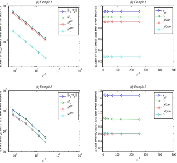
In Example 4.1, f is a periodic function. Therefore, it is natural to expect that the minorant Mper_⊖ (in which the periodicity is taken into account) will provide better results. In Example 4.2, the right-hand side is represented by a non-periodical function, and, therefore, we expect that Maper_⊖ will be better (at least for problems with relatively small amount of cells). The corresponding numerical results are depicted in Fig. 2 and confirm the proposed choice of the lower error bound. We note that in Example 4.1 the equality (2.25) holds and (cf. Remark 2.3) the majorant (4.2) coincides with the error. This fact is confirmed numerically (see Fig. 2 a, b). Example 4.2 shows that the majorant and minorants are quite sharp if the number of cells is sufficiently large (regardless of the condition (2.25)).

101 102 103 104 10−3

10−2

ε−1

Exact energy error and the error bounds

(a) Example 1 ||u_ε−w_ε1|| M + M₋per M₋aper 0 100 200 300 400 500 0.2 0.4 0.6 0.8 1 1.2 ε−1

Exact energy error and the error bounds

(b) Example 1 κ i₊eff i − eff,per i₋eff,aper 101 102 103 104 10−1 100 101 102 ε−1

Exact energy error and the error bounds

(c) Example 2 ||u_ε−w_ε1|| M + M₋per M₋aper 0 100 200 300 400 500 0.2 0.4 0.6 0.8 1 1.2 1.4 1.6 1.8 ε−1

Exact energy error and the error bounds

(d) Example 2 κ i₊eff i − eff,per i − eff,aper

Figure 2. Error bounds (left) and efficiency indices (right) for Example 4.1 and Example 4.2.

Example 4.3. Let d = 2 , Ω = (0, 1)2_{, and u}

ε∈ H1₀(Ω) be defined by the relation

∫

Ω

Aε∇uε⋅ ∇v = ∫ Ω

fv ∀ v ∈ H10(Ω) .

Here Aε is generated by the matrix ̂A := aI (cf. (1.4)), where

a :={_{ { a1> 0 in (0,1₂) 2 ∪ (1₂, 1)2 a2> 0 in (0, 1)2\ ((0,1₂) 2 ∪ (1₂, 1)2) . ̂ Π : a1 a1 a2 a2 (4.5)

Then (see, e.g., [14], pp. 35–39), A0= √a1a2. We choose

f = 2 √a1a2(x1(1 − x1) + x2(1 − x2))

such that

u0(x) = x1x2(1 − x1)(1 − x2). (4.6)

Exact solutions of the cell problems

∂ ∂yi( ̂ Aij(y) ∂Nk(y) ∂yj ) = ∂ ∂yi ̂_{Aik(y) in ̂Π = (0, 1)}2 Nkis periodic in ̂Π ⟨Nk⟩̂Π = 0 (4.7)

are found in [15] in the form

Nk(y) = ν (y + 1

2 ) + yk, k = 1, 2. (4.8)

Here ν(y) is the unique solution of the problem

− div (a ∇ν) = 0 in (−1, 1)2 (4.9)

with homogenous Dirichlet boundary conditions and a is defined by (4.5). This solution is given in polar coordinates (r, ϑ) centered at the origin by the relation

ν = r𝛾_{µ(ϑ) (4.10)} where µ(ϑ) := { { { { { { { { { { { { { cos(αβ) cos((ϑ − π₂+ α)𝛾), 0 ⩽ ϑ ⩽ π₂ cos(α𝛾) cos((ϑ − π + β)𝛾), π₂ ⩽ ϑ ⩽ π cos(αβ) cos((ϑ − π − α)𝛾), π ⩽ ϑ ⩽ 3π₂ cos((π₂− α)𝛾) cos((ϑ −3π₂ − β)𝛾), 3π₂ ⩽ ϑ ⩽ 2π (4.11)

is a continuous and piecewise smooth function and the numbers α, β, and 𝛾depend on a1/a2 and satisfy

the relations { { { { { { { { { { { { { { { { { { { { { { { { { { { { { { { a1 a2 = tan(β𝛾) cot(α𝛾) a2 a1 = − tan(α𝛾) cot(β𝛾) a1 a2 = − tan(β𝛾) cot(( π 2 − α)𝛾) a2 a1 = tan(( π 2 − α)𝛾) cot(β𝛾) 𝛾> 0 max{0, π𝛾− π} < 2α𝛾< min{π𝛾, π} max{0, π} < −2β𝛾< min{π, 2π}. (4.12)

It is known that ν has a restricted regularity (namely, ν ∈ H1+𝛾−ε_{(̂Π) for any ε > 0 ).}

We use this fact in order to verify the efficiency of the error majorant in different situations, we consider two cases, in which the ratio between a1 and a2 (and the regularity of Nk) are quite different.

∙ Case 1: let a1= 5.0, a2= 1.0. In this case, the solution (4.9) has 𝛾= 0.53544094560 and ϑ = π/2 (cf.

system (3.2) in [15]) so that ν ∈ H3/2_(Ω).

∙ Case 2: now, we set 𝛾= 0.1 and ϑ = π/2. By solving (4.11) and (4.12), we find that in this case a1 =

161.4476387975881 and a2 = 1.0. Here, ν ∈ H1+α(̂Π) with 0 < α < 0.1 , i.e., it is almost an H1

function.

To quantify the efficiency of the estimates (4.2 ) and (3.10), we compare them with the exact error

e := ‖∇(uε− w1ε)‖Aε. (4.13)

Since uε is unknown, we replace it by the ‘reference’ solution uref computed on a very fine mesh (h ≪ ε).

The corresponding efficiency indices are defined by the relations

ieff_⊕ = M⊕(w 1 ε; 0, 1, 1) ‖∇(uref− w1ε)‖Aε , ieff, per_⊖ = M per ⊖ (w1ε; 0) ‖∇(uref− w1ε)‖Aε . (4.14)

In Table 1 (Case 1) and 2 (Case 2), we present these quantities together with the quantity 𝜘 as in (4.3). We see that the estimates adequately reproduce the modeling error.

It is quite predictable that the estimates are better in the first case (related to a more regular ν ). For the first problem, efficiency indices of the majorant and minorant are quite close to 1. However, the estimates are also valid for the second case (minimal regularity). Indeed, the efficiency index of the majorant does not exceed 2.3 and the one of the minorant does not go below 0.7.

Table 1. Efficiency of error

majo-rant and minomajo-rant for Example 4.3, Case 1. ε−1 _ieff ⊕ ieff⊖ 𝜘 8 1.0714 0.8824 1.2141 16 1.0874 0.8781 1.2384 32 1.0988 0.8591 1.2790 64 1.1633 0.8461 1.3749

Table 2. Efficiency of error

majo-rant and minomajo-rant for Example 4.3, Case 2. ε−1 _ieff ⊕ ieff⊖ 𝜘 8 1.7024 0.8291 2.0533 16 1.9701 0.7961 2.4750 32 2.1848 0.7370 2.9644 64 2.2771 0.7124 3.1964

Acknowledgment: The authors are grateful to Swiss National Science Foundation for supporting this re-search under the grants 200021_119809 and 200020_134621. The first co-author also thanks the Institute for Mathematical Research (FIM, ETH, Zurich) for support. We are grateful to Dr. Christian Wüst — the finite ele-ment computations have been performed on the basis of his program JCFD.

References

[1] A. Abdulle, A. Nonnenmacher, A posteriori error analysis of the heterogeneous multiscale method for homogenization problems. C. R. Math. Acad. Sci. Paris,347 (2009), No. 17-18, 1081–1086.

[2] I. Babuška, W. C. Rheinboldt, A posteriori error estimates for the finite element method, Intern. J. Numer. Math. Engrg.,12

(1978), 1597–1615.

[3] I. Babuška, W. C. Rheinboldt, Error estimates for adaptive finite element computations, SIAM J. Numer. Anal.,15 (1978),

736–754.

[4] I. Babuška, I. Lee, C. Schwab, On the a posteriori estimation of the modeling error for the heat conduction in a plate and its use for adaptive hierarchical modeling, Appl. Numer. Math.,14 (1994), 5–21.

[5] I. Babuška, C. Schwab, A posteriori error estimation for hierarchic models of elliptic boundary value problems on thin domains, SIAM J. Numer. Anal.,33 (1996), 221–246.

[6] N. S. Bakhvalov, G. Panasenko, Homogenisation: Averaging Processes In Periodic Media: Mathematical Problems In The

Mechanics Of Composite Materials, Springer, 1989.

[7] A. Bensoussan, J.-L. Lions, G. Papanicolaou, Asymptotic Analysis for Periodic Structures, North-Holland, Amsterdam, 1978. [8] Z. Cai, S. Zhang, Recovery-based error estimator for interface problems: conforming linear elements, SIAM J. Numer. Anal.,

47 (2009), 2132–2156.

[9] M. Chipot, Elliptic Equations: An Introductory Course. Birkhäuser Verlag AG, 2009.

[10] D. Cioranescu, P. Donato, An Introduction To Homogenization, Oxford Lecture Series in Mathematics and its Applications, Vol. 17, Oxford University Press, 1999.

[11] A. Friedman, Partial Differential Equations, R. E. Krieger Pub. Co., Huntington, NY, 1976.

[12] P. Henning, M. Ohlberger, The heterogeneous multiscale finite element method for elliptic homogenization problems in perforated domains, Numer. Math.,113 (2009), No. 4, 601–629.

[13] P. Henning, M. Ohlberger, A-posteriori error estimation for a heterogeneous multiscale method for monotone operators

and beyond a periodic setting, Technical Report 01/11-N, FB 10, Universität Münster, 2011.

[14] V. V. Jikov, S. M. Kozlov, O. A. Oleinik, Homogenization of Differential Operators and Integral Functionals, Springer, Berlin, 1994.

[15] R. B. Kellogg, On the Poisson equation with intersecting interfaces, Appl. Anal.,4 (1975), 101–129.

[16] J. T. Oden, J. R. Cho, Adaptive hpq-finite element methods of hierarchical models for plate- and shell-like structures,

Com-put. Meth. Appl. Mech. Engrg.,136 (1996), 317–345.

[17] M. Ohlberger, A posteriori error estimates for the heterogeneous multiscale finite element method for elliptic homoge-nization problems, Multiscale Model. Simul.,4 (2005), No. 1, 88–114.

[18] L. E. Payne, H. F. Weinberger, An optimal Poincaré inequality for convex domains, Arch. Ration. Mech. Anal.,5 (1960), No. 1,

286–292.

[19] S. Repin, A posteriori error estimation for nonlinear variational problems by duality theory, Zapiski Nauch. Semin. (POMI),

243 (1997), 201–214.

[20] S. I. Repin, A posteriori error estimation for variational problems with uniformly convex functionals, Math. Comp.,69

(2000), 481–600.

[21] S. I. Repin, The estimates of the error of some two-dimensional models in the elasticity theory, J. Math. Sci., New York,106

[22] S. I. Repin, A posteriori estimates for partial differential equations, Walter de Gruyter, Berlin, 2008.

[23] S. I. Repin and T. S. Samrowski Estimates of dimension reduction errors for stationary reaction–diffusion problems,

Prob-lems of Math. Anal.,173 (2011), No. 6, 803–821.

[24] S. I. Repin, T. S. Samrowski, and S. A. Sauter, Combined a posteriori modelling–discretization error estimate for elliptic problems with variable coefficients, ESAIM, Math. Model. Numer. Anal.,46 (2012), No. 6, 1389–1405.

[25] S. I. Repin, T. S. Samrowski, and S. A. Sauter, A posteriori error majorants of the modeling errors for elliptic homogeniza-tion problems, C. R., Math., Acad. Sci. Paris,351 (2013), No. 23/24, 877–882.

[26] S. I. Repin, S. A. Sauter, and A. A. Smolianski, A posteriori error estimation for the Dirichlet problem with account of the error in the approximation of boundary conditions, Computing,70 (2003), 205–233.

[27] S. I. Repin, S. A. Sauter, and A. A. Smolianski, A posteriori estimation of dimension reduction errors for elliptic problems in thin domains, SIAM J. Numer. Anal.,42 (2004), No. 4, 1435–1451.

[28] T. S. Samrowski, Combined error estimates in the case of the dimension reduction, Preprint 16-2011, Universität Zürich, 2011.

[29] C. Schwab, A-posteriori modeling error estimation for hierarchic plate model, Numer. Math.,74 (1996), 221–259.

[30] Ch. Schwab, A. Matache, Generalized FEM for homogenization problems, in: Multiscale and multiresolution methods, Lect.

Notes Comput. Sci. Engrg.,20 (2002), 197–237. Springer, Berlin, 2002.