Co-channel digital signal separation : application and practice

Co-channel Digital Signal Separation:

and Practice

by

Dawei Shen

Application

Submitted to the Program in Media Arts and Sciences, School of

Architecture and Planning

in partial fulfillment of the requirements for the degree of

Master of Science in Media Arts and Sciences

at the

MASSACHUSETTS INSTITUTE OF TECHNOLOGY

February 2008

©

Massachusetts Institute of Technology 2008. All rights reserved.

Author ...

Program in Media Arts and Sciences

January 18, 2008

Certified by....

. . . . . . . . . . .... . .

Senior Rese rch Scientist

.... ... . . .

Andrew B. Lippman

of Me '

rts and Sciences

Thesis Supervisor

Accepted by..

MASSACHUSETS INSTTUTE OF TEOHNOLOGY

FEB 112008

LIBRARIES

Chai

...t . . . ... . . .. . . . . . . . . .

Deb Roy

rman, Departmental Comm' tee on Graduate Students

Co-channel Digital Signal Separation: Application and

Practice

by

Dawei Shen

Submitted to the Program in Media Arts and Sciences, School of Architecture and Planning

on January 18, 2008, in partial fulfillment of the requirements for the degree of

Master of Science in Media Arts and Sciences

Abstract

This thesis studies the theory and application of co-channel digital signal separation techniques. We set up a test-bed with the GNU Software Defined Radio (SDR) platform where we implement and experiment with single-antenna signal separation algorithms. We mainly investigate linearly-modulated digital signals. To do this, we design a multiple RFID card reader capable of decoding multiple commodity ID cards simultaneously. These passive RFID cards transmit DBPSK waveforms once activated. A signal separation function at the receiver delivers great convenience to the users without increasing the complexity and cost of the cards. Second, we derive the optimal criteria for deciding the start of an RFID frame. We show that the commonly utilized correlation rule is suboptimal and that a correction term needs to be considered to achieve the best detection performance. Several rules for frame synchronization are proposed and analyzed numerically using Monte Carlo simualtion. These signal separation techniques present an opportunity to improve the capacity of wireless systems and combat interference. This thesis documents design issues in the physical and application layers, thereby demonstrating the great flexibility and strength of the GNU SDR system.

Thesis Supervisor: Andrew B. Lippman

Co-channel Digital Signal Separation: Application

and Practice

Date of Submission: January 18, 2008

THESIS ADVISOR: Dr. Andrew B. Lippman

Senior Research Scientist of Media Arts and Sciences MIT lVgdia Lab

SIGNED:

THESIS READER: Dr. David P. Reed

Adjunct Professor of Media Arts and Sciences MIT Media Lab

SIGNED:

THESIS READER: Dr. Dina Katabi

Associate Professor of Electrical Engineering and Computer Science Computer Science and Artificial Intelligence Laboratory

Acknowledgments

Thanks to my advisors Andy and David for their ideas, guidance and support. Thanks to the incredible building - MIT E15. Since I came to the media lab, I have been deeply impressed and influenced by creative faculty members and students. Their ideas and demonstrations have inspired me to see how human-beings social lives may be combined with technology seamlessly. I feel so proud to be a member of this family.

Thanks to Dina for spending her time discussing with me, reading and comment-ing on my work.

Thanks to my parents and Liwen for their endless love and support.

Thanks to my labmates: Grace, Kwan, Hector, Pol, Nadav, Fulu and Sung for their help and encouragement. I am so fortunate to be working with you.

Thanks to all my friends!

Contents

1 Introduction 1.1 M otivation . . . . 1.2 Significance . . . . 1.3 Contributions . . . . 1.4 Structure ... ... 2 Background

2.1 Relevant Research Work . . . . 2.1.1 Algorithms for Linear Modulation Schemes . . . . 2.1.2 Algorithms for Constant Envelop Modulation Schemes 2.2 GNU Software Defined Radio . . . .

2.3 RFID System s . . . .

3 Design and Analysis of a Multiple RFID Card Reader 3.1 Specification of MIT ID Cards ...

3.2 Channel Model for Multiple RFID Signals ...

3.3 RFID Signal Separation ...

3.3.1 Maximum Likelihood (ML) Detection ...

3.3.2 Estimation of Power Levels . . . .

3.3.3 Calculating Amplitudes (gi) from Power Levels. .

3.3.4 Frequency Estimation and Phase Selection . . . .

3.3.5 Framing and Packetizing . . . .

21 . . . . 21 . . . . 25 . . . . 29 . . . . 29 . . . . 31 . . . . 35 . . . . 37 . . . . 40

3.3.6 Putting Everything Together . . . . 3.4 Sum m ary . . . . 4 Optimum Frame Synchronization

4.1 Introduction . . . . 4.2 The General MIMO Channel . . . .

4.3 The Multiple Access Channel . . . . .

4.3.1 The Frame-Synchronous Case 4.3.2 The Frame-Asynchronous Case 4.4 Summary . . . . 5 Future Research 6 Conclusions A Amplitude Estimation 43 . . . . 43 . . . . 44 . . . . 48 . . . . 49 . . . . 53 . . . . 69

List of Figures

1-1 A cocktail party versus a communication network, where a receiver is

not capable of decoding simultaneously transmitted signals . . . . 12 1-2 A simplified channel model of digital signal separation. Two

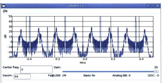
transmit-ters are sending signals to the same receiver at the same time. . . . . 13 3-1 The spectrum of the received signal r(t) displayed using the Software

Spectrum Analyzer provided by GNU Radio, one card is present,

f,

=

500kHz... ... 23

3-2 The spectrum of ro(t), the output signal of the band-pass filter,

cen-tered at fo =62.5kHz, f,=500kHz . . . . 24

3-3 The spectrum of po(t) = 1/4B(t) (left) and its time domain waveform

(right), only one card is activated, f,=500kHz . . . . 25

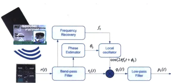
3-4 The diagram of the modules that pre-process the RFID signal before the separation function block, which is implemented using GNU Radio 27 3-5 Each symbol is expanded into 32 identical symbols that are consecutive

in tim e. . . . . 28 3-6 The time-domain baseband discrete signal generated by two RFID

cards (r[m]), sampled at

f,

=500kHz, down-converted from 62.5kHz band to 0-band . . . . 29

3-7 The histogram of the discrete samples (r2[m]) generated by two RFID

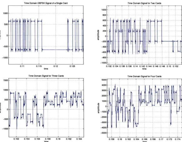
3-8 The time domain baseband signals generated by one, two, three and

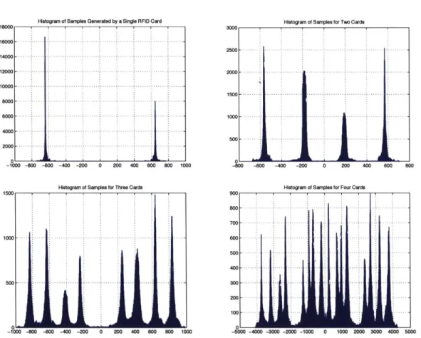
four RFID cards, from which we can see 2, 4, 8 and 16 power levels respectively. . . . . 33 3-9 The histogram of the discrete samples generated by one, two, three and

four RFID cards, from which we can see 2, 4, 8 and 16 power levels respectively . . . . 34

3-10 The spectrum of the mixed signal qo(t) (above) and the histogram of

the samples of the baseband signal (r2 [M]) generated by two cards

(bottom), with 0o = 0, F/4, w/2, 3w/4 . . . . 38 3-11 The spectrum of the mixed signal qo(t) (above) and the histogram of

the samples of the baseband signal (r3

[m])

generated by three cards

(bottom), with 00 = 0, ir/4, r/2, 37r/4 . . . . 39 3-12 The complete block diagram of the multiple RFID cards' reader,

im-plemented using GNU Radio . . . . 41

3-13 The graphical user interface of the multiple RFID cards' reader, built

using PyGT K . . . . 41 4-1 The comparison between the correlation rule and the optimal decision

rule for frame detection in the frame-synchronous case. Two transmit-ters use Barker codes, hi = 1, h2 = 0.8, noise variance (o.

2_{) ranges} from 0.5 to 9.5 . . . . 51

4-2 The comparison between the correlation rule and the optimal decision rule for frame detection in the frame-synchronous case. Two transmit-ters use Barker codes, hi = 1, h₂ = 0.5, noise variance (o.2) ranges

from 0.5 to 9.5 . . . . 51

4-3 The comparison between the correlation rule and the optimal decision rule for frame detection in the frame-synchronous case. Two transmit-ters use Barker codes, hi = 1, h₂ = 0.2, noise variance (o.2) ranges from 0.5 to 9.5 . . . . 52

4-4 The comparison between the correlation rule and the optimal decision rule for frame detection in the frame-synchronous case. Two trans-mitters use random sync-words, hi = 1, h2= 0.5, noise variance (a2)

ranges from 0.5 to 9.5 . . . . 52

4-5 The comparison between the correlation rule and the optimal decision rule for frame detection in the frame-synchronous case. Three trans-mitters use Barker codes, hi = 1, h2 = 0.6,h3 = 0.3, noise variance

(a2_{) ranges from 0.5 to 9.5 . . . .} 53

4-6 Separate frame detection using the correlation rule, the optimal deci-sion rule and the suboptimal rule using Gaussian approximation in the frame-asynchronous case. Two transmitters use Barker codes, hi = 1, h2= 0.5, and noise variance (a2_{) ranges from 0.5 to 9.5 . . . . 65}

4-7 Separate frame detection using the correlation rule, the optimal deci-sion rule and the suboptimal rule using Gaussian approximation in the frame-asynchronous case. Two transmitters use Barker codes, hi = 1,

h2 = 1, and noise variance (a2) ranges from 0.5 to 9.5 . . . . 65

4-8 Separate frame detection of transmitter 2's signal using the correlation rule, the optimal decision rule and the suboptimal rule using Gaussian approximation in the frame-asynchronous case. Two transmitters use Barker codes, hi = 1, h2 = 0.75, and noise variance (a2) ranges from

0.5 to 9.5 . . . . 66

4-9 Separate frame detection of transmitter 2's signal using the correlation rule, the optimal decision rule and the suboptimal rule using Gaussian approximation in the frame-asynchronous case. Two transmitters use Barker codes, hi = 1, h2 = 0.5, and noise variance (a2) ranges from

4-10 Separate frame detection of transmitter 2's signal using the correlation rule, the optimal decision rule and the suboptimal rule using Gaussian approximation in the frame-asynchronous case. Transmitter 1 uses the Barker code, transmitter 2 uses the Neuman-Hofman code. hi = 1,

h2= 0.5, and noise variance (o.2) ranges from 0.5 to 9.5 . . . . 68

4-11 Separate frame detection using the correlation rule, the optimal de-cision rule and the suboptimal rule using Gaussian approximation in the frame-asynchronous case. Three transmitters use Barker codes,

hi = 1, h2 = 0.5, h3 = 0.3, and noise variance (o.2) ranges from 0.5 to 9.5 69

4-12 Joint frame detection of both transmitters' signals using the optimal decision rule. Transmitter 1 uses the Barker code, transmitter 2 uses the Neuman-Hofman code. hi = 1, h₂ = 0.75, and noise variance (o.2) ranges from 0.5 to 9.5 . . . . 70

5-1 The block diagram of the GMSK transmitter . . . . 72

Chapter 1

Introduction

1.1

Motivation

The cocktail party effect describes the human's exceptional ability to listen to a single speaker among a mixture of conversations and background noises [3]. In a very noisy party, we can still listen and understand what our friend says while simultaneously ignoring what nearby people are saying. If another friend far away suddenly calls our names, we can still recognize the sound and respond quickly. Interestingly, engineers have not developed communication devices with such amazing auditory capabilities. Figure.1-1 compares these two scenarios.

Consider the case of having multiple RFID cards coexisting in our wallet. In order to open a door protected by an RFID reader, we usually have to flip the wallet for several times in front of the reader or even take the correct card out. All the cards transmit RF signals interfering with each other. However, the reader only responds to the loudest one or simply chooses to stay confused. A more sophisticated system bypasses this problem by avoiding simultaneous transmissions by using smarter, but more costly RFID cards. An immediate question is: why don't we enable the receiver to separate and decode multiple signals, so that the other parts of the system remain

Cocktail Party Effects in a wireless network, no

(fron Larryeodine.com) simultaneous transmissions

Figure 1-1 - A cocktail party versus a communication network, where a

re-ceiver is not capable of decoding simultaneously transmitted signals

In a wireless network system, if multiple signals coexist in the same channel, undesired signals are considered as interference to the primary signal. Therefore, communication devices must be regulated to share the channel. The current solution generally adopts time-division multiplexing (TDM), frequency-division multiplexing (FDM) or code-division multiplexing (CDM). The multiplexing divides the channel into several orthogonal logical channels. Such practice requires precise coordina-tion and timing synchronizacoordina-tion. In a random access network such as today's Wi-Fi networks, simultaneously transmitted packets lead to a collision. Both packets are discarded and retransmissions must be made later. Intuitively, a considerable amount of information is abandoned and wasted in conventional network settings. If sophis-ticated signal processing could enable us to jointly decode concurrently transmitted signals with high reliability, it is expected that the capacity of wireless networks can be effectively improved and higher layer protocols can be optimally redesigned.

1.2

Significance

Digital signal separation has wide applications in cellular networks and RFID systems which are presented in this thesis. More importantly, it provides us with a new perspective on the design and analysis of future ad-hoc network systems, and leads us to rethink how we deal with interference.

TX Antenna

Figure 1-2 - A simplified channel model of digital signal separation. Two

transmitters are sending signals to the same receiver at the same time.

In cellular networks, the dominant channel impairment is co-channel interference (CCI), introduced by frequency reusage. Advanced signal processing techniques can be applied to the receiver to mitigate the effects caused by the interfering signals and noise. In today's Wi-Fi networks, the medium access control (MAC) layer as-sumes simple collision models, i.e., collisions among users mainly cause the failure of packet delivery. The basic approach to improve the MAC's performance is to resolve collisions by limiting transmissions. Conventional MAC protocols, especially for ran-dom access ad-hoc networks, suffer from hidden terminal problems, which severely limit the effectiveness of techniques based on carrier sensing. Digital signal separa-tion apparently provides an alternative way to solve the hidden terminal problem. Furthermore, if the receiver has the multipacket reception capability, the MAC layer protocol should encourage, rather than limit, simultaneous transmissions of users to improve the throughput of the network[18].

In this thesis, we study the theory and application of co-channel digital signal separation techniques. We set up a test-bed with the GNU Software Defined Radio

(GNU SDR, or GNU Radio) platform, on which we implement and experiment with

single-antenna signal separation algorithms.

First, we design a multiple RFID cards' reader, which is capable of reading and decoding multiple MIT student ID cards simultaneously. These passive RFID cards transmit DBPSK waveforms once they get activated. By enabling signal separation capability at the receiver, we deliver great convenience and efficiency to the users without increasing the complexity and cost of the cards.

Second, We derive the optimal criteria for deciding the start of an RFID frame, commonly known as the optimum frame synchronization problem, for multiple access channels. Due to its important theoretical value, we devote a standalone chapter to this topic.

We document design issues we have encountered in physical and application layers, thereby demonstrating the great flexibility and strength of the GNU Radio system. Data will be processed online and offline in GNU Radio to analyze the effects and evaluate the performance.

1.3

Contributions

The main contributions of the work discussed in this thesis include:

1. We implement a complete multiple RFID card reader, capable of decoding

sig-nals emitted by simultaneously activated RFID tags. Compared with the pre-vious work on multiple RFID decoding presented in [20], our work exhibits significant improvements in many aspects:

" Our extendible algorithm is capable of reading more cards than the method

introduced in [20], which handles only two cards. The design and anal-ysis presented in this thesis is mostly based on four cards. However, the number of cards that can be successfully decoded is only constrained by the computational power and the amount of memory used in the software radio system, not the algorithm itself.

" The reader we implement runs in real time and delivers the identity

infor-mation embedded in the cards with little processing delay.

* We estimate the power levels of the received signal by using a histogram of the received samples, and then calculate the amplitudes of the transmitted signals by solving a set of linear equations according to the least square error criteria. This approach provides very accurate estimates of the signal

amplitudes. In contrast, [20] uses a simple approach to estimate signal amplitudes, which usually leads to incorrect detection due to its inaccuracy. Additionally, the approach used in [20] can not be extended.

2. We study the problem of optimum frame synchronization for multiple access channels (MAC). While Massey [15] and several following researchers have dis-covered the optimal criteria for frame detection in point-to-point channels, few research efforts have been made for multiple access channels, especially for the frame-asynchronous case. In this thesis, we present new research results for both frame-synchronous and frame-asynchronous cases. We show that the opti-mal rule for frame detection in multiple access channels adds a correction term to the correlation term. When multiple transmitters are present, Gaussian

ap-proximation can be used to simplify the decoding rule.

1.4

Structure

In the next chapter, we summarize the relevant background materials on co-channel digital signal separation. We will survey existing algorithms and discuss their us-abilities. We also introduce the fundamental principles of the GNU Radio platform and the RFID system. Chapter 3 documents a detailed process of designing a multi-ple RFID card reader. We discuss design decisions and present numerical results in this chapter. The optimum frame synchronization algorithm for locating the starting sample of an RFID frame is derived in Chapter 4. We demonstrate that the optimum decision rule we develop outperforms the simple correlation rule we used to utilize. We introduce our future research on signal separation algorithms for GMSK modula-tion in Chapter 5 for both synchronous and asynchronous cases. Finally, in Chapter

Chapter 2

Background

2.1

Relevant Research Work

Co-channel signal separation techniques have been developed by researchers mainly as tools to alleviate co-channel interference (CCI) encountered in cellular networks and other communication systems. Many proposed algorithms stem from interfer-ence cancellation/suppression techniques and adaptive equalizing methods. Though tremendous research efforts have been focused on utilizing antenna arrays instead of one single receive antenna, multiple antennas usually lead to costly and complex receivers with unacceptable sizes. Therefore, a single antenna system is an attractive option, which is also the focus of this thesis.

Generally speaking, digital waveforms employed today can be categorized into two classes according to their different modulation schemes: linear modulation (MPSK/QAM, e.g.) and constant envelop modulation (GMSK/MSK, e.g.)[2]. In linear modulation, a symbol is mapped to a complex point of a constellion on a 2-dimensional plane. These complex symbols then pass through a pulse-shaping function block, which, coupled with a match filter at the receiver, is designed to relieve symbol inter-ference (ISI) effects caused by the wireless channel. The impact of the channel on the signal is usually modelled as an FIR filter with complex-valued taps or the so-called

channel coefficients. With regard to constant envelop modulation, the amplitude of a sample at any time instant is unvarying. The digital information is embraced inside the phase, or more precisely, the instantaneous frequency of the signal. Over the past decade, various co-channel signal separation methods have been proposed for different modulation schemes under different assumptions.

2.1.1

Algorithms for Linear Modulation Schemes

For linear modulation schemes, a series of nonlinear methods based on joint maximum likelihood sequence estimation (JMLSE) were proposed in [7, 5, 6]. These literatures have an in-depth and thorough treatment of the optimal joint estimator of two co-channel linearly modulated signals. In [7], a suboptimal, joint MAP symbol detection

(JMAPSD) algorithm based on a Bayesian recursion was proposed. Good estimates

of the primary and secondary signal powers are assumed to be available a-priori. The channel coefficients are assumed to be known for both JMLSE and JMAPSD. Alter-natively, they can be estimated blindly, which leads to joint blind MAP co-channel symbol detector (JBMAPSD). Besides Giridhar's outstanding work, a conventional independent component analysis (ICA) approach to blindly separate MPSK signals is described in [19]. A quasi-linear demod-remod system for recovering co-channel QAM signals in the presence of ISI was proposed in [9]. Accurate estimation of channel co-efficients plays a crucial role and the study in [10] addresses a pilot-based MMSE technique for multiuser channel estimation in a TDMA system.

2.1.2

Algorithms for Constant Envelop Modulation Schemes

For constant envelop modulation such as GMSK, the demod-remod technique is an attractive option for its conceptual simplicity and low design complexity [8]. Algo-rithms based upon JMLSE were discussed and analyzed in [16, 17]. Both papers assume GMSK signals must be transmitted synchronously. If we treat continuous-phase frequency shift keying (CPFSK) signals as ordinary FM signals, then techniques

for analog FM signal separation could also be brought into the picture. Hamkins compared three approaches in his work: cross-coupled phase locked loop (CCPLL) method, joint Viterbi algorithm, and an analytic technique [11], which we will study and test extensively in the thesis. All three methods are built upon the same idea: jointly tracking the phases of the two waveforms since the digital information is car-ried in the instantaneous frequencies of the signals. This is an effective approach because it doesn't require symbol-level synchronization between the two sources and the knowledge of training sequences is not necessary at the receiver. Besides, this method is robust to carrier frequency offsets. However, we have to transmit packets continuously from the two sources to make them behave like analog FM signals. In [12], the joint estimation problem is formulated using state space equations and the estimator structure is derived based on the extended Kalman filter (EKF).

2.2

GNU Software Defined Radio

Most algorithms introduced above have been only validated via mathematical proofs or computer simulation. Few of them provide convincing results for real-world, over-the-air data. Most importantly, some methods are developed based on assumptions which are hardly realizable in practice or usable with existing hardware. For example, some methods require accurate estimation of channel coefficients and signal power, while some methods rely on the synchronization of two packets. We usually meet unexpected obstacles and challenges when we implement these ideas in real systems

and test the algorithms using data that come through a real wireless channel.

GNU Software Defined Radio, together with its hardware counterpart, the

Uni-versal Software Radio Peripheral (USRP) board, provides an ideal test-bed for ex-perimenting with these new techniques. 'GNU Radio is a free software toolkit for learning about, building, and deploying software defined radios'. GNU Radio takes what is traditionally done in hardware and brings it into software, providing great convenience and flexibility for academic users. Reconfigurability is the key feature[4].

The USRP board is the associated hardware counterpart specifically designed

by Ettus for GNU Radio use[1]. The USRP main board contains four 64 MS/s

12-bit analog-to-digital converters(ADC), and four 128 MS/s 14-bit digital-to-analog converters (DAC). The USRP board exchanges samples with the computer via a high-speed USB 2.0 interface. Due to the limitation of the USB bus, the USRP is only capable of processing signals with bandwidths of up to 16 MHz. Various daughter boards are available covering various frequency bands between 0 and 2.9 GHz.

At this stage, we have a stable functional DBPSK, GMSK and OFDM imple-mented and carefully tested in the GNU Radio code base. Despite certain limitations imposed by the current architecture of GNU Radio, we can readily build our signal separation program based on the existing signal processing modules. One shortcom-ing is that GNU Radio doesn't support feedback flows from one block back to another block.

2.3

RFID Systems

Radio frequency identification (RFID) is an automatic identification method using devices including RFID tags and readers. An RFID tag contains an antenna for receiving and transmitting signals, and an integrated circuit for storing and processing identification information. RFID tags can be roughly categorized into two types. Passive tags do not have internal power supply, i.e., the interal circuit can only be activated by incoming radio frequency signals. In contrast, active RFID tags have their own power sources and broadcast RF waves to readers. RFID systems work in different frequency bands: low frequency (LF, 125kHz), high frequency (HF, 13.56MHz) and ultra high frequency (UHF, 900MHz).

RFID technology has received remarkable attention in recent years. It has very broad applications in transportation payments, inventory control, product tracking, and people/animal identification. At the same time, it also has engendered consider-able controversy on privacy concerns.

MIT deploys an RFID system on campus using Indala's products. All student ID cards are passive RFID tags working in the 125kHz band. If multiple ID cards appear in front of the reader, all of them will accumulate enough power from the carrier signal emitted by the reader, and start to transmit signals back to the reader. In such a situation, the reader may not be able to decode the desired identification signal. This motivates us to investigate signal separation methods to solve this problem.

Chapter 3

Design and Analysis of a Multiple

RFID Card Reader

In this chapter, we present a complete system design of a multiple RFID card reader, which is implemented using the GNU Software Radio system. The reader is capable of decoding simultaneous RFID signals. We first introduce the basics of the RFID system deployed at MIT. Then, we model multiple RFID signals mathematically and formulate the separation problem as a maximum likelihood (ML) detection problem. We next describe the algorithm for estimating the power levels of the received signal and calculating the signal amplitudes from the estimated levels. Design parameters and their impacts on the decoding performance are then analyzed numerically. We demonstrate that the signal separation function at the receiver delivers great

conve-nience to the users without increasing the complexity and cost of the cards.

3.1

Specification of MIT ID Cards

In this section, we introduce the basics of the MIT RFID card system that we work with. MIT deploys Indala Proximity 125kHz readers and compatible student ID cards on campus. The readers constantly generate 125kHz sine waves. When a

passive student RFID card approaches the reader, it gets activated after accumulating enough power. On the receiving end, the reader sees the 125 kHz carrier gets AM modulated by a 62.5 kHz signal. The bits are DBPSK encoded on the 62.5 kHz signal.

A '1' corresponds to a phase shift and a '0' means no phase shift. Mathematically, the

digital signal received by the reader when only one card is activated can be represented

by

r(t) = (A + B(t) cos(2w62.5kt + #)) cos(27r125kt + 0). (3.1) A is the amplitude of the 125kHz carrier when no card is present. 0,

#

are unknown, but correlated phase offsets. They satisfy the relationship:

0-2#=0 or±ir, (3.2)

because the RFID card derives its clock from the external sine wave. All the RFID cards transmit signals that are synchronized with the carrier, with possible 0, ±r/2, 7r

ambiguities. B(t), generated by the passive RFID card, is a None-Return-to-Zero (NRZ) DBPSK waveform containing the encoded binary information. Its time domain waveform is shown in Figure.3-3. B(t) can be expressed by

B(t) = h ( dka(t - kT), (3.3)

k

where h is the amplitude representing the signal strength, a(t) is a simple on-off square wave with a level of 1 when 0 < t < T, and 0 elsewhere, dk is a series of binary symbols valued from 1, -1, differentially encoded. T is the symbol period. The symbol rate is

f,

= 125e3/32kHz e 3.91kHz. T = 1/f, r 2.56. 1-04 s.

Figure.3-1 shows the spectrum of the received signal r(t) when an RFID tag is activated. Though the signal is expressed using continuous-time representation in

Eq.(3.1) and Eq.(3.3), we process the signal discretely by first sampling the signal.

The sampling rate we use is

f,

= 500kHz. The strong peak at 125kHz is the carrier signal emitted by the reader. The two distinct lobes beside the peak, centered around

3

2C

-2 'M

ILIL

I

-0.4 -0.2 0.0 0.2 0.4

MHz

Center freq: 0 Gain: 20 Decim: 64 Fs@USB: 1M Basic Rx Analog BB: 0 DDC: -0

Figure 3-1 - The spectrum of the received signal r(t) displayed using the

Software Spectrum Analyzer provided by GNU Radio, one card is present,

f, = 500kHz

62.5kHz and 187.5kHz, exhibit the digital signals generated by the RFID tags. This can be explained by expanding r(t) into three terms,

1 r(t) = -B(t) cos(27r62.5kt +# -9) 2 1 +A -cos(27rl25kt + 9) + -B(t) cos(27r187.5kt + # + 0). (3.4) 2

Note that there are higher order harmonics visible in the spectrum, which are generated from the reader's circuitry. By using a band-pass FIR filter with cut-off frequencies of 20kHz and 105kHz, we remove the last two high frequency terms, retaining the information in B(t),

1

ro(t) = -B(t) cos(27rfot +

4o).

(3.5)

2

We can further decode the binary symbols from ro(t). The use of a band-pass filter guarantees that the DC component will also get removed. The spectrum of the resulting filtered signal is shown in Figure.3-2. The nominal value of fo is 62.5kHz. However, due to hardware limitation, there is usually a small frequency offset, which

X1o Spectrum of RFID tags signal 18 -. . 16- 14-08 -06 . 04 -02 - . 0 1.5 -1 -0.5 0 0.5 1 1.5 frequency _{x 10}

Figure 3-2 - _{The spectrum of ro(t), the output signal of the band-pass filter,}

centered at fo =62.5kHz, f,=500kHz

must be estimated accurately. 0 =

#

- 0.

After recovering the carrier, B(t) can be obtained by multiplying ro(t) with a cosine wave cos(27rfot +

#o)

that is locally generated (mixing). Then, we can low-pass filter the multiplied signal. This process is also called digital down conversion because the spectrum of the signal is moved from 62.5kHz down to OHz. Mathematically,

qo(t) = ro(t) cos(27rfot +

#

0) 1 1

= B(t) + -B(t) cos(4irfot + #o)

po(t) = -B(t). (3.6)

4

Finally, we obtain a square-shaped signal, po(t) = B(t), with which we can directly decide digital information, as shown in Figure.3-3.

All the equations above use continuous-time representations. In a digital system,

all signals are sampled by the analog-to-digital converter (ADC), and processed in the discrete domain. We set up the USRP board with a sampling rate of

f,

= 500kHz. The symbol rate of the RFID signal is

fsy

m = 125/32kHz. Therefore, the oversampling rate for each symbol is

f/fy

m = 128. Each MIT ID is uniquely identified with 224

1.8 - ---1000 - -- -1 .6 -- - -- -. .-. -. . . 1,2 - - -. -. -..-

-0.6

-.-.-.-.-

-

.-

.--

-500

-.-.-.

--.-.-.-0.4-+ 0.2 + + - - - - -1000 - --...- -..-- - - ... -5 -4 -3 -2 -1 0 1 2 3 4 5 0.11 0.115 0.12 0.125

Ire ncy X104 lime

Figure 3-3 - The spectrum of po(t) = 1/4B(t) (left) and its time domain

waveform (right), only one card is activated, f.=500kHz

bits, which we call a frame. Each frame starts with 30 zeros, which we can clearly observe from Figure.3-3. The RFID card, once activated, repeatly transmits the 224 bits over and over again. Interestingly, out of these 224 bits, only 32 vary among cards, all the other bits remain constant. This fact implies we can have as many as

192 bits as the sync-word when we try to locate an RFID frame. This important fact

also helps us decode the information more reliably.

3.2

Channel Model for Multiple RFID Signals

When multiple cards come close to the reader, all of them may get activated and start transmitting signals back to the reader. There are several important facts we must be aware of in our system design.

First, cards usually get activated and start to transmit frames at different starting time instants. The timing offset between two signals must be a multiple of (1/125k)

seconds (one period of the carrier). This is because RFID tags synthesize their in-ternal clocks from the incoming 125kHz carrier, thus they transmit signals that are synchronized with the 125kHz sine wave. Second, because of the various distances between the cards and the reader, and also because of the nuances in hardware man-ufacturing, the signal strengths can be significantly different. This is a crucial factor

in being able to separate signals. Finally, all signals have the same center frequency

fo, but different phases

do,

as shown in Eq.3.5. As introduced above, there can be a

7r or 7r/2 ambiguity between signals. This is another important factor in our system design. We will examine the effects of the phase offsets more carefully later.

The analysis above gives us the continuous-time channel model for multiple RFID signals:

N

ro(t) =

3

Bl(t - Ti) cos(27rfot + #o + 01) + n(t). (3.7)

This channel model assumes the signal has been processed with the band-pass filter, but without down converting. Note that we still use ro(t), the same notation we used in Eq.(3.5), to denote the output signal of the band-pass filter. n(t) is the additive white Gaussian noise. N is the number of activated cards.

#o

is the unknown phase offset, as shown in Eq.(3.5). 01 represents the phase ambiguity, which takes on values

from 0, ±7r/2, 7r. r is the timing offset, which is a multiple of (1/125k) seconds .Bi(t)

has been given in Eq.(3.3), with the index 1.

Bi(t) = hi E dk,Ia(t - kT). (3.8)

k

Figure.3-4 shows the block diagram of all pre-processing modules that process the received signal before we can apply the separation algorithm.

Because of the variance of the phase offsets among different signals, we cannot recover the phases of these signals using any conventional carrier synchronization approaches. In fact, the effects of the phase offsets can be reflected in the amplitudes after we down-convert the signal to 0-band. Remember that we down-convert a signal by low-pass filtering the mixing of ro(t) and a locally generated cosine wave.

Figure 3-4 - The diagram of the modules that pre-process the RFID signal before the separation function block, which is implemented using GNU Radio Mathematically, the output of the mixer is

qo(t) = ro(t) cos(27rfot + Go)

N

= ( BI(t - Tj) cos(27rfot + $o + 01) cos(2irfot + 0o) N

= ( Bi(t- 1) cos($o +01 -o)

1=1

N

+ Y( B(t - ri) cos(47rfot + $o + 01 + 00), (3.9)

1=1

where cos(27rfot + 9o) is the cosine wave we generate locally. fo must be estimated accurately using frequency recovery techniques. 0o is only a design choice for us, and is not a parameter recovered from the received signal. We will discuss the selection

of 00 in detail later. Note that here, we omit the noise term n(t) for clarity. After

low-pass filtering, we obtain: IN

Po(t) = Bi(t - ) cos(4o + 01 - 6o). (3.10)

fac-01001011-..

00.. -011.. 100 -.. 000- 011-.. 100 --011 .11-.. l.-...

32 O's 32 I's 32 O's 32 O's 32 l's 32 O's 32 l's 32 I's

Figure 3-5 - Each symbol is expanded into 32 identical symbols that are

consecutive in time.

tor of B(t), which can be incorporated into the amplitudes h, inside Bl(t), i.e.

g, = 1/2h, cos(<o + 01 - 00). Each B, (t) is a square-shaped signal as shown in

Figure.3-3. , must be multiples of (1/125k) seconds, which provides us with some degree of

convenience. If each (1/125k) second is a unit time, the starting time of each RFID signal must be aligned with one of these units. The symbol rate of the DBPSK signal is (125/32)kHz. We can split each symbol in time and treat it as 32 identical symbols.

By doing this expansion, we achieve a higher symbol rate of 125kHz. More

impor-tantly, we achieve symbol level synchronization. Figure.3-5 explains this expansion.

The analysis above leads to a very succinct expression for the corresponding discrete-time channel model for multiple signals,

N

r[m] = gi - di[m] + n[m]. (3.11)

1

The a(t) in Eq.(3.3) disappears in the equation since it only takes value from 0 or 1. g, is the amplitude we calculated in the continuous-time channel model before. Here, we would like to incorporate the effects caused by different phase offsets. dl[m]'s are ±1 symbols. m here indexes the discrete samples. It has valid meanings in both 'sampling rate (500kHz)' indexes and 'expanded symbol rate (125kHz)' indexes. The difference

is an oversampling factor of fs/fesym = 4. Since we are working with sampling-rate

discrete signals, we assume m indexes the signal with the sampling rate. Note that in this case, each ±1 symbol in the original packet is expanded into 128 samples.

Time Domaln Signal for Two Cards

0.132 0.134 0.136 0.138 0.14 0.142 0.144 0.146 0.148 0.15 0.152 time

Figure 3-6 - The time-domain baseband discrete signal generated by two RFID cards (r[m]), sampled at

f,

=500kHz, down-converted from 62.5kHz band to 0-band

Hence, the RFID signal separation problem can be summarized as: given r[m], how can we decode dk,I's in Eq.(3.8) reliably?

3.3

RFID Signal Separation

3.3.1

Maximum Likelihood (ML) Detection

Let's consider the simplest case when only two cards are activated simultaneously. After band-pass filtering the signal, we obtain an accurate estimate of fo from ro(t)

by using frequency recovery. With an appropriately chosen phase 0, we create a local

cosine wave and mix it with the signal. Then, we obtain r[m] by low-pass filtering the output of the mixer, whose time-domain waveform is displayed in Figure.3-6.

Compared with Figure.3-3, where only two power levels are present, Figure.3-6 demonstrates four different levels. We can understand this phenomenon from the

discrete channel model

r2[M] = gi -di[m]

+

92 -d2m]

+

n[m]. (3.12)

The subscript 2 is used to indicate the number of active signals. Without considering the noise term n[m] and the Gibbs phenomenon caused by FIR filtering effects, there should be four different power levels existing if gi and g2 are different, i.e.: g1+92, gi

-92, -9i + 92, -gi - 92. Without loss of generality, we assume 9i > g2 > 0. This is

clearly observable from Figure.3-6, where all samples are valued around ±600, ±200.

If we have estimated these four levels accurately (assuming they are 12, l₁, -11, -12

and 12 > 1i > 0), we can further derive the values of 9i, 92 into gi = (12 + li)/2 and

92 = (12 - li)/2. The probability density function (pdf) of r2[m], given that n[m] is

white Gaussian noise is thus

1 (r21m]-g, dj[Ilm-gr.d2[m])2

Pr2 [M] (r2 [in]) - e 2o,, (3.13)

where o.2 is the variance of the Gaussian noise.

Maximum likelihood (ML) detection is to find a pair (di[m], d2[m]) from the four

possible combinations, (1,1), (1,-1), (-1,1) and (-1,-i), such that the pdf in Eq.(3.13) is maximized. Equivalently, the distance between the received sample and the power level produced by (d1[in], d2 [M])

|r2[m] - gi - di[m] - g- d2[m]| (3.14)

is minimized. In other words, we choose a pair that gives us a power level that is closest to r2

[m].

To further simplify the decision making process, we notice that

the whole set of real numbers can be divided into four decision regions, which are separated by three thresholds: gi, 0 and -gi. We choose (di[m], d2[m]) to be (1,1)

if r2[m] > 91, (1,-1) if 0 < r2[m] < 9i, (-1,1) if -91 < r2[m]

<

0, and (-1,-i) if

The ML detection algorithm above presumes accurate estimates of the power levels, i.e., gi and 92, are available. We will explore the estimation algorithm in subsequent subsections. Note that the ML detection algorithm can be easily extended to cases when more RFID cards' signals are present. For example, for the three cards' cases, the discrete channel model becomes

r3[m] - gi -di[m] + g2 -d2[m] + g3-d3[n] + n[m). (3.15)

In this case, there are eight possible power levels:gi

+

g2 + g3, g1 + g2 - 93, gi - 92 + 93,gi -- g2 - g3, -g1 + g2 + g3 , -gi + g2 - 93, -gi - 92 + g3, -g1 - - 93. The ML

detection rule is comparing r3[m] with seven thresholds and making a choice out of

the eight possible states.

3.3.2

Estimation of Power Levels

In this subsection, we discuss how to estimate the distinct power levels. We are motivated by the fact that the power levels can be easily read from the probability density function(pdf) of the received samples. The location of the peaks (local max-ima) are believed to be good estimates of the power levels. In our system design, we try to approximate the distribution by using a histogram of the samples, as shown in Figure.3-7.

In order to create the histogram, we divide the range of possible sample values into 1000 small bins and count the number of samples that fall into each bin. After obtaining the histogram, we perform peak detection in the histogram. By finding the local maxima, we locate where the signal power levels are. Finding these peaks can be done efficiently, we require that the number of samples in a bin must exceed a certain threshold and it must be larger than the counts for nearby bins.

We should emphasize that this approach of estimating the power levels is a good demonstration of the strength and flexibility provided by GNU Software Radio. In order to create the histogram of the samples, we need to buffer a large amount of

Histogram of Samples for Two Cards

Figure 3-7 - The histogram of the discrete samples (r2[m]) generated by two

RFID cards, f,=500kHz

data. The histogram in Figure.3-7 results from a collection of 200,000 samples. The requirement for a large amount of memory space is too demanding to be satisfied

with most hardware implementation. However, software radio takes advantage of the convenience of software programming and the ease of memory allocation, making realization of our algorithm much simpler.

All peaks should be detected symmetrically, i.e., if 1k is the position of a peak

representing a power level, - 1_{k should be one too. This one degree of redundancy}

helps the peak detection become more robust.

In Figure.3-8 and Figure.3-9, we compare the time-domain waveforms and the histgrams of the samples for one, two, three and four card cases. The ML detection and power level estimation algorithms apply in the same way for the three and four card cases. For three cards, we can observe eight different signal levels, while four cards make 16 levels visible. Again, we emphasize that all peaks are symmetric. When we do peak detection, we must take this symmetry into account and choose from unwanted noisy peaks. For example, the peak detection in the four card case is

Time Domain DBPSK Signal of a Single Card

time

Time Domain Signal for Two Cards

j

..

L

J- i

- T

132 0.134 0.136 0.138 0.14 0.142 0144 0.146 0.148 0.15 0.152

time

Time Domain Signal for Four Cards

0.158 0.18 0.162 0.164 0.166 0.168 0.17

im

0.172 0.174

Figure 3-8 - The time domain baseband signals generated by one, two, three and four RFID cards, from which we can see 2, 4, 8 and 16 power levels respectively.

Histogram of Samples Generated by a Single RFID Card )00 )00 .. . . .. . . )00 .. . . .. . . . . . )00 .. . .... . . . ..-. . . )00-)00 .. . ..-. . . . . . 100 -1000 -80 -M0 -400 -200 0 200 400 800 800 1000

Histogram of Sanples for Two Cards 30DO 2 5 0 0 -- - ---. --.. --.. -.-- - - .. . . .. - -. . . . . 2 0 0 0 - -.-.-.---.-.-.-.- - .-- .- -1500 - - -.-.- -..-..- - . -1000 - - -- - 0--800 -800 -400 -200 0 200 400 800 800

Histogram of Samples for Three Cards Histogram of Samples for Four Cards

1000

Figure 3-9 - The histogram of the discrete samples generated by one, two, three and four RFID cards, from which we can see 2, 4, 8 and 16 power levels respectively

shown in Figure.3-9 and returns the values:

1s = 3730 17 = 3146 16 = 2671 15 = 2277

14 = 1332 13 = 934 12 = 744 li = 139

The negative power levels are symmetric to the positive power levels above, which are omitted here.

3.3.3

Calculating Amplitudes (gi) from Power Levels

Peak detection provides us with 2N different power levels. They are represented as

11 ... ± l2N-1. Without loss of generality, we assume 0 < li < 12 < ... < 12N-1. The

thresholds used in the ML detection to determine decision regions are (2 N-1 _ 1) mid-points between every two adjacent levels. Next, we need to calculate the amplitudes gi, 92, - , 9N (91 > 92 > ... > 9N) from the power levels. In each decision region,

we wish to select which combination of (d1 [m], d2 [m], - - -, dN [MI) gives the closed

power level to rN [m]. Such a decision can only be made with the knowledge of the

values of the signal amplitudes.

For two cards, the computation is straightforward. gi = (12

+li)/2,

92 = (l₂-l₁)/2.

For three cards, it's a bit more complicated. 14 = +g2 +93, 13 = 91+ 92 - 93, 12 =

gi -92 + 93. However, we can't decide whether 11 = gi - 2 - 93 (when gi > g2 + g3),

or 11 = -9i + 92 + 93 (when gi < g2 + 93). This ambiguity doesn't bring too much

trouble, because we have already got three equations while only three variables need to be solved. We can still calculate the values of 91, 92, 93 without resolving the

ambiguity. However, we should keep in mind that the values 11, 12,13,14 are obtained from peak detection in the histogram. This previous step is error prone. Additionally, introducing redundancy to the calculation only increases the robustness of the result if the extra complexity is still affordable by the computer. Therefore, a more systematic approach is to solve a series of linear equations using the least square error criteria

and to pick the one with the smallest error. Formulating the linear equations for the three cards' case, we have two possibilities:

1 1 1 14 gi4 9 = 13 _(3.16) 1 -1 1 12 1 -1 19 11 -1 14 l g2 ₁₃ (3.17) 1 1 12 -13 11 l

For each set of linear equations, there are more equalities than unknown variables. Thus, we solve the equations using least square error criteria. We select the matrix that gives us the smallest square error. The solution vector (gi, 92, g3)' gives us the most accurate estimates of the amplitudes. At the same time, the lth row of the

corresponding matrix tells us the symbols (d1 [m], d2 [M], d3 [M]) that we need to select if r3[m] falls into the lth decision region.

If we deal with more than four cards, there are more possible orders leading to

more sets of linear equations to solve. This complexity increases exponentially with the number of cards. For example, for the four cards' case, we are only certain that

18 =g +g2+g3+g4, 17 =g+g2--93-g4, and 16 =g 1+g2-g3+g4. Allthe other

levels can not be uniquely determined. We show in the appendix that there are 14 possible sets of linear equations we need to solve and to compare the square error.

One possible set of linear equations can be formulated as 1 1 1 1 -1 -1 -1 -1 1 1 -1 -1 1 1 -1 -1 1 -1 1 -1 1 -1 1 -1 (3.18)

For example, for the four cards' case shown in Figure.3-9, we solve 14 sets of linear equations. The matrix above gives us the least square error. The four amplitudes are solved as

gi = 1877.78, g2 = 1078.16, g3 = 407.75, g4 = 241.47

The lth row of the matrix in Eq. (3.18) gives us the decoded bits if the received sample

r4[m] falls in the lth decision region.

3.3.4

Frequency Estimation and Phase Selection

For estimating the frequency fo shown in Eq.(3.5), we use the direct FFT method described in [13]. The details are omitted here. We have mentioned in previous sections that there is no necessity for phase recovery in our algorithm because signals from different RFID cards have phase ambiguities among them. Therefore, the choice of 0 in reconstructing the local carrier is only a design choice. However, this greatly affects the performance of the power level detection and the overall effectiveness of our separation algorithm.

x le Spectrum of the mixed signl Phi =0 6 E 2 -. . . ... -. .. . -. . . -..-..-.-0 -2.5 -2 -1.5 -1 -0.5 0 0.5 1 1.5 2 2.5 frequency _{x l}

Histogam of Baseband Samples

1400

5 0 0 -. .. -- -. . .- -. .- .. .. . .- - -

-0

0 - -200 -100 0 100 200 30 0

x 10, Spectrum of the mixed signal Ph = pi /12

0--2.5 -2 -1.5 -1 -0.5 0 0.5 1 1.5 2 2.5 frecp.ericy x lop

Hstogram of Baseband Samples

1000

-400 -300 -200 -100 0 100 200 300 40

x 1o Spectrum of the mixed signal PH pi / 4

-2.5 -2 -1.5 -1 -0.5 0 0.5 1 1.5 2 2.5

freqx 16 Histogram of Baseband Samples

1000

200 - - -

-40 -0 -20 -100 0 100 20 30 40

60108 Spectrumof the mixed signl Phl=Spi /4

-2.5 -2 -1.5 -1 -0.5 0 0.5 1 1.5 2 2.5

isOtogram of Basebaend Samples

2000 - - - - - .--

.-2D

L i

..

L.

..

...

-400 -300 -200 -100 0

Figure 3-10 - The spectrum of the mixed signal qo(t) (above) and the his-togram of the samples of the baseband signal (r2[M]) generated by two cards (bottom), with 6o = 0, 7r/4, 7r/2, 37r/4

in the histogram can be easily differentiated. This requirement in turn implies that the amplitudes of different signals (gi, 92, - - ) must be significantly different. From

Eq. (3.10), we can perceive that the choice of 0 has a direct impact on whether we can

achieve this goal. Figure.3-10 demonstrates the impact of choosing different values of

00 on the histogram for the received samples for the two cards' case. Four values of 0o are used to generate the local cosine wave: 0, 7r/4, 7r/2, 37r/4. It's evident from the

figure that the choice of 0 directly affects our ability to separate the peaks. From this figure, we can see that when 0 = 0 or 37r/4, the separability is acceptable, albeit

not optimal. For 00 = 7r/4, the situation becomes much worse, which correponds to the gi = g2 case. Instead of seeing four power levels in the histogram, we can see

only three because two of them are cancelled to be zeros. The worst case happens

38

10' Spectrum of the mixed signal Phi 0 1.5 ---- --.--.--..-- -.----.-- -.- - - .- .-1 -. . .. . . . . -.. - . . .- . -. -. --E 0.5 - --..-..--15 -Z5-2-15-1 -. 60 5 115 225 Histogram of Baseband Samples X 10

1500

-1000 - -- -

-.-.-.-5 0 0 - -. - -.--- --. - -- - -

0--1000 -800 -600 -400 -200 0 200 400 600 800 1000

X 10 Spectrum of the mixed signal Phi = pi 2

15

10--2.5 -2 -1.5 -1 -0.5 0 0.5 1 1.5 2 2.5 treqiefcyX10

istogram of Baseband Samples

400

200 - -... - -:- : :

-0

-1000 -800 -40 -400 -200 0 200 400 W00 800 1000

x10 Spectrum of the mbled signal PH pi / 4

10 --. . .- . . . ... -..-- . . -..-- -..- - -- --.

15 - - -

--2.5 -2 -1.5 -1 -0.5 0 0.5 1

tra e baicy

Histogram of Bamebend Samples

1.5 2 2.5 X 10 1000 -- - - --- - - - - -500 - - - . -. -0 -1000 -800 -600 -400 -200 0 200 400 60 800 1000 Spectrum of the mnixed signal Phi = 3pl/4

1.55- -0.5--0

-2.5 -2 -1.5 -1 -0.5 0 0.5 1 1.5 2 2.5 frequenc Sale

Histogram of Baseband Samples 2000

1500

-1000 ...

-1000 -M0 -M0 -400 -200

-I

-

.-.--

.-.-.

-.

Figure 3-11 - The spectrum of the mixed signal qo(t) (above) and the his-togram of the samples of the baseband signal (r3[m]) generated by three cards

(bottom), with 0_{o = 0, 7r/4, ir/2, 37r/4}

when 00 = 7r/2. In this case, one signal completely vanishes. This corresponds to

92 = 0. Only one card can be read. Figure.3-11 demonstrates the phase effects for

three cards. Only when 00 = 31r/4 are the peaks separable.

It is very important for us to judiciously select the value of 00 in order to have our separation algorithm work. The easiest solution, which actually works very well, is to step through all values of 00 from 0 to 7r, with a step size of 7r/16. Though this exhaustive search method works well, it's not an elegant solution, since it adds too much computational burden to the CPU.

In Figure.3-10 and Figure.3-11, the graphs above the histograms display the spec-trum of the output of the mixer in Eq.(3.9), i.e. qo(t), for different choices of 00.

The spectrum of a 62.5kHz-band signal, after its being multiplied by a 62.5kHz

co-39

sine wave, is moved to 0-band and 125kHz-band. Experiments tell us that the more power is concentrated to 0-band, i.e., the more power remains after the following low-pass filtering, the more easily can the power levels be distinguished.

3.3.5

Framing and Packetizing

At the previous step, for every sample rN [M], we decide a vector d₁ [m], , dN[m]

using the ML detection rule. Then, we can split it into N streams. This is where we achieve the RFID signal separation.

Finally, for each individual stream, we perform frame synchronization to locate the starting sample of a 224-bit packet. Note that all the bits are differentially modulated, but we can still decode it as a BPSK waveform. Frame synchronization can be achieved by correlating the signal with the header containing 30 zeros. For the MIT ID card system, only 32 bits vary, and the remaining constant 192 bits can serve as the synchronization header.

Frame synchronization, although seemingly straighforward and simple to achieve, is a classic research topic in communication theory. For continuously transmitted frames, Massey discovered that the traditional correlation rule, though works well in practice, is actually not optimal. An additional term has to be added to account for the correlation between symbols[15]. However, no research results on frame syn-chroniation for multiple signals have been presented so far. Due to its theoretical importance, we devote the whole Chapter 4 to this topic.

The sampling rate is 128 times the symbol rate. Each symbol in the original packet is expanded into 128 identical symbols. We can process the signal as if we are looking for the 224 x 128-length, bigger packets. Due to the Gibbs phenomenon and the transition time near symbol boundries, we allow a few bits to be corrupted. This won't affect our decoding performance since each bit is repeated for 128 times.

A majority decision rule can be applied for each symbol. Another more standard