HAL Id: hal-02533439
https://hal.archives-ouvertes.fr/hal-02533439
Submitted on 6 Apr 2020HAL is a multi-disciplinary open access
archive for the deposit and dissemination of sci-entific research documents, whether they are pub-lished or not. The documents may come from teaching and research institutions in France or abroad, or from public or private research centers.
L’archive ouverte pluridisciplinaire HAL, est destinée au dépôt et à la diffusion de documents scientifiques de niveau recherche, publiés ou non, émanant des établissements d’enseignement et de recherche français ou étrangers, des laboratoires publics ou privés.
NUMERICAL SIMULATION OF WAVE
PROPAGATION IN SOFT SOLID FOR
ULTRASOUND ELASTOGRAPHY
Wenfeng Ye, Aline Bel-Brunon, Stefan Catheline, Michel Rochette, Alain
Combescure
To cite this version:
Wenfeng Ye, Aline Bel-Brunon, Stefan Catheline, Michel Rochette, Alain Combescure. NUMERICAL SIMULATION OF WAVE PROPAGATION IN SOFT SOLID FOR ULTRASOUND ELASTOGRA-PHY. 4th International Conference on Computational and Mathematical Biomedical Engineering, Jun 2015, Cachan, France. �hal-02533439�
4th International Conference on Computational and Mathematical Biomedical Engineering - CMBE2015 29 June-1 July 2015, France P. Nithiarasu and E. Budyn (Eds.)
NUMERICAL SIMULATION OF WAVE PROPAGATION IN SOFT
SOLID FOR ULTRASOUND ELASTOGRAPHY
Wenfeng Ye1, Aline Bel-Brunon1, Stefan Catheline2, Michel Rochette3, and Alain Combescure1
1INSA-Lyon, LaMCoS UMR5259, France,{wenfeng.ye, aline.bel-brunon,
alain.combescure}@insa-lyon.fr
2INSERM LabTAU Unit 1032, France, [email protected] 3ANSYS, France, [email protected]
SUMMARY
Transient elastography is a non-invasive method to determine the stiffness of soft tissues based on the propagation of shear wave. Finite element simulation can help postprocessing elastographic data as well as studying the impact of different parameters in this technology. However, the strong incom-pressibility of soft tissues is always a difficulty for numerical simulations. In this work, a fractional time-step method is introduced to solve this problem.
Key words: elastography, finite elements, incompressibility, wave propagation
1 INTRODUCTION
Transient elastography [1] is a medical imaging technology that estimates the elastic stiffness of biological soft tissues in-vivo by imaging the transient propagation of the shear wave in the tissue. However, numerous factors like reflection, boundary conditions and initial stress state can interfere with the measurements. Besides, studying other mechanical properties than linear elasticity, such as anisotropy, viscoelasticity, and nonlinearity is of growing interest in the field of pathology.
A numerical model for wave propagation in soft tissues could help extracting more complex mate-rial parameters from elastographic measurements as well as studying the influence of various factors (boundary conditions, heterogeneities, etc). However, quasi-incompressibility of tissues leads to vol-umetric locking and large CPU times in explicit simulations. In this work, we present a linear triangle element based on a mixedu − p formulation. Then, based on the works of [2] and [4], a fractional time-step integration method is implemented in order to give an semi-explicit scheme.
2 METHODS
2.1 Mixedu − p formulation
Volumetric locking is a numerical problem that occurs in the simulation of (quasi-) incompressible behavior. To overcome this issue, we chose a mixed formulation for triangle and tetrahedral ele-ments, where both displacement and pressure are interpolated at the nodes. A typical form for mixed equations is: M 0 0 − ˜M a p + Kdev Q QT 0 u p = F 0 (1)
where a denotes the acceleration, p the pressure, u the displacement, F the external force vector and M, ˜M, Kdevand Q the mass matrix, the volumetric mass matrix, the stiffness matrix related to
2.2 Fractional time-step integration method 2.2.1 Explicit scheme
In Eq.(1), the zero term in the second matrix restricts the use of explicit integration procedure. This problem can be handled by splitting the system of equations into two parts. First, the first line of Eq.(1) (conservation of momentum) is integrated in time by a central differences scheme.
an= M−1(Fn− Kdevun− Qpn) (2a)
vn+1/2= vn−1/2+ ∆tan (2b)
un+1 = un+ ∆tvn+1/2 (2c)
In the second line of Eq.(1) (conservation of mass), pressure can be directly calculated from the updated geometry:
pn+1= ˜M−1QT
un+1 (3)
So far, all the parameters are updated at n + 1 time-step. The two mass matrices M and ˜M are diagonalized, and the algorithm processes explicitly.
2.2.2 Semi-explicit scheme
In soft tissues, quasi-incompressibility makes the pressure wave 1000-1500 times faster than the shear wave. Therefore, the time-step of the explicit algorithm is excessively small. In order to have a reasonable time-step, we write Eq.(2a) half explicitly and half implicitly [3].
an= M−1(Fn− Kdevun−
1
2Qpn−1/2− 1
2Qpn+1/2) (4) We split the above equation by introducing the intermediate velocity v∗ as:
Mv ∗− vn−1/2 ∆t = Fn− Kdevun− 1 2Qpn−1/2 (5a) Mv n+1/2 − v∗ ∆t = − 1 2Qpn+1/2 (5b)
Eq.(5a) is calculated easily. To calculate Eq.(5b), we write the conservation of mass equation:
˜ Mpn+1/2≃ 1 2Q T (un+ un+1) = QT(un+∆t 2 vn+1/2) (6) where vn+1/2is still unknown. By substituting into equation (5b), we get:
( ˜M+∆t 2 4 Q T M−1Q)p n+1/2= Q T (un+∆t 2 v ∗) (7)
where the final velocity can be updated by using Eq.(5b).
In this scheme, the P wave is treated implicitly and the S wave explicitly. Consequently, the stability condition only depends on the S wave speed, corresponding to a significant increase of the time-step size. The matrix inversion is needed in Eq.(7), but this matrix has a much smaller size (number of nodes compared to number of degrees of freedom). In the linear case, the inverse procedure can be done only once.
(a) Standard triangle elements, ∆t = 5e−6s
(b) Mixed fractional time-step, ex-plicit, ∆t = 5e−6s
(c) Mixed fractional time-step, semi-explicit, ∆t = 1e−4s
Figure 1: Shear wave front att = 0.35s
3 NUMERICAL RESULTS
In order to illustrate the performance of this method in elastographic problems [5], a 2D plane strain model with triangle elements was tested. We considered a flat plate (60 mm wide, 70 mm high) which left and bottom edges were supported. The mesh contains5641 nodes and 11020 elements. At the top-left corner, a half-sine displacement was prescribed vertically at100 Hz with an amplitude of 0.1 mm. This impulse load generated both a P wave and an S wave in the medium. The objective was to verify that our model could give a good estimation of the wave propagation in quasi-incompressible materials.
3.1 Homogeneous test
We chose a Neo-Hookean hyperelastic model which properties were chosen in the range of soft tissues [5]: ρ= 1000 kg/m3,C
10= 0.001 M P a, D = 0.2 M P a−1(Poisson’s coefficient =0.4999). Under
the assumption of infinitesimal deformation, these parameters theoretically correspond to velocities Vp = 100 m/s for the P wave and Vs = 1.41 m/s for the S wave. The same model was constructed
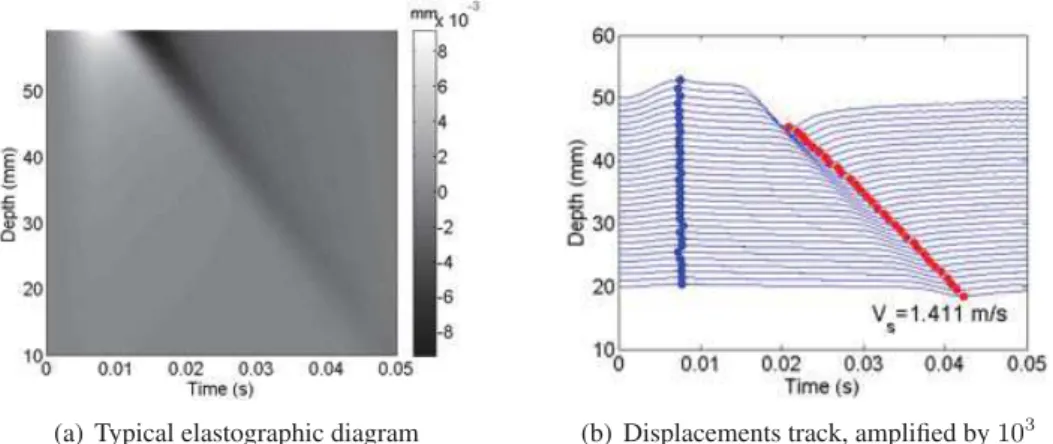
with the package ABAQUS/explicit using standard elements. Fig.1 shows that these elements suffer locking problems and produce an erroneous solution (Fig.1(a)) while the fractional time-step method, both for explicit and semi-explicit schemes, correctly describes the wave propagation (Fig.1(b),1(c)). Besides, the semi-explicit scheme allows for using a much larger time-step than the two others. Fig.2 displays the vertical displacement of a set of nodes located at the left edge of the plate, i.e. right under the prescribed displacement. Fig.2(a) is a typical display of elastographic measurements, Fig.2(b) presents the same data more clearly, each line representing the vertical displacement of one node of this set. The blue peaks illustrate the almost instantaneous P wave propagation while the red valley represents the slower S wave. The latter is the most important in elastography, as its speed is related to the tissue stiffness. After a linear regression, we findVs = 1.411 m/s which is consistent
with the defined material parameters.
The results obtained with the semi-explicit scheme are equally good. Using a much bigger time-step (20 times larger) generates oscillations but after filtering high frequencies, the estimation of the S wave velocity isVs= 1.416 m/s.
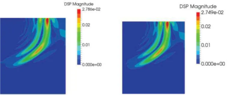
3.2 Heterogeneous test
Here we present a bi-layered model to illustrate the potentiality of the method for characterizing heterogeneous media such as organs with tumors. All the parameters are kept equal to those of the homogeneous case, except for the shear stiffness of the lower part which is increased by a factor5 (C10 = 0.005 M P a). So the S wave speed in the lower part is theoretically 3.16 m/s. In this case,
we used the explicit time integration scheme.
(a) Typical elastographic diagram (b) Displacements track, amplified by 103 Figure 2: Vertical displacements computed by mixed factional time-step elements in explicit
(a) Elastographic diagram (b) Displacements track, amplified by 103 Figure 3: Displacement field for the bi-layered model.
4 CONCLUSIONS
We have presented the adaptability of the fractional time-step method for the simulation of elasto-graphic problems. The method can be easily extended to 3D problems with tetrahedral elements and will help understanding and post-processing elastographic measurements.
REFERENCES
[1] S. Catheline, F. Wu, and M. Fink. A solution to diffraction biases in sonoelasticity: the acoustic impulse technique. The Journal of the Acoustical Society of America, 105:2941–2950, 1999. [2] O.C. Zienkiewicz, J. Rojek, R.L. Taylor, and M. Pastor. Triangles and tetrahedra in explicit
dynamic codes for solids, International Journal for Numerical Methods in Engineering, 43:565– 583, 1998.
[3] S.K. Lahiri, J. Bonet, J. Peraire, and L. Casals. A variationally consistent fractional time-step integration method for incompressible and nearly incompressible Lagrangian dynamics, Inter-national Journal for Numerical Methods in Engineering, 63:1371–1395, 2005.
[4] J. Bonet, H. Marriott, and O. Hassan. Stability and comparison of different linear tetrahedral formulations for nearly incompressible explicit dynamic applications, International Journal for Numerical Methods in Engineering, 50:119–133, 2001.
[5] S. Audi`ere. Signal processing and simulations for ultrasonic elastography , PhD thesis, T´el´ecom ParisTech, 2011.