Creating a Web Page Recommendation System
For Haystack
by
Jonathan C. Derryberry
Submitted to the Department of Electrical Engineering and Computer
Science
in partial fulfillment of the requirements for the degrees of
Bachelor of Science in Computer Science and Engineering
and
Master of Engineering in Electrical Engineering and Computer Science
at the
MASSACHUSETTS INSTITUTE OF TECHNOLOGY
September 2003
@
Jonathan C. Derryberry, MMIII. All rights reserved.
The author hereby grants to MIT permission to reproduce and
distribute publicly paper and electronic copies of this thesis document
in whole or in part.
A uthor ... ...
D
Crtment of ElectriAl Ei'gineering and Computer Science
September 17, 2003
Certified by.
David Karger
Associate Professor
s Supervisor
X
...
Accepted by ..
Arthur C. Smith
Chairman, Department Committee on Graduate Students
MASSACHUSETTS INSTITUTE OF TECHNOLOGY
JUL 2
2
2004
Creating a Web Page Recommendation System For Haystack
by
Jonathan C. Derryberry
Submitted to the Department of Electrical Engineering and Computer Science on September 17, 2003, in partial fulfillment of the
requirements for the degrees of
Bachelor of Science in Computer Science and Engineering and
Master of Engineering in Electrical Engineering and Computer Science
Abstract
The driving goal of this thesis was to create a web page recommendation system for Haystack, capable of tracking a user's browsing behavior and suggesting new, interesting web pages to read based on the past behavior. However, during the course of this thesis, 3 salient subgoals were met. First, Haystack's learning framework was unified so that, for example, different types of binary classifiers could be used with black box access under a single interface, regardless of whether they were text learning algorithms or image classifiers. Second, a tree learning module, capable of using hierarchical descriptions of objects and their labels to classify new objects, was designed and implemented. Third, Haystack's learning framework and existing user history faculties were leveraged to create a web page recommendation system that uses the history of a user's visits to web pages to produce recommendations of unvisited links from user-specified web pages. Testing of the recommendation system suggests that using tree learners with both the URL and tabular location of a web page's link as taxonomic descriptions yields a recommender that significantly outperforms traditional, text-based systems.
Thesis Supervisor: David Karger Title: Associate Professor
Acknowledgments
First, I would like to thank my supervisor Professor David Karger for suggesting this topic and for providing me guidance along the way. Also, Kai Shih helped me during this thesis by discussing his work with tree learning algorithms and providing me with test data from a user study he administered. Additionally, the Haystack research group was invaluable in helping me familiarize myself with the Haystack system. David Huynh and Vineet Sinha were of particular aid in teaching me how to accomplish various coding tasks in the Haystack system and in helping me debug the Haystack-dependent code that I wrote. Finally, thanks to Kaitlin Kalna for being patient and providing welcome diversions from my thesis.
Contents
1 Introduction 15
1.1 H aystack . . . . 15
1.2 Web Page Recommendation . . . . 16
2 Related Work 19 2.1 The Daily You . . . . 19
2.2 News Dude . . . . 20 2.3 MONTAGE . . . . 20 2.4 NewsWeeder . . . . 21 3 Background 23 3.1 N otation . . . . 23 3.2 Probability . . . . 24
3.3 Model for User Interaction . . . . 25
3.3.1 Labeling Links . . . . 25
3.3.2 Hierarchical Correlation . . . . 27
3.4 The Original Bayesian Tree Algorithm . . . . 28
4 The User Experience 31 4.1 Configuring the Agent . . . . 31
4.2 Using the Agent . . . . 31
5 An Analysis of Tree Learning Algorithms 37 5.1 A Weakness in the Original Algorithm . . . . 37
5.2 Fixing the Weakness Using Buckets . . . .
5.3 Developing a Tree Learner Intuitively . . . .
5.3.1 First Attempt at a New Tree Learning Algorithm
5.3.2 Improving the Learner . . . .
5.3.3 Improving the Algorithm Again . . . . 5.3.4 Assessing the Algorithm . . . . 5.4 Weaknesses of the Tree Learning Algorithms . . . .
6 Design of the Tree Learning Package
6.1 Describing a Location in a Hierarchy . . . .
6.2 The IEvidence Interface . . . .
6.3 The ITreeLearner Interface . . . . 6.4 The ITreeLearningParameters Interface . . . .
7 Implementation of the Tree Learning Package
7.1 BigSciNum Prevents Magnitude Underflow . . . .
7.2 Implementing ITreeLearningParameters . . . . 7.3 Implementing the IEvidence Interface . . . . 7.4 Implementing the ITreeLearner Interface . . . . 7.4.1 Implementing a Bayesian Tree Learner . . . . 7.4.2 Implementing a Continuous Tree Learner . . . . . 7.4.3 Implementing a Beta System Tree Learner . . . .
8 The 8.1 8.2 8.3 8.4 8.5 8.6
Haystack Learning Architecture The FeatureList Class . . . .
The IFeatureExtractor Interface .
The ITrainable Interface . . . . Creating General Classifier Interfaces Incorporating Text Learning . . . . . Incorporating Tree Learning . . . . .
40 41 41 43 44 46 47 49 . . . . 49 . . . . 50 . . . . 51 . . . . 52 55 . . . . 55 . . . . 57 . . . . 59 . . . . 61 . . . . 61 . . . . 65 . . . . 68 69 . . . . 70 . . . . 7 1 . . . . 7 1 . . . . 73 . . . . 73 . . . . 74
9 Creating a Web Page Recommendation System For Haystack 9.1 Extracting TreePaths from Resources . . . .
9.1.1 Implementing ResourceTreePathExtractor . . . .
9.1.2 Implementing LayoutTreePathExtractor . . . . 9.2 Getting a List of Links to Rank . . . .
9.3 Ranking Links that Are Found . . . . 9.4 Listening to Changes in Haystack's Database . . . .
9.5 Putting RecommenderService Together . . . .
10 Testing the Recommender System
10.1 Experimental Setup . . . .
10.2 R esults . . . . 10.2.1 Using the URL as the Feature . . . . 10.2.2 Using the Layout as the Feature . . . .
10.2.3 Using the Both the URL and Layout as Features
10.2.4 Using the Text, URL, and Layout as Features .
10.2.5 Composite Versus URL-Only and Layout-Only . 10.2.6 Justification for Negative Samples . . . . 10.3 Summary of the Results . . . .
10.4 Criticism of the Experimental Setup . . . .
11 Conclusion
11.1 Future Work . . . . 11.1.1 Tree Learning . . . .
11.1.2 The Haystack Learning Framework
11.1.3 Recommender Agent . . . . 11.2 Contributions . . . . 101 . . . . 101 . . . . 101 . . . . 102 . . . . 103 . . . . 103 77 77 78 80 81 83 85 86 89 . . . . 89 . . . . 90 . . . . 92 . . . . 93 . . . . 93 . . . . 94 . . . . 95 . . . . 96 . . . . 97 . . . . 99
List of Figures
4-1 The agent setting interface, where the collection of pages to track can
be accessed. ... ... 32
4-2 Web pages can be dragged and dropped into the collection of pages to track.. ... ... ... 33
4-3 The collection of recommended links, after visiting several pages on CNN... ... 34
4-4 An example of active feedback. Note that the page has been placed into the "Uninteresting" category. . . . . 35
6-1 The IEvidence interface. . . . . 51
6-2 The ITreeLearner interface. . . . . 51
6-3 The ITreeLearningParameters interface. . . . . 52
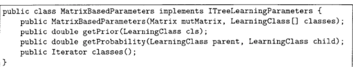
7-1 The public methods and constructors of MatrixBasedParameters. . . 58
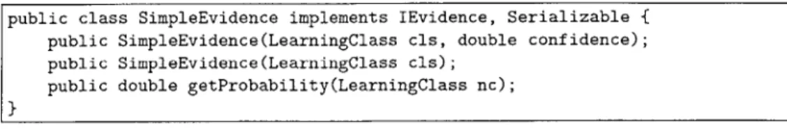
7-2 The public methods and constructors of SimpleEvidence. . . . . 60
7-3 The public methods and constructors of VisitEvidence. . . . . 61
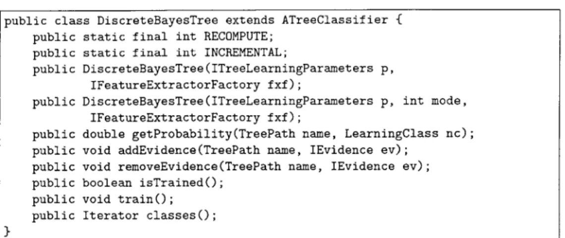
7-4 The public methods and fields of the DiscreteBayesTree class. . . . 62
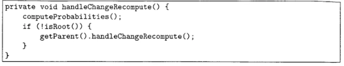
7-5 The private method called to update probabilities when in RECOMPUTE m ode. . . . . 63
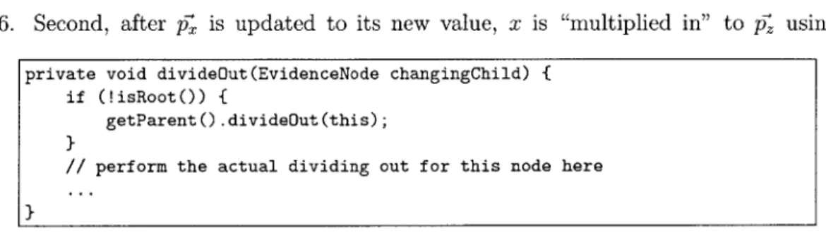
7-6 The private method called to divide out a node. . . . . 64
7-7 The private method called to multiply in a node. . . . . 64
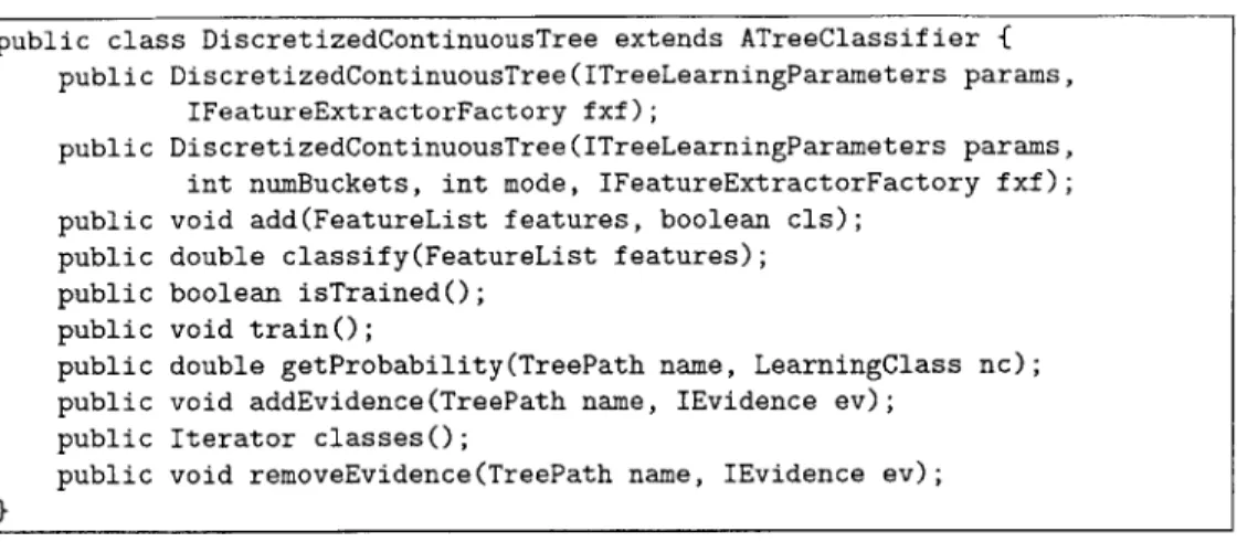
7-8 The class signature for DiscretizedContinuousTree. . . . . 66
8-1 The FeatureList class. . . . . 70
8-2 The IFeatureExtractor interface. . . . . 71
8-3 The ITrainable interface. . . . . 71
8-4 The IBinaryClassifier interface. . . . . 73
8-5 The ATreeClassifier class. . . . . 75
9-1 The ResourceTreePathExtractor class. . . . . 78
9-2 The LayoutTreePathExtractor class. . . . . 81
9-3 The ISpider interface. . . . . 82
9-4 The SimpleSpider class definition. . . . . 82
9-5 The GreedySpider class definition. . . . . 83
9-6 The IAppraiser interface. . . . . 83
9-7 The class definition of URLEvidenceReporter. . . . . 85
10-1 Precision-recall curves for Discrete-U, Beta-U, Buckets-U, Naive-T1, and N aive-T 2. . . . . 93
10-2 Precision-recall curves for Discrete-L, Beta-L, Buckets-L, Naive-TI, and N aive-T 2. . . . . 94
10-3 Precision-recall curves for Discrete-UL, Beta-UL, Buckets-UL, Naive-T1, and Naive-T2. . . . . 95
10-4 Precision-recall curves for Discrete-UL, UL, Discrete-TUL, Beta-TUL, Naive-T1, and Naive-T2. . . . . 96
10-5 Precision-recall curves for Discrete-UL, Beta-UL, Discrete-U, Beta-U, Discrete-L, and Beta-L. . . . . 97
10-6 Precision-recall curves for Discrete-U and Beta-U compared against curves for the same algorithms with no negative samples added. . . . 98
10-7 Precision-recall curves for the Discrete-L and Beta-L algorithms
List of Tables
10.1 Short hand notation for various appraisers, which are described by the
Chapter 1
Introduction
This chapter introduces the context of this thesis, providing basic information about the Haystack information management project and the subfield of web page recom-mendation, which is the driving application of this thesis.
1.1
Haystack
The Haystack project was started because of the increasing need to help users interact with their ever growing corpora of data objects, such as e-mails, papers, calendars, and media files. As opposed to traditional user interfaces, in which distinct applications are used to interact with different types of files using different user interfaces that are each constrained in the way the users view and manipulate their data, Haystack attempts to unify all interaction into a single application. Haystack allows users to organize their data according to its semantic content, rather than its superficial file type.
This unification is achieved by creating a semantic user interface whereby each data object can be annotated with arbitrary metadata in subject-predicate-object format. For example, the paper "Factoring in Polynomial Time" could be listed as having author Ben Bitdiddle, being a member of a set of papers to be presented in at a seminar in the near future, or being in a list of the user's favorite files. The semantic user interface's job is to render data objects given the context in which the user is
browsing to them, and provide appropriate options in the menus for the objects. In addition to providing a uniform, semantic user interface, Haystack provides an architecture for incorporating agents, which are autonomous programs that perform diverse activities such as gathering weather data, automatically classifying data ob-jects into categories, and extracting text from documents. The agent architecture is an excellent setting for creating modules with a large amount of utility for the system. It allows the system to incorporate arbitrarily rich functionality by simply plugging in new agents.
1.2
Web Page Recommendation
In keeping with the underlying goal of helping the user manage large amounts of data, the goal of this thesis is to create an agent for Haystack that searches for new web pages that the user will likely find interesting. In doing so, the agent will decrease the effort a user has to expend navigating to interesting web documents, as well as help the user find both a greater quantity and/or quality of pages.
The recommendation of web pages is an area of active research. Most work in web page recommendation has used textual analysis (See Chapter 2). However, recently, Kai Shih and David Karger have proposed a new feature for learning about web pages [7]. They claim that the URL of web pages bears correlation to many interesting features of a page, such as whether the page is an advertisement and whether the user is interested in the page. They argue that the nature of this correlation is hierarchical; pages with similar URLs, such as the following two
o www. cnn. com/2003/LAW/06/29/scotus .future
o www.cnn.com/2003/LAW/06/29/scotus.review,
are likely to be equally interesting or uninteresting to the user.
Of course, correlation is not necessarily related to the URL's hierarchical
descrip-tion of the page. For example, consider the following two articles:
* www.cnn.com/2003/HEALTH/conditions/07/05/sars.
Both are articles about the SARS disease outbreak and may both be interesting to the user for that reason. Therefore, learning may be able to be improved by incorporating traditional textual methods.
In addition to the URL, the location of a link on a web page (e.g. first table, fourth element, second subtable, fifth element) is likely to be correlated to a user's interest in the link's contents. To make web pages more useful to visitors, web editors have an incentive to localize links to web pages that users will be interested in, because a user is unlikely to scrutinize an entire web page to examine all of its links. For example, visitors to CNN's home page may be too busy to look at all of its approximately 100 links; they may only look at headline news stories or at links that appear under their favorite subheading.
This thesis seeks to implement the web page recommending capability of Shih's "The Daily You" application by exploring the benefits of traditional textual analysis, as well as implementing the idea of learning over a hierarchy using the URL and tabular location of links. In addition, it seeks to provide robust interfaces for the recommendation of web pages that will allow new algorithms to be plugged into the recommender agent without requiring the whole agent to be rebuilt from scratch.
Chapter 2
Related Work
This chapter describes Kai Shih's The Daily You application, which was the motiva-tion for this thesis, as well as a few other web page recommending systems that have been built.
2.1
The Daily You
The Daily You is an application that Kai Shih developed to recommend new inter-esting web pages [7]. The user gives the application a list of web pages to track, and uses the history of a user's clicks to provide a set of positive samples, which serves as the training data. Then, using both the URL and the tabular position of links, it recommends the top stories from each page it is tracking.
In addition, The Daily You cleans the pages that are displayed by blocking ads and static portions of web pages, such as the table of links to the various sections of a news website.
The algorithm that The Daily You uses to learn trends in URLs and tabular locations of links is a tree learning algorithm that uses a tree-shaped Bayesian network
(See Chapter 3 for more details).
The high level functionality of the agent created in this thesis essentially emulates the web page recommending functionality of The Daily You, using a generalized version of Shih's algorithm as well as other tree learning algorithms developed in this
thesis, although it is not necessary for the agent created in this thesis to exclusively use tree learning algorithms.
2.2
News Dude
Billsus and Pazzani's News Dude recommends news stories [2], with some emphasis placed on the development of a speech interface. To learn which stories are interesting, it uses the well-known Naive Bayes and nearest neighbor algorithms on the text of the stories.
It is similar to the agent built in this thesis in that it customizes recommendations to the individual user. However, it is different in that it only uses textual analysis of the news stories and in that it requires active feedback. By contrast, the recommender agent in this thesis learns user preferences by using any binary classifier, including tree learners that do not even use text. Also, it uses passive feedback, while allowing active feedback via Haystack's categorization scheme, so that users are not required to exert any effort for the agent to learn.
One other interesting aspect of News Dude is that it attempts to differentiate short-term user interests from long-term interests, so that it captures fleeting trends in users' tastes. The agent built in this thesis does not attempt to make such a distinction.
2.3
MONTAGE
Corin Anderson and Eric Horvitz developed the MONTAGE system, which tracks users' routine browsing patterns and assembles a start page that contains links and content from other pages that the system predicts its users are likely to visit [1].
One of their important ideas for the learning process of MONTAGE was to note that the content that users find interesting varies depending on the context of the web access. In particular, their application uses not only the URLs of websites that are visited but also the time of day during which the access occurs. As a result,
recommendations may change as the time of day changes.
Another interesting aspect of MONTAGE is that when agglomerating the start page, it considers not only the probability of a user's visiting the page in the current context, but also the navigation effort required to reach the page. Thus, between two pages that are equally likely to be visited, MONTAGE fetches the one that would require more browsing effort to reach.
Compared with the agent built in this thesis, MONTAGE is similar in that it uses features of web pages other than the text when recommending content to users. However, the underlying goal of the recommender agent is not exactly the same as
MONTAGE. While MONTAGE strives to assist users in routing browsing to various
web pages that are frequently visited, the recommender agent searches for links to new stories that have not yet been visited.
2.4
NewsWeeder
Ken Lang's NewsWeeder project is a netnews-filtering system that recommends doc-uments leveraging both content-based and collaborative filtering, although the em-phasis is on content [5]. NewsWeeder asks users for active feedback, which it uses in conjunction with textual analysis to improve future recommendations to its users. Lang introduces a Minimum Description Length heuristic for classifying new doc-uments by their text, which he reports compares favorably to traditional textual analysis techniques.
NewsWeeder differs from the agent in this thesis in that it requires active feed-back rather than simply allowing it, and in that uses only textual analysis to learn preferences.
Chapter 3
Background
This chapter introduces notation, terminology, and concepts that are essential to learn in order to fully understand the rest of this thesis.
3.1
Notation
Some custom notation is adopted to simplify probabilistic analysis of the tree learning algorithms in this thesis. This section introduces the notation for representing prob-abilities and other values associated with a tree learner, such as the discrete Bayesian tree learner described in Section 3.4.
Trees will be described as if their roots are at the top, so that children are further down in the tree and a node's parent is higher up. The variables i, j, and k will usually be used to represent classes to which a node may belong, while the variables
X, y, and z will usually represent specific nodes in the tree. Expressions of the form xi will be used to represent the event that the specified node (in this case x) is of the specified class (in this case
j).
The value p' will be used to represent the probability of all of the evidence in the subtree rooted at node x, conditioned on the hypothesisz1, that x is of class i. The value Pk will be used to represent the prior probability
3.2
Probability
This section provides an overview of some of the basic probability concepts that are necessary to understand the algorithms in this thesis. David Heckerman has written an excellent tutorial on learning with Bayesian networks, of which the original tree learning algorithm is a specific example [4]. This tutorial was consulted for ideas about how to improve tree learning.
First, it is essential to understand Bayes Rule in the following form
Pr[AIB] Pr[B] = Pr[A A B] = Pr[BIA] Pr[A]. (3.1)
In particular, this rule implies that the probability of event A occurring given that B has occurred can be computed by the probability of both A and B occurring divided
by the probability of B occurring. This implication is used by the original discrete
Bayesian algorithm introduced in Section 3.4.
Second, it is important to have a general understanding of the Beta distribution, which is used, for example, in the discretized continuous Bayesian tree learner im-plemented in this thesis. In that tree learner, the Beta distribution is used as the probability distribution of each node's children (See Section 5.2). Although there is a lot that can be said about the derivation of the Beta distribution, its expectation, and how to set its prior, understanding these is not essential to understanding how it is used in this thesis. Therefore, only the basic characteristics of the Beta distribution are discussed here.
Basically, the Beta distribution is a distribution that is only positive for values in the interval [0,1]. The shape of a Beta distribution is a quasi bell curve, centered around its expectation, which can be computed from the number of positive samples
ni and negative samples no upon which the distribution is based. The expected
fraction of Beta distribution samples belonging to the positive class has the simple closed form
(3.2)
A Beta distribution has 2 important parameters for establishing a prior
distribu-tion:
" ao, which represents the number of "virtual negative samples"
" a1, which represents the number of "virtual positive samples"
The expected fraction of Beta distribution samples belonging to the positive class has the simple closed form
ni + eei (3.3)
ni + no + a1 + ao when a prior is used.
The Beta distribution is commonly used in applications because it has positive values exactly on the [0, 1] interval, its expectation has a simple formula, and because its prior can be set intuitively by adding "virtual samples."
3.3
Model for User Interaction
In this section, a model for user interaction is presented that motivates the devel-opment of tree learning and provides a concrete model against which to judge the aspects of various tree learning algorithms.
3.3.1
Labeling Links
Suppose a user browses a front page, such as CNN's home page every day. During that time, the user will click on some subset of the links that appear on the page that day. The goal of web page recommendation is to determine which links the user will click during the next day, when many new links are available. Although the user has not provided any feedback regarding new links, there may be feedback for many similar old links, such as links from the same part of the page or having similar URLs. To compute the probability that a new page is interesting, it would be intuitive to use the fraction of similar old links that were visited. For example, if there are 12
similar URLs and 3 were clicked, then it is reasonable to believe that there is about a 25% probability that the new link will be clicked.
One question that remains is how positive and negative examples should be added. One strategy is simply labeling nodes as clicked versus not clicked. In such a strategy, unvisited links would be used as negative samples until the user visits them, if ever, while repeated visits to the same page would be ignored. This strategy is simple and intuitive, but there are other aspects of web pages that merit discussion.
The simple setup ignores the fact that some nodes have more "facetime" than oth-ers. For example, a link to a section heading, such as http: //www. cnn. com/WORLD/, may persist indefinitely, and if the user ever clicks on this link then it will be labeled as good, even if the one time that the user visited the link was by accident.
To provide a simple example of how this can cause problems, assume that a user clicks on all of these section headings at least once, even though none of them is particularly interesting. If a new section heading appears, it will be heavily supported because 100% of the similar links were clicked. On the other hand, if a user reads
60% of all of the health articles that are posted, then the user is likely more interested
in a new health article than in a new section heading.
This issue motivates the practice of adding multiple pieces of evidence to the same link, one for each time the page is sampled. For example, suppose the page is sampled once day, and every link that has been clicked during the day has a positive label added to it and every page that has not been clicked has a negative label added to it. Then, 60% of the health labels will be positive, while many negative samples mount for the static, section links, so that perhaps only 5% of them may be positive.
The implementation of passive evidence gathering in this thesis is that each time the agent runs, all visited links are gathered as positive samples for the classifiers, and an equal number of negative samples are randomly picked off of the pages being tracked, from the subset of links that were not visited since the last time the agent ran. This choice retains all positive samples while keeping the total number of samples manageable because the number of samples is proportional to the number of times a human clicked on links.
As an aside, if the goal is to recommend pages that the user wants to read, then using clicks as a proxy is not a perfect solution because a user's clicks do not neces-sarily directly lead to interesting web pages. For instance, the user may mistakenly open a page, or use a link as an intermediate point while navigating to an interesting page. However, to avoid requiring active feedback, it was deemed the best proxy to use for passive feedback.
3.3.2
Hierarchical Correlation
New nodes are likely to have many nearby nodes in the tree with many pieces of evi-dence. However, when new nodes appear that do not have many immediate neighbors, the hierarchical correlation assumption can be used to to provide prior knowledge about the likelihood that the new node is in each class. The hierarchical correlation assumption states that children and parents are likely to be of the same class.
The reason why the assumption about hierarchical correlation is expected to hold when the tabular location of a link is used as a feature is that web editors have an incentive to localize stories of similar degrees of interest to users. By clustering links as such, they decrease users' costs of searching for what they want to read, making the user more likely to return to the website in the future. Because nearby links are close together in the tabular layout hierarchy of a web page, it is reasonable to assume that the hierarchical correlation assumption holds.
The reason why the correlation assumption is expected to hold for the URL feature is similar. The subject matter of an article is often correlated to its URL as evidenced
by various news sites, such as CNN, that organize their stories into sections, which
appear in the URLs for the stories. Also, the URL can convey even more information than merely the subject. For instance, if a page has a section with humorous articles, the humorous articles may have similar URLs, but assorted subject matter.
3.4
The Original Bayesian Tree Algorithm
This section describes the original tree learning algorithm that was developed by Shih [7]. Essentially, Shih's algorithm solves the problem of binary classification by computing, for each node x in the tree, the probability p' and px, the probability of the evidence in the subtree rooted at x given that x is of type 1 (has the trait) and of type 0 (lacks the trait). Let p1 and p0 represent the prior probabilities that the root is of types 1 and 0 respectively. The probability that a new node n has that trait can be computed using Bayes' Rule as the probability of the evidence underneath the root,
P Poot +P 0 0?t, given that the new node has the trait, divided by the probability of the evidence in the tree
Pr[n1 /\ all evidence]
Pr[nl Jall evidence] Pr[ all evidence] (3.4) Pr[all evidence]
Shih's algorithm computes each px and po by modeling the tree as a Bayesian network, so that
PX = Mnlp,
+
Mo1p0yEchildren(x)
px = Moop" + M104p,
yEchildren(x)
where Mij is the probability that the child's class is i given that the parent's class is
j
(Mij can be thought of as probability of a mutation between generations in the tree that causes the child to be of class i when its parent is of class j). The leaf nodes,z, are the base case of this recursive definition; for example, pl is set to 1 if the leaf represents a positive sample and 0 if the leaf represents a negative sample.
In this thesis, this algorithm was generalized to handle an arbitrary number of classes (other than just 1 versus 0) by redefining the probabilities at each node to be
-
H
Z
s ,(3.5)for each class i.
One asset of this algorithm is that it yields an efficient, incremental update rule. When a new leaf x is incorporated into the tree, one way to update the pi values for each node z in the tree is to recompute all of the values recursively as Equation 3.5 suggests. However, a key insight that leads to the fast incremental update algorithm is that most of the values of p' in the tree remain the same after a new piece of evidence is added because none of their factors have changed, which follows from the fact that no evidence in their subtrees have changed. The only p's that have changed lie on the path from the newly added leaf up to the root.
Each changed p' will need to have exactly one factor changed, the factor corre-sponding the the child that has changed. These changes are made from the bottom up; the parent y of the leaf has each of its p, s modified to incorporate the new factor from the leaf, then the grandparent divides out the old values of p and multiplies in the new ones. Removing leaves can be accomplished analogously. For further details regarding how the incremental update rule is implemented, including pseudocode, see Section 7.4.1, which describes the implementation of the discrete Bayesian tree learner implemented for this thesis.
Chapter 4
The User Experience
This chapter describes the experience that a user has while configuring and using the recommender agent that was developed in this thesis.
4.1
Configuring the Agent
When running Haystack, a user can open up the settings to the recommender agent
by searching for "recommender agent." At this point, the user will be presented with
the interface shown in Figure 4-1.
The one pertinent setting is the collection of pages to track. In order for users to be recommended web pages, they must provide the agent with a starting point or points to begin searches for links to new pages. The collection "Pages to Track" is just like any other collection in Haystack, web pages can be added to it via Haystack's drag and drop interface. As an example, Figure 4-2 shows a screenshot of the collection of pages to track after CNN's homepage has been dragged into it.
4.2
Using the Agent
Once the collection of pages to track has been formed, the recommender agent will be-gin recommending links that appear on those pages. The collection of recommended links is maintained by the recommender agent and updated periodically
through-IS Haystack Home Page
U?] Fiesystem
V& Set up messaging and news
Figure 4-1: The agent accessed.
Settings
Coilection of pages Q Pages to Track to track
Agent/Service Summary
rtlecommender Agent
Description Ths agent recommends web documents. Add
Works for L Jonathan Derryberry nearby
AN PrQpertbi Standard Propertim
setting interface, where the collection of pages to track can be
out the day. To view the recommendations, the user can search for the collection "Recommended Links," and keep the collection on one of the side bars, as shown in Figure 4-3.
Although the recommender agent will be able to make recommendations based on passive feedback obtained by listening to all of a user's visits to web pages, users also have the option of providing active feedback by categorizing web pages that they view. This functionality is shown in Figure 4-4.
ULated ;44 pm MT -Q24 OUT) Auut, Z203
Figure 4-2: Web pages can be dragged and dropped into the collection of pages to track.
Figure 4-4: An example of active feedback. the "Uninteresting" category.
Chapter 5
An Analysis of Tree Learning
Algorithms
Before delving into the design and implementation of the recommender agent, the new tree learning algorithms that were developed for this thesis will be discussed in this chapter.
In the beginning of this chapter, a potential fault in the original discrete Bayesian algorithm (See Section 3.4) is identified and explained. Consequently, two alternative algorithms, one of which is a variant of the original, are proposed to rectify this weakness.
5.1
A Weakness in the Original Algorithm
The Bayesian tree learning algorithm has many good traits. It has a fast, incremental update procedure, and it seems to provide good performance in the setting in which only positive examples are used. However, there are some troubling aspects that could cause the algorithm to produce undesirable results.
First of all, if the user interaction model presented in Section 3.3 is accepted, then providing negative examples is important to producing good results. The intuition behind this claim is that without negative samples, a tree learner is likely to recom-mend the types of links that are visited most frequently as opposed to the types of
links that are visited with the highest probability, such as rarely appearing links that are always visited on the rare occasions that they appear (e.g. a breaking news alert).
Second, if negative examples are used in the discrete Bayesian algorithm described in Section 3.4, then the ranking of the quality of a node in relation to others depends systematically on the number of nearby samples. To illuminate this problem, a toy example will be analyzed and then intuition for the problem will be presented.
Consider the example of a root node, r, that has C children, a fraction a of which are good (class 1) as supported by all of the data that has been gathered so far. If an unknown node x appears that is a child of r, we can compute the probability that it is good by using Equation 3.4 as follows
Pr[all evidence A xl] Pr[ all evidence] =ei
Pr[all evidence](51
Where x1 represents the event that new node x is of type 1. The probability of the evidence is given by the following formula
Pr[all evidence] = p1pl + p P,0
= P
J7
(Mp + Moip0)+p 01
(MoopO + Miop )yEchildren(r) yEchildren(r)
Plugging the in the terms for the children, this becomes
Pr[all evidence] = pl(MaCM C( "a) + (MQOCM C(l0a)). (5.2)
Now, under the reasonable and simplifying assumption that pl = p0 = and that
M = M10, this reduces to
Pr[all evidence] = 1 [(1 - /3)acfc(1-a)] + 1 [ac (1 - )C(1-a)] , (5.3)
2 2
extra factor into each of the terms, resulting in
Pr[all evidence A
xl]
=[(1
- 3)OC+113C(1-c)]+
[ac+1(1 - O/C(1-a)] , (5.4)which makes Pr[x' I all evidence] reduce to
Pr[xl | all evidence] 1( - 3)ac+1OC(1-o)] +
[
aC+1(I- O)C(1-a) = [(1 _ 3)QC3C(1-O)]+ 1 [/3C(i _ 3)C(1-a)]
(1 - 3)QC+13C(1-a) + Oac+1(i - O)C(1-a)
(1 - #)acoc(1.-a) + Oac(I - 3)C(1-a)
(1 - O)OC(1-2a) + 0(1 - O)C(1
-2a)
-3C(1-2c) + (1 - O)C(1-2a)
Now, we are ready to examine the effect of a and C on the recommedations that would be made by the algorithm. First of all, note that the only place a and C come into effect is in the exponents, by the value C(1 - 2a) = C(1 - a) - Ca, which is
simply the difference between the number of positive samples and negative samples, not their ratio. An example will illustrate this: let C = 100 and a = 0.3, yielding
Pr[x(
I
all data]
1 - 0)100(0.4)] + [0(1 _ 0)100(0.4)] [/3100(0.4)] + [(1 - 0)100(0.4))][(1
- 3)040] + [/3(1 - )40][/340] + [(1 - 0)40]
Compare this to the case in which C = 200 and a = 0.4
Pr[xl all data] [ ( - 0)200(0.2)] + [/(1 - 0)200(0.2)] [/200(0.2)] + [(1 - 0)200(0.2))
[(1 - 0)040] + [/(1 - 0)40]
[40] + [(1 - /3)40] .
In this example, the second case had a higher fraction of positive examples, but was declared equally likely to be good because it had more samples. With a little further inspection, it is clear that if the second case had more samples, it would be predicted as being less likely to contain a new positive node than the first case. In fact, in both
cases, assuming that (1 - 13)4 dominates the f 40 term, the predicted probability that a new node is good is about 13, the mutation probability, which could be far less than either 0.3 or 0.4. If 3 = 0.1, then the predicted probability that the new node is good
would be about 0.1, which runs contrary to the intuition that it should be predicted to be good with probability 0.3 or 0.4.
Although this is only a toy example with a parent and one generation of children, it is clear that the underlying cause of the problem extends to the algorithm when applied to a whole tree. In fact, some thinking about the assumptions the algorithm makes about the underlying model sheds light on the root of the problem in this application: the binary probability space is incapable of capturing a phenomenon that is inherently continuous. In other words, the discrete Bayes algorithm tries to determine whether each node is "good" (i.e. has 90% good children) or "bad" (i.e. has
10% good children). There is no notion of "excellent," "very good," "average," and
so on. However, to create an ordered list of recommendations that places excellent leaves ahead of very good leaves, it is necessary that the tree learner be able to make such a distinction because being very confident that a node is good is different from predicting that the node is excellent.
In order for the binary discrete tree learner to avoid this problem, the underlying process it is modeling must exhibit data that corresponds to its model, for example if the children of nodes in a tree were found to either be roughly 90% good or roughly
10% good, then the binary discrete tree learner would model the process well if the
mutation probability were set at 10%. However, this appeared empirically not to be the case with web page recommendation.
5.2
Fixing the Weakness Using Buckets
Once this problem is identified with the discrete Bayes tree, one potential solution is to simply make the parameter space continuous, to reflect the true underlying process (e.g. clicks correlated to URLs or page layout). However, the problem with this is that it is a daunting task to model a continuous parameter space in a Bayesian net
efficiently, as there are an infinite number of "classes" about which to store proba-bilities. However, making the complete transition to a continuous parameter space is unnecessary for most applications. One alternative is to discretize the parame-ter space into a finite number of buckets, which could represent, for instance, 0.5% good, 1.0% good, 1.5% good, et cetera, assuming that users will not care whether a document is 52% good or 52.5% good.
Using the generalized, multiclass version of the discrete Bayesian tree learning algorithm makes this transition easy; new classes are made to correspond to each bucket. The only thing left is to determine what the conditional probabilities of the children are given the parent nodes. A natural choice is to assume that the children's parameters are distributed according to a Beta distribution, centered about the parent's bucket.
The beta distribution is a good choice because it is assigns a positive weight to exactly the buckets on the interval [0, 1] and is shaped like a bell curve centered about its expectation. Also, a prior can easily be placed on the distribution, if desired, to push the distribution of children slightly toward some a priori determined Beta distribution.
5.3
Developing a Tree Learner Intuitively
In addition to fixing the weakness using buckets, there are other alternatives for making a tree learner that is more amenable to solving problems with a continuous parameter space. This section describes an algorithm that was developed intuitively. Although it was not developed according to any probability model, it runs in linear time with a small constant, and directly addresses the problem with the discrete Bayes algorithm.
5.3.1
First Attempt at a New Tree Learning Algorithm
Let the vector 52 contain a histogram for the set of observations for some node x; for example, 5, = (23,44) if there were 23 positive examples and 44 negative examples
contained in the set of leaves below x. Also, let p-be a vector with values representing prior beliefs about the ratio of the distribution of the evidence, normalized so that its entries sum to 1; for example, p'might equal (0.2, 0.8) if each node in the tree was expected to have 20 percent positive examples. Now, define a constant a to be the weight given to p. This weight can be thought of as the the number of imaginary observations that p represents. Define the predicted distribution of the classes of new leaves below x to be
S= a(5.5),j
where Ox represents the total number of samples for node x. For instance, continuing using the above example values, and if a = 30, then Equation 5.5 becomes
(23,44) + 30(0.2, 0.8)
fX 67 +30
29 68)
This provides a suitable solution if there are many observations, or if there are no known correlated observations from other sets. However, when learning over a hierarchy, it is natural to have nearby nodes, such as children and parents, affect our beliefs about the probability distribution
fx,
especially if there are few observations for x, but many observations for the parent, y, and some children, z, of node x. From our assumptions, data collected from a single node are assumed to come from the same distribution f and the distributions f and f of the parents and children are believed to correlate tofx
although there may be differences, which are expected to be slight, but possibly large.Assuming that the severity of differences in distributions between neighbors is independent of their locations,
fy
andfz
for each child z can be incorporated, with equal weight intof
as follows.
d+ a,+ 0-(x)
O + a n (5.6)
words
fy + Ezechildren(x) f.
1 + |children(x)1 (57)
Although this definition for fx is circular, fx can be found for each node in the tree simultaneously because the equations for all of the fxs can be collected and solved as a system of equations.
5.3.2
Improving the Learner
Although the learner from the previous section seems to satisfy most of our intuition about how to learn over a hierarchy, there is a troubling caveat. Consider the following two scenarios:
" There is a root with little evidence but one child with much positive evidence " There is a root with little evidence but many children, each with much positive
evidence.
Intuitively, the second scenario should cause the root to be more positive than in the first because there are more child nodes supporting the hypothesis that it is positive. However, the above framework does not allow for this because all of the children are lumped together into one sum, which is normalized by the number of neighbors.
An alternative to the above algorithm is to lump the a' term and the neighbors term (On'(x)) together into one term that weights fx toward its distribution. Intu-itively, this model maintains the nice feature that real observations at each node can outweigh the effect of its neighbors and a term, but adds the feature that a higher number of neighbors diminishes the effect of the a priori determined a term. In this setting, the distribution that will weight fx can be expressed as
13P Eyeneighbors(x) fy
Px /+Ineighbors(x)| (5.8)
where 'o can be thought of as the expected value of the distribution at node x (igoring leaves beneath x), - can be thought of as the a priori determined expected value for
the distribution of an arbitrary node in the tree, and 3 is the number of "virtual neighbors" that p represents. Then,
f,
can be defined asox + ay , (5.9)
which can be solved as a system of equations as the previous algorithm can.
5.3.3
Improving the Algorithm Again
One problem with the previous algorithm is that the distribution of a node is changed when children are added to it, even when they contain no evidence. For example, consider a parent node that has a fraction 0.7 of positive samples but, because of the weighting term, reaches an equilibrium with a value of 0.6 attached to the positive class. If a new node with no evidence were added as its child, then the parents's predicted fraction of positive samples may increase because the child will inherit its distribution from its parent, and the parent will perceive this as more evidence that its higher fraction of positives is correct. This does not make sense; although a new node has been added, no evidence has been added to the tree.
To be exact, there are two problems that can cause undesirable behavior from adding an empty node
1. The imaginary data from the weighting term affects neighboring nodes, even if
the affecter is an empty leaf node.
2. Data from a single node is allowed to reflect back to itself as it propagates through the tree.
One solution to the first problem is to weight the average of the neighboring nodes so that nodes with little or no evidence have little or no influence on their neighbor's distributions. To present the solution, define the distribution of a node as usual to
be
with - redefined to be
3 yEneighbors(x) W~f Y
pOP (5.11)
13 +..yEnezghbors(x) Y
where W, is a weight term that ensures that neighbors with a small amount of data in their branches do not carry much weight when taking the weighted average of neighboring nodes.
A reasonable definition for W, is the fraction of y's distribution that is based
on real data, either in the node itself or from its neighbors. From Equations 5.10 and 5.11, W, is thus defined as
W 1 -
).
(5.12)Y a Y + EzEn hbssoy) Wz
However, this strategy only solves the problem of imaginary data being regarded as real data if the weights for nodes whose branches contain no data are 0, and because data flows all around the tree, this may not be the case. Nevertheless, also incorporating a solution to the second problem from above will solve the first problem completely.
To prevent data reflection and solve the second problem listed above, a new set of distributions hx,y is defined such that each hx,y is the distribution that y sees coming from its neighbor x. The value of hxy is declared only to be influenced by nodes in y's branch to x (i.e. all nodes that y must reach via a visit to x). Each hx, can then be defined as
Ox
+ a
Z zEneighbors()-y Wz'xz-axzy = -g"b"r- w, , (5.13)
where Wz,x is defined (similarly to WY) as
W( x =n 13
(
. (5.14)Finally, with the distribution of an arbitrary node x again defined as
fX
= ,x (5.15)but with ' redefined to be
_3r + EyEneighbors(x) WYxy,x
p, =-:: (5.16)
both problems from above are solved.
A positive attribute of these definitions is that they yield an algorithm that can be
solved in linear time; each fx can be solved for explicitly and efficiently. Computing Wxy and hxy for all distinct x, y E T requires only O(n) time because Equations 5.13 and 5.14 can be applied directly for each pair of neighbors in the tree if the tree is traversed in postorder first to compute the bottom up values and in preorder second to compute the top down values. Then, all of the knowledge exists to compute each fX
directly from Equations 5.15 and 5.16. Pseudocode for this algorithm is omitted for the sake of simplicity, although implementing the algorithm is straightforward from the equations.
5.3.4
Assessing the Algorithm
Although its genesis is based on intuition about the specific problems of learning about
user interests over the hierarchy of URLs and tabular locations, and the algorithm may not be a good choice for tree learning in other contexts, the proposed tree learning algorithm has many positive attributes:
" No matter how many confident neighbors a node has, a significant number of
observations at a node will outweigh the influence of the neighbors. This is because the aggregate effect of the neighbors is grouped into one term whose weight cannot exceed a constant number of real observations for the node.
distribu-tions of the other nodes in the tree.
" The computed distribution at evidenceless nodes that have many neighbors with
the same distribution is closer to the distribution of the neighbors than if there were only one or two neighbors.
" The algorithm is efficient; it can be trained from scratch in linear time with a
relatively small constant.
5.4
Weaknesses of the Tree Learning Algorithms
All of the tree learning algorithms mentioned in this thesis suffer from weaknesses
resulting from the rigid tree structure that the tree learning framework imposes. All of them assume that the likelihood that a node is good can be completely encapsulated
by the node's immediate neighbors. However, this is probably not true in general for
either URLs or tabular locations.
In URLs, often times a parent will receive negative samples, but nevertheless have children with very positive distributions. For example suppose a user never clicks on any links to
http: //www. cnn. com/WORLD/<region>, but nevertheless often clicks on links of the form
http: //www. cnn. com/WORLD/<region>/<story>. Any of the above algorithms will deduce that a link of the form
http: //www. cnn. com/WORLD/<newregion>/<story>
is bad because it is a direct descendant of a node that received a lot of negative evidence. There is no way to recognize that grandchildren of the WORLD node are usually good to recommend.
Another problem occurs when web editors place meaningless, dynamic information into URLs. For example, CNN places the date in their URLs, although this will probably not be a significant factor in whether or not a user wants to read the story.
This same problem occurs when using the layout of web pages. Home pages sometimes add or remove banners or other elements on their web pages, or move tables around in the page. Often much of the underlying structure of the layout remains the same. For instance, a headline news story may have location [2,3, 0, 0,2] one day, but the next day an extra banner may be put into the page, making the layout position [3, 3, 0, 0, 2].
To some extent, these problems can be solved heuristically, for example by deleting dates from URLs. However, an ideal tree learning algorithm would be able to deal with these problems gracefully without needing heuristics. One potential solution is to use a variant of nearest neighbors, defining the distance between two nodes to be the edit distance between two hierarchical descriptions. However, efficiently implementing such an algorithm would be a challenge and there would still be systematic problems with a straightforward nearest neighbors implementation (e.g. how to choose between equally distant neighbors).
Chapter 6
Design of the Tree Learning
Package
The functionality of the tree learning package was based on the tree learning frame-work developed by Shih [7] (See Section 3.4). To maximize the utility of the tree learning architecture in this thesis, it was designed to be independent of the docu-ment recommender system as a whole. In fact, there is no reason why it cannot be used to learn about hierarchies of documents other than web pages, or even objects other than documents, such as photographs or animals, provided there is a hierarchi-cal description of them.
Thus, the recommender system as a whole is merely one example of how to use the tree learning framework to learn about hierarchical data. At a high level, the tree learning architecture presents an interface in which the user of the learner adds evidence associated with a hierarchical description of an object to a tree learner. The user can also query nodes to determine the probability that the queried node is of a specified class.
6.1
Describing a Location in a Hierarchy
Locations of nodes in hierarchies can be described in diverse ways. Rather than use a string such as "http: //www. cnn. com/BUSINESS," "200 Technology Square,
Cam-bridge, MA U.S.A.," or "first table, third element, second subtable" to describe the location of a node in a tree, the hierarchical name of a node was abstracted using the TreePath class, provided by Java.
The constructor takes an array of objects representing a downward path, from the root toward the leaves, of a node in a hierarchy. The purpose of using the TreePath class as opposed to the URL directly is to make the tree learner flexible about what form the hierarchical description of a node may take; in other words, it provides a layer of abstraction between the hierarchy and how it is described. It is left up to the user of the tree learner to transform the features of their particular taxonomies into TreePath objects for use with the tree learning architecture. For example, users may change names such as "http: //www. cnn. com/BUSINESS" and "200 Technology
Square, Cambridge, MA U.S.A." into "[com, cnn, BUSINESS]" and "[U.S.A., MA,
Cambridge, Technology Square, 200]."
6.2
The IEvidence Interface
Usually in tree learning or classification, the evidence objects added to nodes are merely labels corresponding to which class the nodes belong. However, the tree learning architecture was made more flexible so that the Bayesian algorithms could make use of their full power.
Each p' in a Bayesian tree represents the probability of the evidence in the subtree rooted at x given that x is of type i. Thus, a piece of evidence in a tree need not be a simple label; it can have its own values of p" defined. For example, suppose a fire engine is red with probability 0.9 and a sports car is red with probability 0.3. Then a leaf representing the evidence "is red" would have avesj p fire red "ng"ne= - 0.9 and Pis red car _prs =0.3.
To encapsulate the abstract notion of evidence, the IEvidence interface was writ-ten (See Figure 6-1). Its one method, getProbability, returns the probability that an object would exhibit the evidence if its class were cis (i.e. Pte evidence)' an object
of type LearningClass (a class to abstractly represent the identity of the classes to which a node may belong).
public interface IEvidence {
public double getProbability(LearningClass cls); }
Figure 6-1: The IEvidence interface.
Also, for the specialized purpose of doing tree learning over two classes, the child interface IBooleanEvidence was created.
It should be noted that not all tree learning algorithms can easily make use of this generalized evidence framework. For example, the intuitive algorithm developed in Section 5.3 may produce undesirable results if used with evidence other than labels with variable confidence. For this reason, in hindsight, it may be desirable to change the IEvidence interface so that it only represents labels, with variable confidence.
6.3
The ITreeLearner Interface
The interface for tree learner objects is similar to other machine learning interfaces, containing methods for adding new training data and testing new objects. On the other hand, the tree learning framework is different from other machine learning interfaces because it requires that all objects used in training or testing have a hier-archical description, whether it be a URL or a taxonomic name of an organism. The
ITreeLearner interface appears in Figure 6-2. public interface ITreeLearner {
public double getProbability(TreePath name, LearningClass cls); public void addEvidence(TreePath name, IEvidence ev);
public void removeEvidence(TreePath name, IEvidence ev); public Iterator classeso;
}
Figure 6-2: The ITreeLearner interface.
The addEvidence method associates the evidence ev, an object that implements the IEvidence interface, with the entity described by the TreePath name, which may contain something like the sequence of words "[com, cnn, LAW, petersoncase." The removeEvidence method functions analogously. The getProbability method