HAL Id: hal-01479240
https://hal.inria.fr/hal-01479240
Submitted on 28 Feb 2017
HAL is a multi-disciplinary open access
archive for the deposit and dissemination of
sci-entific research documents, whether they are
pub-lished or not. The documents may come from
teaching and research institutions in France or
abroad, or from public or private research centers.
L’archive ouverte pluridisciplinaire HAL, est
destinée au dépôt et à la diffusion de documents
scientifiques de niveau recherche, publiés ou non,
émanant des établissements d’enseignement et de
recherche français ou étrangers, des laboratoires
publics ou privés.
Learned features versus engineered features for
multimedia indexing
Mateusz Budnik, Efrain-Leonardo Gutierrez-Gomez, Bahjat Safadi, Denis
Pellerin, Georges Quénot
To cite this version:
Mateusz Budnik, Efrain-Leonardo Gutierrez-Gomez, Bahjat Safadi, Denis Pellerin, Georges Quénot.
Learned features versus engineered features for multimedia indexing. Multimedia Tools and
Applica-tions, Springer Verlag, 2016, 76 (9), pp.11941-11958. �10.1007/s11042-016-4240-2�. �hal-01479240�
(will be inserted by the editor)
Learned features versus engineered features for
multimedia indexing
Mateusz Budnik · Efrain-Leonardo Gutierrez-Gomez · Bahjat Safadi · Denis Pellerin · Georges Qu´enot
Received: date / Accepted: date
Abstract In this paper, we compare “traditional” engineered (hand-crafted) features (or descriptors) and learned features for content-based indexing of image or video documents. Learned (or semantic) features are obtained by training classifiers on a source collection containing samples annotated with concepts. These classifiers are applied to the samples of a destination collec-tion and the classificacollec-tion scores for each sample are gathered into a vector that becomes a feature for it. These feature vectors are then used for training another classifier for the destination concepts on the destination collection. If the classifiers used on the source collection are Deep Convolutional Neu-ral Networks (DCNNs), it is possible to use as a new feature vector also the intermediate values corresponding to the output of all the hidden layers. We made an extensive comparison of the performance of such features with tradi-tional engineered ones as well as with combinations of them. The comparison was made in the context of the TRECVid semantic indexing task. Our results confirm those obtained for still images: features learned from other training data generally outperform engineered features for concept recognition. Addi-tionally, we found that directly training KNN and SVM classifiers using these features performs significantly better than partially retraining the DCNN for adapting it to the new data. We also found that, even though the learned fea-tures performed better that the engineered ones, fusing both of them performs even better, indicating that engineered features are still useful, at least in the considered case. Finally, the combination of DCNN features with KNN and SVM classifiers was applied to the VOC 2012 object classification task where it currently obtains the best performance with a MAP of 85.4%.
Mateusz Budnik · Efrain-Leonardo Gutierrez-Gomez · Bahjat Safadi · Georges Qu´enot Univ. Grenoble Alpes, CNRS, LIG, F-38000 Grenoble France
E-mail: [email protected] Denis Pellerin
Univ. Grenoble Alpes, CNRS, GIPSA-Lab, F-38000 Grenoble, France E-mail: [email protected]
Keywords Semantic indexing · Engineered features · Learned features
1 Introduction
Deep Convolutional Neural Networks (DCNN) have recently made a significant breakthrough in image classification[14]. This has been made possible by a conjunction of factors including: findings about how to have deep networks effectively and efficiently converge [18] (e.g. initialization using deep auto-encoders [12] and use of Rectified Linear Units [17]), the use of convolutional layers [9, 15], the availability of very powerful parallel architectures (GPUs), findings about how exactly a network should be organized for the task [14], and the availability of huge quantity of cleanly annotated data [7].
Not to minimize the importance of the hardware progress and of algorith-mic breakthroughs, the availability of a large number of image examples for a very large number of concepts was really crucial as DCNNs really needs such amount of training data for actually being efficient. Data augmentation (e.g. multiple crops of training samples) can further help but only when a huge amount of data is already available. Such amount of training data is currently available only with ImageNet which corresponds to a single type of application and only for still images. For video documents for instance, several annotated collections exist but with much smaller number of concepts and/or much smaller number of examples. Trying to train DCNNs on such data gen-erally leads to results that are less good than those obtained using “classical” engineered features (or descriptors) combined with also “classical” machine learning methods (typically SVMs), these being more suitable when small to moderate amounts of training data are available.
Two strategies have been considered for making other domains benefit from the success of the DCNN/ImageNet combination. The first one consists in pre-training a DCNN using ImageNet data and annotations as a source collection and then partly retrain or fine-tune it on a different destination collection [5, 41]. Generally, only the last layers are retrained, the exact number of which, as well as the learning parameters, being experimentally determined by cross-validation. Though this strategy can produce much better results than by training the DCNN only on the destination data, it does not necessarily compete with classical approaches and/or it leads to gains that are much less important than in the ImageNet case.
The second strategy consists in using a DCNN pre-trained on ImageNet as a source collection, applying it to a different destination collection and use the final ImageNet concept detection scores and/or the output of the hidden layers as features for training classifiers and making prediction on the destination collection. Razavian et al. [21] have successfully applied this strategy to a number of test collections for both image indexing and image retrieval.
In this work, we explore how these strategies perform in the context of video indexing. We also investigate how they can be combined with classical
methods based on engineered features and how they can be combined with other video-specific improvement methods like temporal re-scoring [26]. Ex-periments have been carried out in the context of the semantic indexing task at TRECVid [33, 19]. Additionally, we evaluated the DCNN features / SVM classifiers combination on the object classification task of VOC 2012 [8]. In this paper, we make the following contributions:
1. We confirm the results obtained for still images in the case of video shot indexing: features learned from other training data generally outperform engineered features for concept recognition.
2. We show that directly training SVM classifiers using these features does better than partially retraining the DCNN for adapting it to the new data.
3. We show that, even though learned features outperform engineered ones, fusing them performs even better, indicating that engineered features are still useful, at least in this case.
4. We show that temporal and conceptual re-scoring methods, as well as the use or multiple key frames within video shots also improve classification results obtained with DCNN features.
5. We show that the DCNN features / SVM classifiers combination is very efficient for still images too and evaluated it on the VOC 2012 object classification task.
The paper is organized as follows: section 2 describes related work; section 3 describes the features and methods used for conducting the experiments; sec-tion 4 presents comparative results on the TRECVid semantic indexing task; section 5 presents results obtained on the VOC 2012 object classification task; and section 6 gives some conclusions.
2 Related work
Semantic features are not restricted to DCNN and had already been used for multimedia classification and retrieval. Smith et al. [34] introduced them as “model vectors”. These provide a semantic signature for multimedia docu-ments by capturing the detection of concepts across a lexicon using a set of independent binary classifiers. Ayache et al. [2] proposed to use local detection scores of visual categories on regular grids or to use topic detection on ASR transcriptions for video shot classification. Su et al. [39] also proposed to use semantic attributes obtained with supervised learning either as local or global features for image classification.
In all of these works and many other similar ones, semantic features are learned on source collections different from the destination one and gener-ally for source concepts or categories different from those searched for on the destination collection. Hamadi et al. [11] used the approach using the same collection and the same concepts both for the semantic feature training and
for their use in a further classification step. In this variant, called “conceptual feedback”, a given target concept is learned both directly from the “low-level” features and from the detection scores of the other target concepts also learned from the same low-level features (the training of the semantic features has to be done by cross-validation within the training set so that it can be used for the second training step both on the training and test sets).
Concerning the first DCNN transfer strategy (DCNN re-training), Yosin-ski et al. [41] showed that the features corresponding to the output of the hidden layers are well transferable from one collection to another and that re-training only the last layers is very efficient both for comparable or for dissimilar concept types. Their experiments were conducted only within the ImageNet collection however. Similar results were obtained by Chatfield et al. [5] on different data. Features obtained from unsupervised deep learning, typically obtained from auto-encoders [12] can also be quite good but they are generally a bit less good than those obtained from supervised deep learning.
Concerning the second DCNN transfer strategy (classical training with features produced by DCNNs), Razavian et al. [21] showed that it works very well too, for several test collection, some of which are close to ImageNet and some of which are quite different both in terms of visual contents and in terms of target concepts. They also showed that this type of semantic features can be successfully used both for categorization tasks and for retrieval tasks. Finally, they showed that in addition to the score values produced by the last layer, the values corresponding to the output of all the hidden layers can be used as feature vectors. The semantic level of the layers output increases with the layer number from low-level, close to classical engineered features for the first layers, to fully semantic for the last layers. Their experiments showed that using the last but one and last but two layers’ outputs generally gives the best results. This is likely because the last layers contain more semantic information while the last one has lost some useful information as it is tuned to different target concepts. There is generally no equivalent to the output of the hidden layers in classical learning methods (e.g. SVMs) and these can only produce the final detection scores as semantic features.
Many variants of the “classical” approach exist. Most of them consist in a feature extraction step followed by a classification step. As several different features can be extracted in parallel and different classification methods can also be used in parallel, a fusion step has to be considered. Fusion is called “early” when it is performed on extracted features, “late” when it is performed on classification scores or “kernel” when it is performed on computed kernel within the classification step (for kernel-based methods); many combinations can also be considered.
A very large variety of engineered features has been designed and used for multimedia classification. Some of them are directly computed on the whole image (e.g. color histograms), some of them are computed on image parts (e.g. SIFTs) [16]. In the latter case, the locally extracted features need to be aggregated in order to produce a single fixed-size global feature. Many
meth-ods can be used for that, including the “bag of visual words” one (BoW) [32, 6] or the Fisher Vectors (FV) one [28] and similar ones like Super Vectors (SV), and Vectors of Locally Aggregated Descriptors (VLAD) [13] or Tensors (VLAT) [20]. Some of them may reach their maximum efficiency only when they are highly dimensional, typically the FV, VLAD and VLAT ones. Two different strategies can be considered for dealing with them: either use linear classifiers combined with compression techniques [28] or using dimensionality reduction techniques combined with non-linear classifiers [24]. In the case of video indexing, engineered features have been proposed also for the represen-tation of audio and motion content.
The comparison of methods presented here has been conducted in the context of the Semantic INdexing (SIN) task TRECVid [33, 19]. It differs from the ImageNet Large Scale Visual Recognition Challenge (ILSVRC) [22] in many respects. Indeed, the indexed units are video shots instead of still images. The quality and resolution of the videos are quite low (512 and 64 kbit/s for the image and audio streams respectively). The target concepts are different: 346 non-exclusive concepts with generic-specific relations. Many of them are very infrequent in both the training and test data. The way the collection has been built is also very different. In ImageNet, a given number of sample images have been selected and checked for each target concept resulting in a high quality and comparable example set size for all concepts. In TRECVid SIN, videos have been randomly selected from the Internet Archive completely independently of the target concepts; the target concepts have been annotated a posteriori resulting in very variable number of positive and negative examples for the different concepts. Most of the concepts are very infrequent and also not very well visible. Compared to ImageNet, the positive samples are much less typical, much less centered, of smaller size and with a much lower image quality. The task is therefore much more difficult than the ILSVRC one but it may also be more representative of indexing and retrieval tasks “in the wild”. An active learning method was used for driving the annotation process for trying to reduce the imbalanced classes effect in the training data and also ensure a minimum number of positive samples for each target concept [1]. The resulting annotation is sparse (about 15% in average) and consists in 28,864,844 concept × shots judgments. All of these differences probably explain why training DCNNs directly on TRECVid SIN data gives much poorer results than on ImageNet data and why the two considered adaptation strategies are needed (or perform much better) in this case.
3 Methods
We present in this section the various elements used for our evaluation: features (or descriptors), classifiers and fusion methods, as well as several other pro-cessing steps used for further improving the overall system performance: use of multiple frames, feature optimization, temporal re-scoring and conceptual feedback.
3.1 Engineered features
We use a series of 13 different types of engineered features contributed and shared by the participants of the IRIM group of the French GDR ISIS [4]. They are of very variable performance but several of them are quite good and at the level of the state of the art before the availability of DCNN-based features. Most of them follows the bag-of-words (BoW) approach [32, 6] or the Fisher vectors [28] approach or some variants of it like VLAT [20]. Here is a description of the six best performing types:
LIRIS BoW OC-LPB: this is bag-of-words type descriptor. A dictionary of 4096 visual words has been computed using k-means. Orthogonal Com-bination of Local Binary Pattern (OC-LBP) [42] were extracted as the local patterns. In OC-LBP, instead of encoding local patterns on 8 neigh-bors as in regular LBP, encoding is performed on two sets of 4 orthog-onal neighbors, resulting into two independent codes. Concatenating and accumulating two codes leads to a final 32 dimensional LBP histogram, compared with original 256 dimensions. The original LBP histogram size is then greatly reduced while the same time preserving information from all neighboring pixels. The descriptor size is of 4096 dimensions.
LIG BoW opponent SIFT: this is a set of four bag-of-words type descriptors. Dictionaries of 1000 visual words have been computed using k-means in four different conditions. The local descriptors used were opponent SIFTs that were generated using Koen Van de Sande’s software [29] (384 dimen-sions per selected point before clustering). Four different 1000-dimensional bag-of-words descriptors were generated corresponding to two different con-ditions for the interest point selection strategy (Harris-Laplace filtering versus dense sampling), combined with two different types of histogram representations (classical versus fuzzy). These four variants led to relatively similar classification performances when used separately but they provided a significantly higher performance when combined by late fusion [4], indi-cating that they capture complementary information.
CEA-LIST pyramidal BoW dense SIFT: this is a set of two bag-of-words type descriptors computed on two variants of pyramidal (hierarchical) decom-position of the images [30]. Dictionaries of 1024 visual words have been computed using k-means for all blocks in the spatial pyramids. The lo-cal descriptors used were dense SIFT that were extracted with a stride of 6 pixels. Bags have been generated with soft coding and max pooling. Early fusion was used for concatenating the histograms of all blocks of the spatial pyramid. The final signatures result from a three-level spatial pyramid with two variants: 1024 × (1 + 2 × 2 + 1 × 3) = 8192 dimensions and 1024 × (1 + 2 × 2 + 4 × 4) = 21504 dimensions. These two variants led to relatively similar classification performances when used separately and they provided a slightly higher performance when combined by late fusion.
ETIS pyramidal BoW LAB and QW: this is a set of 18 bag-of-words type de-scriptors computed on a pyramidal (hierarchical) decomposition of the im-ages and aiming at characterizing the color and texture distributions[10]. Dictionaries of 256, 512 and 1024 visual words have been computed using k-means for all blocks in the spatial pyramids. The local descriptors used were LAB (CIE LAB colors) or QW (Quaternionic Wavelets with 3 scales and 3 orientations). Early fusion was used for merging the block histograms at each level of the spatial pyramid but each level is then considered as a different global description. 18 variants were produced combining two descriptor types (LAB or QW), three image decompositions (1 × 1 for his-tograms computed on the whole image, 1 × 3 for hishis-tograms computed on 3 horizontal parts or 2 × 2 for histograms computed on 4 image parts), and three dictionary sizes (256, 512 or 1024). These 18 variants lead to relatively similar classification performances when used separately but they provided a large performance increase when combined by late fusion, indicating that they capture complementary information. Early fusions of features of the same type were also included yielding also a small performance increase. LISTIC BoW retina SIFT: this is a set of 11 bag-of-words type descriptors.
Bio-inspired retinal preprocessing strategies are applied before extracting Bag of Opponent SIFT features (details in [36]) using the retinal model from [3]. Features extracted on dense grids on 8 scales (initial sampling=6 pixels, initial patch=16x16pixels), using a linear scale factor 1.2. k-means clustering is used for producing dictionaries of 768, 1024 or 2048 visual words. The proposed descriptors are similar to those from [36] except that multi-scale dense grids are used. Despite showing equivalent mean average performance, the various pre-filtering strategies present different comple-mentary behaviors that boost performances at the fusion stage [37]. ETIS VLAT: this descriptor is based on the aggregation of tensor products
of discriminant local features. It is named VLAT (Vectors of Locally Ag-gregated Tensors) [20]. It is an extension of VLAD (Vectors of Locally Aggregated Descriptors) representations [13] which are first order approx-imations of Fisher vector representations [28].VLAT also captures second order information. As the standard VLAT approach leads to quite large representations, a Kernel PCA is applied for reducing the final size of the VLAT descriptors to 4096 dimensions. The low-level local descriptor is a dense histogram of gradient computed every 6 pixels with 8×8 pixels cells. The global descriptor for one frame has 4096 dimensions.
3.2 Learned or semantic features
Attribute (or semantic) descriptors [39, 2] are built by applying a set of clas-sifiers trained on different data (and generally for different target categories) to the currently considered data (e.g. trained on ImageNet and applied to TRECVid) and by using the set of detection scores concatenated into a vector
which becomes a new global descriptor. We used this approach with “classi-cal” classifiers based on Fisher vectors and with three state-of-the-art deep learning classifiers. Considering deep learning classifiers, we used not only the final network outputs which are actually semantic features but also the val-ues extracted from the last hidden layers. These features have a slightly lower semantic level but on the other hand they are less tuned toward the target categories of the “foreign” training set; they are more general and therefore possibly more suited for the current target categories. For the AlexNet model, we selected the last four levels. For the GoogLeNet and VGG-19 models, we tried the last two or three layers and kept only the one giving the best results in cross-validation. We considered the following learned or semantic feature types:
XEROX semantic features: this is a set of two attribute type descriptors that were produced by Xerox Research Centre Europe (XRCE). Classification was done using Fisher vectors [28] and local descriptions are SIFT [16]. For “Xerox ILSVRC 1000 features”, 1000 classifiers were trained using annotated data from the ILSVRC 2010 challenge. For “Xerox ImageNet 10174 features”, 10174 classifiers were trained using ImageNet annotated data. The resulting detection scores were accumulated into semantic feature vectors of 1000 and 10174 dimensions respectively. Despite the fact that the latter include much more semantic categories, the performance of both descriptors are comparable. Just as with engineered features, combining them leads to an increase of classification performance.
AlexNet out: this is also an attribute type descriptor. The AlexNet model pre-trained on the ImageNet data only [14] has been applied unchanged on the TRECVid key frames, both on training and test data, providing detection scores for 1000 concepts. These are accumulated into a semantic feature vector of 1000 dimensions.
AlexNet conv5, fc6 and fc7: these descriptors were computed using the same pre-trained AlexNet model [14] but they are made of the values of the last three hidden layers (convolutional “conv5”, and fully connected “fc6” and “fc7”), see [23] for more details. The descriptor sizes are of 4096 dimensions for fc6 and fc7, and of 43,264 dimensions for conv5.
GoogLeNet pool5: this descriptor is obtained by extracting the output of the last but one layer (“pool5”) of the pre-trained GoogLeNet model [40]. This descriptor has 1024 dimensions.
VGG-19 out: this descriptor is obtained by extracting the output of the last layer of the pre-trained VGG-19 model [5, 31] before the last normalization stage. This descriptor has 1000 dimensions.
The Xerox features are of semantic type by construction but they also belong to the engineered type as the low-level features they rely upon (SIFT and Fisher vectors) have been explicitly designed using human expertise rather than having been built from learning like the DCNN-based features. Early fusions of features of the same type were also considered.
3.3 Use of multiple key frames
All features (except audio and motion ones) have been computed on the ref-erence key frame provided in the refref-erence shot segmentation. Additionally, some of them have been computed on all the I-frames extracted from the video shots (typically one every 12 video frames and about 13 per shot in average). Classification scores were computed in the same way both for the regular key frames and all the additional I-frames; a max pooling operation is then performed over all the scored frames within a shot [35]. This max pooling operation is performed right after the classification step and before any fusion operation (though it would probably have been better to postpone it after).
3.4 Feature optimization
The feature (descriptor) optimization consists in a PCA-based dimensionality reduction with pre and post power transformation [24]. Optionally, a L1 or
L2 unit length normalization can also be performed before the PCA-based
dimensionality reduction. This method allows to simultaneously reduce the dimensionality of the feature vectors (by factors from 2 to 50) and significantly improve the classification performance. It can also be used to transform feature vectors not naturally suited for the use of Euclidean distance into feature vectors suited for it, greatly simplifying (or speeding up) the classification process.
3.5 Classification
Two different classifiers have been used and their predictions were fused pro-ducing a globally better result [23]:
MSVM: the first classifier is based on a multiple learner approach with SVMs. The multiple learner approach is well suited for the imbalanced data set problem [25, 27], which is the typical case in the TRECVid SIN task in which the ratio between the numbers of negative and positive training samples is generally higher than 100:1. The principle of the MSVM ap-proach is to replace a single highly imbalanced classifier by a number of balanced or moderately imbalanced classifiers. The multiple classifiers all include all the sample to the minority class (generally the positive one) while the samples of the majority class are split across the multiple classi-fiers so that all of them are represented at least once. A late fusion is then performed on the multiple prediction scores produced. By using more bal-anced classifiers, this approach leads to a better global performance even though it is not globally optimal. This is probably due to the fact that a global optimization on highly imbalanced data does not work well, even when giving strong weights to the samples of the minority class.
KNN: the second classifier is kNN-based. It is directly designed for simultane-ously classifying multiple concepts with a single nearest neighbor search. A score is computed for each concept and for each test sample as a linear com-bination of 1’s for positive training samples and of 0’s for negative training samples (non-annotated or skipped samples are ignored) with weights cho-sen as a decreasing function of the distance between the test sample and the training sample. As the nearest neighbor search is done only once for all concepts, this classifier is quite fast for the classification of a large num-ber of concepts. It is generally less good than the SVM-based one but it is much faster. The imbalanced classes problem is handled by giving higher weights to the samples of the majority class. The weighting approach works in this case while it was not good for the SVM case, possibly because the weighting scheme is applied considering the ratio of positive to negative samples within the set of selected neighbors and not at the level of the whole data set. The optimal number of selected neighbors was chosen by cross-validation within the training set and was typically of 1024.
FUSE: a late fusion between the two available classifiers is finally performed. The fusion is simply done by a MAP weighted average of the scores pro-duced by the two classifiers. Their output is naturally (or by construction) normalized in the [0:1] range. Even though the MSVM classifier is often significantly better than the KNN one, the late fusion of both is most often even better, probably because they are very different in term of informa-tion type capture. The MAP values used for the weighting are obtained by a two-fold cross-validation within the training set.
Classification scores are always produced both on the training set (by cross-validation) and on the test set (by prediction) so that they can be used in the higher levels of fusion.
3.6 Fusion
Several early and late fusions of features of the same type were also consid-ered [38]. Hierarchical late fusion was made successively on variants of the same feature, on variants of classifiers on results from the same features, on different types of features and finally on the selection of groups of features.
3.7 Temporal re-scoring and conceptual feedback
At the end, temporal re-scoring (re-ranking) and conceptual feedback are per-formed. Temporal re-scoring consists in modifying the detection score of a given video shot for a given concept according to the detection scores of ad-jacent video shots for the same concept [26]. Conceptual feedback consists in modifying the detection score of a given video shot for a given concept accord-ing to the detection scores of other concepts for the same video shot [11]. This
is done by building an additional semantic feature constituted of the predic-tion scores (by cross-validapredic-tion within the training set) and adding it to the pool of other engineered or learned features for inclusion in the global fusion process.
4 Evaluation on the TRECVid 2013-2015 semantic indexing task Experiments were conducted on the 2013, 2014 and 2015 issues of the TRECVid semantic indexing task [19]. This task is defined as follows: “Given the test collection, a reference shot segmentation, and concept definitions, return for each target concept a list of at most 2000 shot IDs from the test collection ranked according to their likelihood of containing the target”. The 2013-2015 test collections each includes about 200 hours of video contents from the IACC collection; they respectively include 112,677, 107,806 and 113,467 video shots which are the units to be indexed. Participants are asked to provide results for a set of 60 concepts, of which only a subset was actually evaluated (38, 30 and 30 respectively in 2013, 2014 and 2015). The Mean (Inferred) Average Precision (MAP) is used as the official metric. We also considered the average of these measures over the three years as it is expected to be more stable.
Additionally, a training set with the annotation of 346 concepts (includ-ing the 60 ones for which results should be submitted) was provided to the participants for training their systems [1].
4.1 Engineered features versus semantic and learned features
In this section, we compare the performance of engineered features and se-mantic and learned features. For the engineered features, we used a series of features shared by the participants of the IRIM group of the French GDR ISIS [4]. As the IRIM participants did not all provide prediction scores on the I-frame set, results are shown here only for the key frames (only one per shot).
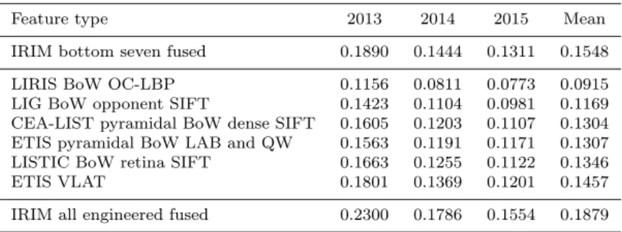
Table 1 Performance of low-level engineered features
Feature type 2013 2014 2015 Mean
IRIM bottom seven fused 0.1890 0.1444 0.1311 0.1548 LIRIS BoW OC-LBP 0.1156 0.0811 0.0773 0.0915 LIG BoW opponent SIFT 0.1423 0.1104 0.0981 0.1169 CEA-LIST pyramidal BoW dense SIFT 0.1605 0.1203 0.1107 0.1304 ETIS pyramidal BoW LAB and QW 0.1563 0.1191 0.1171 0.1307 LISTIC BoW retina SIFT 0.1663 0.1255 0.1122 0.1346 ETIS VLAT 0.1801 0.1369 0.1201 0.1457 IRIM all engineered fused 0.2300 0.1786 0.1554 0.1879
Table 1 shows the performance of several types of engineered features. Performance is shown for the six best groups of feature types as well as the fusion of the seven less good ones and the overall fusion. In several cases, the result is shown for already a combination of variants of the same feature type, for instance corresponding to a pyramidal image decomposition. Performance is given as the Mean (Inferred) Average Precision on the 2013, 2014 and 2015 editions of the TRECVid SIN task as well as their mean. The task was a bit harder in 2014 than in 2013 and a bit harder too in 2015 than in 2014 because the set of evaluated concepts was different, including more difficult ones. We can see that the fusion of all features does significantly better than the best of them. Also, fusion of the seven least performing IRIM feature types does slightly better that the best individual one.
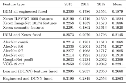
Table 2 Performance engineered and learned features
Feature type 2013 2014 2015 Mean IRIM all engineered fused 0.2300 0.1786 0.1554 0.1879 Xerox ILSVRC 1000 features 0.2190 0.1749 0.1539 0.1824 Xerox ImageNet 10174 features 0.2258 0.1839 0.1570 0.1886 Xerox semantic features 0.2291 0.1862 0.1613 0.1920 IRIM and Xerox fused 0.2573 0.2070 0.1793 0.2145 AlexNet conv5 0.2214 0.1781 0.1610 0.1868 AlexNet fc6 0.2330 0.2001 0.1751 0.2027 AlexNet fc7 0.2277 0.1968 0.1717 0.1985 AlexNet out 0.2114 0.1925 0.1703 0.1910 GoogLeNet pool5 0.2633 0.2234 0.2062 0.2309 VGG-19 out 0.2550 0.2283 0.2042 0.2291 Learned (DCNN) features fused 0.2995 0.2637 0.2350 0.2660 Engineered and DCNN fused 0.3190 0.2849 0.2553 0.2863
Table 2 shows the performance of engineered and learned features as well as of their combinations. The first row reproduces the result of the fusion of all the IRIM engineered features from table 1. The next three rows show the performance of the two Xerox semantic features as well as their fusion. Both have a performance similar to the performance of the fusion of all IRIM features and their fusion has an even higher performance. The Xerox semantic features are very good thanks to their state-of-the-art use of Fisher vectors and to their training on ImageNet data from which the other IRIM features did not benefit from. The next row shows the performance of the fusion of IRIM and Xerox features which is significantly higher than that of each of them taken separately. This performance is the best one that could be achieved using only engineered features (as Xerox ones also fall in this category even though they include some learning).
The next six row of table 2 show the performance obtained with the fea-tures extracted from the AlexNet, GoogLeNet and VGG deep neural networks. It is detailed for the four last layers in the case of AlexNet. The best DCNN feature for each of the three network already has a performance comparable to the IRIM/Xerox fusion or even higher. Again, this is due to the use of Im-ageNet data but also to the very good effectiveness of DCNNs. The last but one row shows the performance of the fusion of the best three DCNN features which is significantly higher than that of each of them taken separately, in-dicating that the three network extract complementary information. Finally, the last row shows the performance of the fusion of non-DCNN-based features and of DCNN-based features. This performance is once again significantly higher than that of both of them taken separately, even if the performance of non-DCNN-based features is significantly lower than that of DCNN-based features, indicating that engineered features are still useful, even with a lower performance.
4.2 Partial DCNN retraining versus use of DCNN layer output as features We made several trials for retraining the last layers of the pre-trained AlexNet, GoogLeNet and VGG-19 implementation using the caffe framework. We tried to retrain the last one, last two or last three layers, doing our best to select the optimal training parameters in each case. Actually, due to the design of the inception module in the GoogLeNet architecture, it was not easy to retrain only the last two or last three layers so, alternatively, we did the two layers retraining by adding another last fully connected layer and we did not try a three layers retraining or any equivalent. The best performance was obtained by cross-validation when retraining only the last two layers for AlexNet and only the last layer for GoogLeNet and VGG-19.
For these features, we were able to do the evaluation both using only one key frame per shot and using additionally all the available I-frames within the shot. In both cases, the training was done using only the key frames as the collaborative annotation was done mostly only on them while the assessment for the evaluation was done on the basis of the full shots [19].
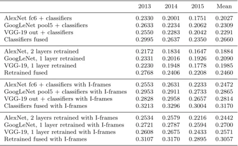
Table 3 shows the performance obtained with the AlexNet, GoogLeNet and VGG-19 implementations as well as for the fusion of their predictions. The first (resp. second) half of the table shows results using only the key frames (resp. using the key frames and the I-frames) for the prediction. Results are displayed using the classical KNN/MSVM learning approach applied to the best extracted features for each implementation and by retraining these implementations. It can be observed that:
• the classical KNN/MSVM learning consistently perform better than the retraining of the last layers. This may be because the last layers actually implement only a one or two-layer perceptron, because there is not enough training data for a good neural network learning (while KNN and MSVM
Table 3 Partial DCNN retraining versus use of DCNN layer outputs as features 2013 2014 2015 Mean AlexNet fc6 + classifiers 0.2330 0.2001 0.1751 0.2027 GoogLeNet pool5 + classifiers 0.2633 0.2234 0.2062 0.2309 VGG-19 out + classifiers 0.2550 0.2283 0.2042 0.2291 Classifiers fused 0.2995 0.2637 0.2350 0.2660 AlexNet, 2 layers retrained 0.2172 0.1834 0.1647 0.1884 GoogLeNet, 1 layer retrained 0.2331 0.2016 0.1926 0.2090 VGG-19, 1 layer retrained 0.2230 0.1948 0.1778 0.1985 Retrained fused 0.2768 0.2406 0.2208 0.2460 AlexNet fc6 + classifiers with I-frames 0.2553 0.2631 0.2233 0.2472 GoogLeNet pool5 + classifiers with I-frames 0.2953 0.2911 0.2733 0.2865 VGG-19 out + classifiers with I-frames 0.2828 0.2958 0.2657 0.2814 Classifiers fused with I-frames 0.3213 0.3296 0.3004 0.3170 AlexNet, 2 layers retrained with I-frames 0.2534 0.2579 0.2216 0.2442 GoogLeNet, 1 layer retrained with I-frames 0.2721 0.2787 0.2594 0.2700 VGG-19, 1 layer retrained with I-frames 0.2608 0.2675 0.2433 0.2571 Retrained fused with I-frames 0.3107 0.3170 0.2895 0.3057
are more robust to this) and/or because they have difficulties with highly imbalanced training data (cost sensitive training was also tried but brought no improvement);
• the differences between 2013, 2014 and 2015 collections and between using or not I-frames are smaller in the case of retrained networks, indicating a better generalization capability despite a lower global performance.
4.3 Combining with improvement methods
Considering the same features, classifiers and fusion methods, several methods can be used to further improve the overall system performance. We evaluated the three following ones: the temporal re-scoring method proposed by Safadi et al. [26], the conceptual feedback method proposed by Hamadi et al. [11], and the use of multiple frames proposed by Snoek et al. [35].
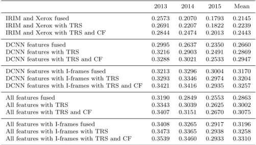
As previously mentioned, only a few of the IRIM engineered features were computed by the participants on the I-frame set; the Xerox features were not available either on this set. Therefore, we were not able to evaluate and compare all the combinations and some fusions are partial. Table 4 shows the effect of the temporal re-scoring (TRS) and conceptual feedback (CF) methods for the fusions of the engineered (IRIM and Xerox) features, the DCNN-based features and their combinations (All). The effect of additionally using the I-frames si also shown, except in the case of the engineered features since not enough of them were available for doing better that using the key frames alone. These were however included in the “All” fusion when possible. It can be observed that:
Table 4 Effect of improvement methods: temporal re-scoring (TRS), conceptual feedback (CF) and use of multiple frames (I-frames)
2013 2014 2015 Mean IRIM and Xerox fused 0.2573 0.2070 0.1793 0.2145 IRIM and Xerox with TRS 0.2691 0.2207 0.1822 0.2239 IRIM and Xerox with TRS and CF 0.2844 0.2474 0.2013 0.2443 DCNN features fused 0.2995 0.2637 0.2350 0.2660 DCNN features with TRS 0.3216 0.2903 0.2491 0.2869 DCNN features with TRS and CF 0.3288 0.3021 0.2533 0.2947 DCNN features with I-frames fused 0.3213 0.3296 0.3004 0.3170 DCNN features with I-frames with TRS 0.3293 0.3346 0.2974 0.3204 DCNN features with I-frames with TRS and CF 0.3421 0.3416 0.2935 0.3257 All features fused 0.3190 0.2849 0.2553 0.2863 All features with TRS 0.3343 0.3039 0.2625 0.3002 All features with TRS and CF 0.3407 0.3151 0.2670 0.3075 All features with I-frames fused 0.3408 0.3265 0.2917 0.3196 All features with I-frames with TRS 0.3473 0.3365 0.2938 0.3258 All features with I-frames with TRS and CF 0.3539 0.3460 0.2933 0.3310
• all three improvement methods are always effective, even when combined though the “TRS” and “I-frames” ones do not accumulate well; this is prob-ably because both search information in the neighborhood, either within the current shot or within adjacent shots and such information may be redundant;
• fusing engineered features and DCNN-based features always lead to an improvement, even if engineered ones are less good and even if less of them were available in the I-frames case.
The five combinations with TRS and CF were the LIG (or Quaero) official sub-missions with respective identifiers: 2C M A Quaero.13 1, 2C M D LIG.15 4, 2C M D LIG.15 2, 2C M D LIG.15 3 and 2C M D LIG.15 1. For the 2015 is-sue of the semantic indexing task, the best MAP was of 0.3624. However, the participant that obtained this result used additional annotations that were not shared with other TRECVid participants. The following participants, ranked second, third and fourth, obtained best MAPs of 0.3086, 0.2987 and 0.2947. Our submission 2C M D LIG.15 1 ranked us as fifth with a MAP of 0.2933. The fourth participant was the IRIM group that used a submission very close to our 2C M D LIG.15 1 one (differing only in the last level of late fusion).
5 Evaluation on the VOC 2012 object classification task
We tried the DCNN features and KNN/MSVM combination on the VOC 2012 classification competition. The official deadline for this competition has passed but the annotations on the test set is kept hidden and an evaluation server is left permanently opened, allowing for new participation in conditions similar
to those of the original competition. The submission count is limited so that no tuning on the test set is possible. The goal of the task is, for each of twenty predefined classes, predict the presence/absence of an example of that class in the test image. More generally, a classification with a real value is expected, allowing to sort the test samples according to their likeliness of containing an example of the target class. The official metric is the average precision (AP) by concept and the overall mean average precision (MAP) over the 20 target classes [8].
We participated with a single submission. We used a single feature for the KNN/MSVM classification. This feature is an early fusion of the AlexNet fc6 layer output (last but two layer, 4096 dimensions), the GoogLeNet pool5 out-put (last but one layer, 1024 dimensions), and the final outout-put of the VGG-19 network (1000 dimensions). These are the same as those used in the TRECVid semantic indexing task, and the same feature optimization 3.4 parameters were used, reducing the dimensionality of the DCNN features to 662, 660 and 609 respectively. Early fusion is then performed by concatenating the three opti-mized and normalized features resulting in a unique feature of 1931 dimensions. A second feature optimization step is performed reducing it further to 294 di-mensions. This is done again with the same parameters as those computed for the TRECVid semantic indexing task. No feature optimization was performed on the VCO 2012 data.
The KNN and MSVM classifiers were trained only using the training and validation data and annotations. No other data and annotation was used di-rectly in the training. ImageNet data and annotations was used indidi-rectly for training the DCNN systems from which the features were extracted and TRECVid SIN data and annotations was used indirectly for optimizing these features and their early fusion but these data and annotations were not used directly for training the classifiers on the VOC 2012 data. Therefore, we made our submission in the “comp1” category as other teams did in similar con-ditions. This submission obtained a MAP of 85.4% while the second best performance obtained a MAP of 82.9%.
6 Conclusion
In this paper, we have compared the use of “traditional” engineered features and learned features for content-based semantic indexing of video documents. We made an extensive comparison of the performance of learned features with traditional engineered ones as well as with combinations of them. Comparison was made in the context of the TRECVid semantic indexing task. Our results confirm those obtained for still images: features learned from other training data generally outperform engineered features for concept recognition. Ad-ditionally, we found that directly training KNN and MSVM classifiers using these features does better than partially retraining the DCNN for adapting it to the new data. We found that, even though the learned features performed
better that the engineered ones, the fusion of both of them still perform sig-nificantly better, indicating that engineered features are still useful, at least in this case. We also found that the improvement methods based on temporal re-scoring, on conceptual feedback and on the use of multiple frames per shot are effective on both types of features and on their combination. Finally, we applied the combination of DCNN features with KNN and MSVM classifiers to the VOC 2012 object classification task where it currently obtains the best performance with a MAP of 85.4%.
Acknowledgements This work was conducted as a part of the CHIST-ERA CAMOMILE project, which was funded by the ANR (Agence Nationale de la Recherche, France). Part of the computations presented in this paper were performed using the Froggy platform of the CIMENT infrastructure (https://ciment.ujf-grenoble.fr), which is supported by the Rhˆone-Alpes region (GRANT CPER07 13 CIRA) and the Equip@Meso project (reference ANR-10-EQPX-29-01) of the programme Investissements d’Avenir supervised by the Agence Nationale pour la Recherche. Results from the IRIM network were also used in these exper-iments [4]. The authors also wish to thank Florent Perronnin from XRCE for providing fea-tures based on classification scores from classifiers trained on ILSVRC/ImageNet data [28].
References
1. Ayache, S., Qu´enot, G.: Video Corpus Annotation using Active Learning. In: European Conference on Information Retrieval (ECIR), pp. 187–198. Glasgow, Scotland (2008) 2. Ayache, S., Qu´enot, G., Gensel, J.: Image and video indexing using networks of
op-erators. EURASIP Journal on Image and Video Processing 2007(1), 056,928 (2007). DOI 10.1155/2007/56928
3. Benoit, A., Caplier, A., Durette, B., Herault, J.: Using human visual system modeling for bio-inspired low level image processing. Computer Vision and Image Understanding 114(7), 758 – 773 (2010). DOI http://dx.doi.org/10.1016/j.cviu.2010.01.011
4. Borgne, H.L., Gosselin, P., Picard, D., Redi, M., M´erialdo, B., Mansencal, B., Benois-Pineau, J., Ayache, S., Hamadi, A., Safadi, B., Derbas, N., Budnik, M., Qu´enot, G., Gao, B., Zhu, C., Tang, Y., Dellandrea, E., Bichot, C.E., Chen, L., Benoit, A., Lambert, P., Strat, T.: IRIM at TRECVid 2015: Semantic Indexing. In: Proceedings of TRECVID 2015. NIST, USA (2015)
5. Chatfield, K., Simonyan, K., Vedaldi, A., Zisserman, A.: Return of the devil in the details: Delving deep into convolutional nets. CoRR abs/1405.3531 (2014)
6. Csurka, G., Bray, C., Dance, C., Fan, L.: Visual categorization with bags of keypoints. In: Workshop on Statistical Learning in Computer Vision, ECCV, pp. 1–22 (2004) 7. Deng, J., Dong, W., Socher, R., Li, L.J., Li, K., Fei-Fei, L.: ImageNet: A Large-Scale
Hierarchical Image Database. In: CVPR09 (2009)
8. Everingham, M., Eslami, S.M.A., Van Gool, L., Williams, C.K.I., Winn, J., Zisserman, A.: The pascal visual object classes challenge: A retrospective. International Journal of Computer Vision 111(1), 98–136 (2015)
9. Fukushima, K.: Neocognitron: A self-organizing neural network model for a mechanism of pattern recognition unaffected by shift in position. Biological Cybernetics 36, 193–202 (1980)
10. Gosselin, P.H., Cord, M., Philipp-Foliguet, S.: Combining visual dictionary, kernel-based similarity and learning strategy for image category retrieval. Com-puter Vision and Image Understanding 110(3), 403 – 417 (2008). DOI http://dx.doi.org/10.1016/j.cviu.2007.09.018. Similarity Matching in Computer Vision and Multimedia
11. Hamadi, A., Mulhem, P., Qu´enot, G.: Extended conceptual feedback for semantic mul-timedia indexing. Mulmul-timedia Tools and Applications 74(4), 1225–1248 (2015). DOI 10.1007/s11042-014-1937-y
12. Hinton, G.E., Salakhutdinov, R.R.: Reducing the dimensionality of data with neural networks. Science 313(5786), 504–507 (2006). DOI 10.1126/science.1127647. URL http://science.sciencemag.org/content/313/5786/504
13. J´egou, H., Perronnin, F., Douze, M., S´anchez, J., P´erez, P., Schmid, C.: Aggregating local image descriptors into compact codes. IEEE Transactions on Pattern Analysis and Machine Intelligence 34(9), 1704–1716 (2012). DOI 10.1109/TPAMI.2011.235 14. Krizhevsky, A., Sutskever, I., Hinton, G.E.: Imagenet classification with deep
convo-lutional neural networks. In: F. Pereira, C. Burges, L. Bottou, K. Weinberger (eds.) Advances in Neural Information Processing Systems 25, pp. 1097–1105. Curran Asso-ciates, Inc. (2012)
15. LeCun, Y., Bottou, L., Bengio, Y., Haffner, P.: Gradient-based learning applied to document recognition. In: Proceedings of the IEEE, pp. 2278–2324 (1998)
16. Lowe, D.G.: Distinctive image features from scale-invariant keypoints. Int. J. Comput. Vision 60(2), 91–110 (2004). DOI 10.1023/B:VISI.0000029664.99615.94
17. Nair, V., Hinton, G.E.: Rectified linear units improve restricted boltzmann ma-chines. In: J. Frnkranz, T. Joachims (eds.) Proceedings of the 27th International Conference on Machine Learning (ICML-10), pp. 807–814. Omnipress (2010). URL http://www.icml2010.org/papers/432.pdf
18. Orr, G.B., Mueller, K.R. (eds.): Neural Networks : Tricks of the Trade, Lecture Notes in Computer Science, vol. 1524. Springer (1998)
19. Over, P., Awad, G., Michel, M., Fiscus, J., Kraaij, W., Smeaton, A.F., Qu´enot, G., Or-delman, R.: Trecvid 2015 – an overview of the goals, tasks, data, evaluation mechanisms and metrics. In: Proceedings of TRECVID 2015. NIST, USA (2015)
20. Picard, D., Gosselin, P.H.: Efficient image signatures and similarities using tensor prod-ucts of local descriptors. Computer Vision and Image Understanding 117(6), 680–687 (2013). DOI 10.1016/j.cviu.2013.02.004
21. Razavian, A., Azizpour, H., Sullivan, J., Carlsson, S.: CNN Features Off-the-Shelf: An Astounding Baseline for Recognition. In: IEEE Conference on Computer Vi-sion and Pattern Recognition Workshops (CVPRW), pp. 512–519 (2014). DOI 10.1109/CVPRW.2014.131
22. Russakovsky, O., Deng, J., Su, H., Krause, J., Satheesh, S., Ma, S., Huang, Z., Karpathy, A., Khosla, A., Bernstein, M., Berg, A.C., Fei-Fei, L.: ImageNet Large Scale Visual Recognition Challenge. International Journal of Computer Vision (IJCV) pp. 1–42 (2015). DOI 10.1007/s11263-015-0816-y
23. Safadi, B., Derbas, N., Hamadi, A., Budnik, M., Mulhem, P., Qu´enot, G.: LIG at TRECVid 2015: Semantic Indexing. In: Proceedings of TRECVID. Orlando, United States (2014)
24. Safadi, B., Derbas, N., Qu´enot, G.: Descriptor optimization for multimedia indexing and retrieval. Multimedia Tools and Applications 74(4), 1267–1290 (2015). DOI 10.1007/s11042-014-2071-6
25. Safadi, B., Qu´enot, G.: Evaluations of multi-learner approaches for concept in-dexing in video documents. In: Adaptivity, Personalization and Fusion of Het-erogeneous Information, RIAO ’10, pp. 88–91. Le centre de hautes ´etudes in-ternationales d’informatique documentaire, Paris, France, France (2010). URL http://dl.acm.org/citation.cfm?id=1937055.1937075
26. Safadi, B., Qu´enot, G.: ranking by Local scoring for Video Indexing and Re-trieval. In: I.R. Craig Macdonald Iadh Ounis (ed.) CIKM 2011 - International Con-ference on Information and Knowledge Management, pp. 2081–2084. ACM, Glasgow, United Kingdom (2011). DOI 10.1145/2063576.2063895. Poster session: information retrieval
27. Safadi, B., Qu´enot, G.: A factorized model for multiple svm and multi-label classification for large scale multimedia indexing. In: Content-Based Multimedia Indexing (CBMI), 2015 13th International Workshop on, pp. 1–6 (2015). DOI 10.1109/CBMI.2015.7153610 28. S´anchez, J., Perronnin, F., Mensink, T., Verbeek, J.: Image classification with the fisher vector: Theory and practice. International journal of computer vision 105(3), 222–245 (2013)
29. van de Sande, K.E.A., Gevers, T., Snoek, C.G.M.: Evaluating color descriptors for object and scene recognition. IEEE Transactions on Pattern Analysis and Machine Intelligence 32(9), 1582–1596 (2010)
30. Shabou, A., LeBorgne, H.: Locality-constrained and spatially regularized coding for scene categorization. In: Computer Vision and Pattern Recognition (CVPR), 2012 IEEE Conference on, pp. 3618–3625 (2012). DOI 10.1109/CVPR.2012.6248107 31. Simonyan, K., Zisserman, A.: Very deep convolutional networks for large-scale image
recognition. CoRR abs/1409.1556 (2014). URL http://arxiv.org/abs/1409.1556 32. Sivic, J., Zisserman, A.: Video google: A text retrieval approach to object matching
in videos. In: Proceedings of the Ninth IEEE International Conference on Computer Vision - Volume 2, ICCV ’03, pp. 1470–. IEEE Computer Society, Washington, DC, USA (2003)
33. Smeaton, A.F., Over, P., Kraaij, W.: Evaluation campaigns and trecvid. In: MIR ’06: Proceedings of the 8th ACM International Workshop on Multimedia Infor-mation Retrieval, pp. 321–330. ACM Press, New York, NY, USA (2006). DOI http://doi.acm.org/10.1145/1178677.1178722
34. Smith, J., Naphade, M., Natsev, A.: Multimedia semantic indexing using model vectors. In: Multimedia and Expo, 2003. ICME ’03. Proceedings. 2003 International Conference on, vol. 2, pp. II–445–8 vol.2 (2003). DOI 10.1109/ICME.2003.1221649
35. Snoek, C.G.M., Worring, M., Geusebroek, J.M., Koelma, D.C., Seinstra, F.J.: On the surplus value of semantic video analysis beyond the key frame. In: IEEE International Conference on Multimedia & Expo (2005). URL https://ivi.fnwi.uva.nl/isis/publications/2005/SnoekICME2005
36. Strat, S., Benoit, A., Lambert, P.: Retina enhanced sift descriptors for video indexing. In: Content-Based Multimedia Indexing (CBMI), 2013 11th International Workshop on, pp. 201–206 (2013). DOI 10.1109/CBMI.2013.6576582
37. Strat, S., Benoit, A., Lambert, P.: Retina enhanced bag of words descriptors for video classification. In: Signal Processing Conference (EUSIPCO), 2014 Proceedings of the 22nd European, pp. 1307–1311 (2014)
38. Strat, S.T., Benoit, A., Lambert, P., Bredin, H., Qu´enot, G.: Hierarchical late fusion for concept detection in videos. In: B. Ionescu, J. Benois-Pineau, T. Piatrik, G. Qu´enot (eds.) Fusion in Computer Vision, Advances in Computer Vision and Pattern Recog-nition, pp. 53–77. Springer International Publishing (2014). DOI 10.1007/978-3-319-05696-8 3. URL http://dx.doi.org/10.1007/978-3-319-10.1007/978-3-319-05696-8 3
39. Su, Y., Jurie, F.: Improving image classification using semantic attributes. International Journal of Computer Vision 100(1), 59–77 (2012). DOI 10.1007/s11263-012-0529-4 40. Szegedy, C., Liu, W., Jia, Y., Sermanet, P., Reed, S., Anguelov, D., Erhan, D.,
Van-houcke, V., Rabinovich, A.: Going deeper with convolutions. CoRR abs/1409.4842 (2014). URL http://arxiv.org/abs/1409.4842
41. Yosinski, J., Clune, J., Bengio, Y., Lipson, H.: How transferable are features in deep neural networks? CoRR abs/1411.1792 (2014)
42. Zhu, C., Bichot, C.E., Chen, L.: Color orthogonal local binary patterns combination for image region description. Rapport technique RR-LIRIS-2011-012, LIRIS UMR 5205, 15 (2011)