HAL Id: hal-00926178
https://hal.inria.fr/hal-00926178
Submitted on 9 Jan 2014
HAL is a multi-disciplinary open access
archive for the deposit and dissemination of
sci-entific research documents, whether they are
pub-lished or not. The documents may come from
teaching and research institutions in France or
abroad, or from public or private research centers.
L’archive ouverte pluridisciplinaire HAL, est
destinée au dépôt et à la diffusion de documents
scientifiques de niveau recherche, publiés ou non,
émanant des établissements d’enseignement et de
recherche français ou étrangers, des laboratoires
publics ou privés.
and Algorithms
Anne Benoit, Umit Catalyurek, Yves Robert, Erik Saule
To cite this version:
Anne Benoit, Umit Catalyurek, Yves Robert, Erik Saule. A Survey of Pipelined Workflow Scheduling:
Models and Algorithms. ACM Computing Surveys, Association for Computing Machinery, 2013, 45
(4), �10.1145/2501654.2501664�. �hal-00926178�
Models and Algorithms
ANNE BENOIT ´
Ecole Normale Sup´erieure de Lyon, France
and ¨
UM˙IT V. C¸ ATALY ¨UREK
Department of Biomedical Informatics and Department of Electrical & Computer En-gineering, The Ohio State University
and
YVES ROBERT ´
Ecole Normale Sup´erieure de Lyon, France & University of Tennessee Knoxville and
ERIK SAULE
Department of Biomedical Informatics, The Ohio State University
A large class of applications need to execute the same workflow on different data sets of identical size. Efficient execution of such applications necessitates intelligent distribution of the application components and tasks on a parallel machine, and the execution can be orchestrated by utilizing task-, data-, pipelined-, and/or replicated-parallelism. The scheduling problem that encompasses all of these techniques is called pipelined workflow scheduling, and it has been widely studied in the last decade. Multiple models and algorithms have flourished to tackle various programming paradigms, constraints, machine behaviors or optimization goals. This paper surveys the field by summing up and structuring known results and approaches.
Categories and Subject Descriptors: F.2.2 [Nonnumerical Algorithms and Problems]: Se-quencing and scheduling; C.1.4 [Parallel Architectures ]: Distributed architectures
General Terms: Algorithms, Performance, Theory
Additional Key Words and Phrases: workflow programming, filter-stream programming, schedul-ing, pipeline, throughput, latency, models, algorithms, distributed systems, parallel systems
Authors’ Address: Anne Benoit and Yves Robert, Laboratoire de l’Informatique du Parall´elisme, ´
Ecole Normale Sup´erieure de Lyon, 46 All´ee d’Italie 69364 LYON Cedex 07, FRANCE, {Anne.Benoit|Yves.Robert}@ens-lyon.fr.
¨
Umit V. C¸ ataly¨urek and Erik Saule, The Ohio State University, 3190 Graves Hall — 333 W. Tenth Ave., Columbus, OH 43210, USA, {umit|esaule}@bmi.osu.edu.
Permission to make digital/hard copy of all or part of this material without fee for personal or classroom use provided that the copies are not made or distributed for profit or commercial advantage, the ACM copyright/server notice, the title of the publication, and its date appear, and notice is given that copying is by permission of the ACM, Inc. To copy otherwise, to republish, to post on servers, or to redistribute to lists requires prior specific permission and/or a fee.
c
1. INTRODUCTION
For large-scale applications targeted to parallel and distributed computers, finding an efficient task and communication mapping and schedule is critical to reach the best possible application performance. At the heart of the scheduling process is a graph, the workflow, of an application: an abstract representation that expresses the atomic computation units and their data dependencies. Hence, the application is partitioned into tasks that are linked by precedence constraints, and it is described by, usually, a directed acyclic graph (also called DAG), where the vertices are the tasks, and the edges represent the precedence constraints. In classical workflow scheduling techniques, there is a single data set to be executed, and the goal is to minimize the latency or makespan, which corresponds to the total execution time of the workflow, where each task is executed once [KA99b].
The graphical representations are not only used for parallelizing computations. In mid 70s and early 80s, a graphical representation called dataflow [Den74; Dav78; Den80] emerged as a powerful programming and architectural paradigm. Lee and Parks [LP95] present a rigorous formal foundation of dataflow languages, for which they coined the term dataflow process networks and presented it as a special case of Kahn process networks (KPN) [Kah74]. In KPN, a group of deterministic se-quential tasks communicate through unbounded first-in, first-out channels. As a powerful paradigm that implicitely supports parallelism, dataflow networks (hence KPNs) have been used to exploit parallelism at compile time [HL97] and run
time [NTS+08].
With the turn of the new millennium, Grid computing [FKT01] emerged as a global cyber-infrastructure for large-scale, integrative e-Science applications. At the core of Grid computing sit Grid workflow managers that schedule coarse-grain computations onto dynamic Grid resources. Yu and Buyya [YB05] present an excel-lent survey on workflow scheduling for Grid computing. Grid workflow managers, such as DAGMan [TWML01] (of the Condor project [LLM88; TTL02]),
Pega-sus [DShS+05], GrADS [BCC+01], Taverna [OGA+06], and ASKALON [FJP+05],
utilize DAGs and abstract workflow languages for scheduling workflows onto dy-namic Grid resources using performance modeling and prediction systems like Prophesy [TWS03], NWS [WSH99] and Teuta [FPT04]. The main focus of such Grid workflow systems are the discovery and utilization of dynamic resources that span over multiple administrative domains. It involves handling of authentication and authorization, efficient data transfers, and fault tolerance due to the dynamic nature of the systems.
The main focus of this paper is a special class of workflow scheduling that we call pipelined workflow scheduling (or in short pipelined scheduling). Indeed, we focus on the scheduling of applications that continuously operate on a stream of data sets, which are processed by a given wokflow, and hence the term pipelined. In steady-state, similar to dataflow and Kahn networks, data sets are pumped from one task to its successor. These data sets all have the same size, and they might be obtained by
partitioning the input into several chunks. For instance in image analysis [SKS+09],
a medical image is partitioned in tiles, and tiles are processed one after the other. Other examples of such applications include video processing [GRRL05], motion
molecular biology [RKO+03], medical imaging [GRR+06], and various scientific data analyses, including particle physics [DBGK03], earthquake [KGS04], weather
and environmental data analyses [RKO+03].
The pipelined execution model is the core of many software and programming middlewares. It is used on different types of parallel machines such as SMP (Intel
TBB [Rei07]), clusters (DataCutter [BKC¸+01], Anthill [TFG+08], Dryad [IBY+07]),
Grid computing environments (Microsoft AXUM [Mic09], LONI [MGPD+08],
Ke-pler [BML+06]), and more recently on clusters with accelerators (see for instance
DataCutter [HC¸ R+08] and DataCutter-Lite [HC¸ 09]). Multiple models and
algo-rithms have emerged to deal with various programming paradigms, hardware con-straints, and scheduling objectives.
It is possible to reuse classical workflow scheduling techniques for pipelined ap-plications, by first finding an efficient parallel execution schedule for one single data set (makespan minimization), and then executing all the data sets using the same schedule, one after the other. Although some good algorithms are known for such problems [KA99a; KA99b], the resulting performance of the system for a pipelined application may be far from the peak performance of the target parallel platform. The workflow may have a limited degree of parallelism for efficient processing of a single data set, and hence the parallel machine may not be fully utilized. Rather, for pipelined applications, we need to decide how to process multiple data sets in parallel. In other words, pipelined scheduling is dealing with both intra data set and inter data set parallelism (the different types of parallelism are described below in more details). Applications that do not allow the latter kind of parallelism are outside the scope of this survey. Such applications include those with a feedback loop such as iterative solvers. When feedback loops are present, applications are typically scheduled by software pipelining, or by cyclic scheduling techniques (also called cyclic PERT-shop scheduling, where PERT refers to Project Evaluation and Review Technique). A survey on software pipelining can be found in [AJLA95], and on cyclic scheduling in [LKdPC10].
To evaluate the performance of a schedule for a pipelined workflow, various op-timization criteria are used in the literature. The most common ones are (i) the latency (denoted by L), or makespan, which is the maximum time a data set spends in the system, and (ii) the throughput (denoted by T ), which is the number of data sets processed per time unit. The period of the schedule (denoted by P) is the time elapsed between two consecutive data sets entering the system. Note that the period is the inverse of the achieved throughput, hence we will use them inter-changeably. Depending on the application, a combination of multiple performance objectives may be desired. For instance, an interactive video processing application
(such as SmartKiosk [KRC+99], a computerized system that interacts with
multi-ple peomulti-ple using cameras) needs to be reactive while ensuring a good frame rate; these constraints call for an efficient latency/throughput trade-off. Other criteria may include reliability, resource cost, and energy consumption.
Several types of parallelism can be used to achieve good performance. If one task of the workflow produces directly or transitively the input of another task, the two tasks are said to be dependent; otherwise they are independent. Task-parallelism is the most well-known form of parallelism and consists in concurrently executing
independent tasks for the same data set; it can help minimize the workflow latency. Pipelined-parallelism is used when two dependent tasks in the workflow are be-ing executed simultaneously on different data sets. The goal is to improve the throughput of the application, possibly at the price of more communications, hence potentially a larger latency. Pipelined-parallelism was made famous by assembly lines and later reused in processors in the form of the instruction pipeline in CPUs and the graphic rendering pipeline in GPUs.
Replicated-parallelism can improve the throughput of the application, because several copies of a single task operate on different data sets concurrently. This is especially useful in situations where more computational resources than workflow tasks are available. Replicated-parallelism is possible when reordering the pro-cessing of the data sets by one task does not break the application semantics, for instance when the tasks perform a stateless transformation. A simple example of a task allowing replicated-parallelism would be computing the square root of the data set (a number), while computing the sum of the numbers processed so far would be stateful and would not allow replicated-parallelism.
Finally, data-parallelism may be used when some tasks contain inherent paral-lelism. It corresponds to using several processors to execute a single task for a single data set. It is commonly used when a task is implemented by a software library that supports parallelism on its own, or when a strongly coupled parallel execution can be performed.
Note that task-parallelism and data-parallelism are inherited from classical work-flow scheduling, while pipelined-parallelism and replicated-parallelism are only found in pipelined workflow scheduling.
In a nutshell, the main contributions of this survey are the following: (i) proposing a three-tiered model of pipelined workflow scheduling problems; (ii) structuring existing work; and (iii) providing detailed explanations on schedule reconstruction techniques, which are often implicit in the literature.
The rest of this paper is organized as follows. Before going into technical de-tails, Section 2 presents a motivating example to illustrate the various parallelism techniques, task properties, and their impact on objective functions.
The first issue when dealing with a pipelined application is to select the right model among the tremendous number of variants that exist. To solve this issue, Section 3 organizes the different characteristics that the target application can exhibit into three components: the workflow model, the system model, and the performance model. This organization helps position a given problem with respect to related work.
The second issue is to build the relevant scheduling problem from the model of the target application. There is no direct formulation going from the model to the scheduling problem, so we cannot provide a general method to derive the scheduling problem. However, in Section 4, we illustrate the main techniques on basic problems, and we show how the application model impacts the scheduling problem. The scheduling problems become more or less complicated depending upon the application requirements. As usual in optimization theory, the most basic (and sometimes unrealistic) problems can usually be solved in polynomial time, whereas the most refined and accurate models usually lead to NP-hard problems.
Although the complexity of some problems is still open, Section 4 concludes by highlighting the known frontier between polynomial and NP-complete problems.
Finally, in Section 5, we survey various techniques that can be used to solve the scheduling problem, i.e., to find the best parallel execution of the application according to the performance criteria. We provide optimal algorithms to solve the simplest problem instances in polynomial time. For the most difficult instances, we present some general heuristic methods, which aim at giving good approximate solutions.
2. MOTIVATING EXAMPLE
In this section, we focus on a simple pipelined application and emphasize the need for scheduling algorithms.
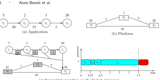
Consider an application composed of four tasks, whose dependencies form a linear
chain: a data set must first be processed by task t1 before it can be processed
by t2, then t3, and finally t4. The computation weights of tasks t1, t2, t3 and t4
(or task weights) are set respectively to 5, 2, 3, and 20, as illustrated in Fig. 1(a). If two consecutive tasks are executed on two distinct processors, then some time is required for communication, in order to transfer the intermediate result. The communication weights are set respectively to 20, 15 and 1 for communications
t1 → t2, t2 → t3, and t3 → t4 (see Fig. 1(a)). The communication weight along
an edge corresponds to the size of the intermediate result that has to be sent from the processor in charge of executing the source task of the edge to the processor in charge of executing the sink task of the edge, whenever these two processors are different. Note that since all input data sets have the same size, the intermediate results when processing different data sets also are assumed to have identical size, even though this assumption may not be true for some applications.
The target platform consists of three processors, with various speeds and
inter-connection bandwidths, as illustrated in Fig. 1(b). If task t1 is scheduled to be
executed on processor P2, a data set is processed within 5
1= 5 time units, while the
execution on the faster processor P1 requires only 5
10 = 0.5 time units (task weight
divided by processor speed). Similarly, the communication of a data of weight c
from processor P1to processor P2takes c
1 time units, while it is ten times faster to
communicate from P1 to P3.
First examine the execution of the application when mapped sequentially on the
fastest processor, P3 (see Fig. 1(c)). For such an execution, there is no
communi-cation. The communication weights and processors that are not used are shaded in grey on the figure. On the right, the processing of the first data set (and the beginning of the second one) is illustrated. Note that because of the dependencies between tasks, this is actually the fastest way to process a single data set. The
latency is computed as L = 5+2+3+2020 = 1.5. A new data set can be processed once
the previous one is finished, hence the period P = L = 1.5.
Of course, this sequential execution does not exploit any parallelism. Since there are no independent tasks in this application, we cannot use task-parallelism here. However, we now illustrate pipelined-parallelism: different tasks are scheduled on distinct processors, and thus they can be executed simultaneously on different data sets. In the execution of Fig. 1(d), all processors are used, and we greedily balance
1 5 2 3 20 20 15 t1 t2 t3 t4 (a) Application. 5 10 1 20 10 1 P2 P1 P3 (b) Platform. 1 processor 3 time 0 0.25 0.5 1.5 10 1 20 10 1 5 5 2 3 20 20 15 1 t1 t2 t3 t4 P1 P2 P3 t1 t2 t3 t4
(c) Sequential execution on the fastest processor.
0.5 1 10 1 5 5 2 3 20 20 15 11 10 20 0 processor 2 20.5 1 3 time 38.9 37.9 37.8 22.5 37.5 P1 P2 P3 t1 t2 t3 t4 t1 t2 t3 t4
(d) Greedy execution using all processors.
3 1 10 1 5 5 2 3 20 20 15 11 10 20 time 0 0.5 1 processor 1 22.1 3 P1 P2 P3 t1 t2 t3 t4 t1 t2 t3 t4
(e) Resource selection to optimize period. Fig. 1. Motivating example.
the computation requirement of tasks according to processor speeds. The perfor-mance of such a parallel execution turns out to be quite bad, because several large communications occur. The latency is now obtained by summing up all
computa-tion and communicacomputa-tion times: L = 105 + 20 + 2 + 15 + 103 + 101 +2020 = 38.9, as
illustrated on the right of the figure for the first data set. Moreover, the period is not better than the one obtained with the sequential execution presented pre-viously, because communications become the bottleneck of the execution. Indeed,
the transfer from t1 to t2 takes 20 time units, and therefore the period cannot be
better than 20: P ≥ 20. This example of execution illustrates that parallelism should be used with caution.
However, one can obtain a period better than that of the sequential execution as shown in Fig. 1(e). In this case, we enforce some resource selection: the slowest
processor P2is discarded (in grey) since it only slows down the whole execution. We
process different data sets in parallel (see the execution on the right): within one
unit of time, we can concurrently process one data set by executing t4 on P3, and
another data set by executing t1, t2, t3(sequentially) on P1. This partially sequential execution avoids all large communication weights (in grey). The communication
time corresponds only to the communication between t3 and t4, from P1 to P3,
and it takes a time 1
10. We assume that communication and computation can
overlap when processing distinct data sets, and therefore, once the first data set
has been processed (at time 1), P1can simultaneously communicate the data to P3
and start computing the second data set. Finally, the period is P = 1. Note that this improved period is obtained at the price of a higher latency: the latency has
increased from 1.5 in the fully sequential execution to L = 1 +101 + 1 = 2.1 here.
This example illustrates the necessity of finding efficient trade-offs between an-tagonistic criteria.
3. MODELING TOOLS
This section gives general information on the various scheduling problems. It should help the reader understand the key properties of pipelined applications.
All applications of pipelined scheduling are characterized by properties from three components that we call the workflow model, the system model and the performance model. These components correspond to “which kind of program we are schedul-ing”, “which parallel machine will host the program”, and “what are we trying to optimize”. This three-component view is similar to the three-field notation used to define classical scheduling problems [Bru07].
In the example of Section 2, the workflow model is an application with four tasks arranged as a linear chain, with computation and communication weights; the system model is a three-processor platform with speeds and bandwidths; and the performance model corresponds to the two optimization criteria, latency and period. We present in Sections 3.1, 3.2 and 3.3 the three models; then Section 3.4 classifies work in the taxonomy that has been detailed.
3.1 Workflow Model
The workflow model defines the program that is going to be executed; its compo-nents are presented in Fig. 2.
As stated in the introduction, programs are usually represented as Directed Acyclic Graphs (DAGs) in which nodes represent computation tasks, and edges represent dependencies and/or communications between tasks. The shape of the graph is a parameter. Most program DAGs are not arbitrary but instead have some predefined form. For instance, it is common to find DAGs that are a single linear chain, as in the example of Section 2. Some other frequently encountered structures are fork graphs (for reduce operations), trees (in arithmetic expression evaluation; for instance in database [HM94]), fork-join, and series-parallel graphs (commonly
found when using nested parallelism [BHS+94]). The DAG is sometimes extended
with two zero-weight nodes, a source node, which is made a predecessor of all entry nodes of the DAG, and a sink node, which is made a successor of all exit nodes of
Workflow Model Shape Task Weight Comm. Weight Task Parellelism Task Execution sequential, parallel Linear chain, fork, tree,
fork-join, series-parallel, general DAG
unit, non-unit 0 (precedence only),unit, non-unit monolithic, replicable
Fig. 2. The components of the workflow model.
the DAG. This construction is purely technical and allows for faster computation of dependence paths in the graph.
The weight of the tasks are important because they represent computation re-quirements. For some applications, all the tasks have the same computation require-ment (they are said to be unit tasks). The weight of communications is defined similarly, it usually corresponds to the size of the data to be communicated from one task to another, when mapped on different processors. Note that a zero weight may be used to express a precedence between tasks, when the time to communicate can be ignored.
The tasks of the program may themselves contain parallelism. This adds a level of parallelism to the execution of the application, that is called data-parallelism. Although the standard model only uses sequential tasks, some applications feature parallel tasks. Three models of parallel tasks are commonly used (this naming was
proposed by [FRS+97] and is now commonly used in job scheduling for production
systems): a rigid task requires a given number of processors to execute; a moldable task can run on any number of processors, and its computation time is given by a speed-up function (that can either be arbitrary, or match a classical model such as the Amdahl’s law [Amd67]); and a malleable task can change the number of processors it is executing on during its execution.
The task execution model indicates whether it is possible to execute concurrent replicas of a task at the same time or not. Replicating a task may not be possible due to an internal state of the task; the processing of the next data set depends upon the result of the computation of the current one. Such tasks are said to be monolithic; otherwise they are replicable. When a task is replicated, it is common to impose some constraints on the allocation of the data sets to the replicas. For instance, the dealable stage rule [Col04] forces data sets to be allocated in a round-robin fashion among the replicas. This constraint is enforced to avoid out-of-order completion and is quite useful when, say, a replicated task is followed by a monolithic one.
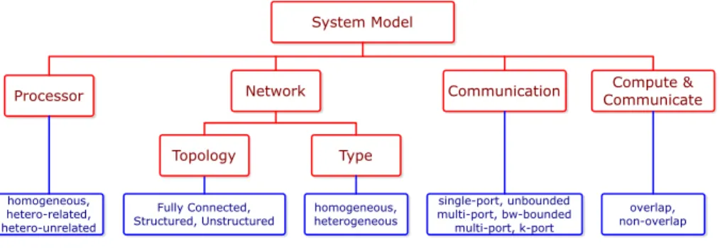
3.2 System Model
The system model describes the parallel machine used to run the program; its components are presented in Fig. 3 and are now described in more details.
First, processors may be identical (homogeneous), or instead they can have dif-ferent processing capabilities (heterogeneous). There are two common models of heterogeneous processors. Either their processing capabilities are linked by a con-stant factor, i.e., the processors have different speeds (known as the related model in scheduling theory and sometimes called heterogeneous uniform), or they are not
System Model
Processor Network Communication
homogeneous, hetero-related, hetero-unrelated Fully Connected, Structured, Unstructured single-port, unbounded multi-port, bw-bounded multi-port, k-port Topology Type homogeneous, heterogeneous Compute & Communicate overlap, non-overlap
Fig. 3. The components of the system model.
speed-related, which means that a processor may be fast on a task but slow on another one (known as the unrelated model in scheduling theory and sometimes called completely heterogeneous). Homogeneous and related processors are com-mon in clusters. Unrelated processors arise when dealing with dedicated hardware or from preventing certain tasks to execute on some machines (to handle licensing issues or applications that do not fit in some machine memory). This decomposition in three models is classical in the scheduling literature [Bru07].
The network defines how the processors are interconnected. The topology of the network describes the presence and capacity of the interconnection links. It is common to find fully connected networks in the literature, which can model buses as well as Internet connectivity. Arbitrary networks whose topologies are specified explicitly through an interconnection graph are also common. In between, some systems may exhibit structured networks such as chains, 2D-meshes, 3D-torus, etc. Regardless of the connectivity of the network, links may be of different types. They can be homogeneous – transport the information in the same way – or they can have different speeds. The most common heterogeneous link model is the bandwidth model, in which a link is characterized by its sole bandwidth. There exist other communication models such as the delay model [RS87], which assumes that all the communications are completely independent. Therefore, the delay model does not require communications to be scheduled on the network but only requires the processors to wait for a given amount of time when a communication is required. Frequently, the delay between two tasks scheduled on two different processors is computed based on the size of the message and the characteristics (latency and bandwidth) of the link between the processors. The LogP (Latency, overhead, gap
and Processor) model [CKP+93] is a realistic communication model for fixed size
messages. It takes into account the transfer time on the network, the latency of the network and the time required by a processor to prepare the communication. The LogGP model [AISS95] extends the LogP model by taking the size of the message into account using a linear model for the bandwidth. The latter two models are seldom used in pipelined scheduling.
Some assumptions must be made in order to define how communications take place. The one-port model [BRP03] forbids a processor to be involved in more than one communication at a time. This simple, but somewhat pessimistic, model is useful for representing single-threaded systems; it has been reported to accurately
model certain MPI implementations that serialize communications when the mes-sages are larger than a few megabytes [SP04]. The opposite model is the multi-port model that allows a processor to be involved in an arbitrary number of communi-cations simultaneously. This model is often considered to be unrealistic since some algorithms will use a large number of simultaneous communications, which induces large overheads in practice. An in-between model is the k-port model where the number of simultaneous communications must be bounded by a parameter of the problem [HP03]. In any case, the model can also limit the total bandwidth that a node can use at a given time (that corresponds to the capacity of its network card). Finally, some machines have hardware dedicated to communication or use multi-threading to handle communication; thus they can compute while using the net-work. This leads to an overlap of communication and computation, as was assumed in the example of Section 2. However, some machines or software libraries are still mono-threaded, and then such an overlapping is not possible.
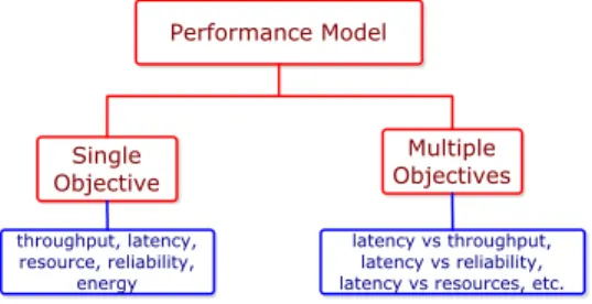
3.3 Performance Model
The performance model describes the goal of the scheduler and tells from two valid schedules which one is better. Its components are presented in Fig. 4.
The most common objective in pipelined scheduling is to maximize the through-put of the system, which is the number of data sets processed per time unit. In permanent applications such as interactive real time systems, it indicates the load that the system can handle. Recall that this is equivalent to minimizing the period, which is the inverse of the throughput.
Another common objective is to minimize the latency of the application, which is basically defined as the time taken by a single data set to be entirely processed. It measures the response time of the system to handle each data set. The objective chosen to measure response time is most of the time the maximum latency, since the latency of different data sets may be different. Latency is mainly relevant in interactive systems. Note that latency minimization corresponds to makespan minimization in DAG scheduling, when there is a single data set to process.
Other objectives have also been studied. When the size of the computing system increases, hardware and software become more likely to be affected by malfunctions.
There are many formulations of this problem (see [BBG+09] for details), but most
of the time it reduces to optimizing the probability of correct execution of the application, which is called the reliability of the system [GST09]. Another objective function that is extensively studied is the energy consumption, which has recently
Performance Model Single Objective Multiple Objectives throughput, latency, resource, reliability, energy latency vs throughput, latency vs reliability, latency vs resources, etc.
become a critical problem, both for economic and environmental reasons [Mil99]. It is often assumed that the speed of processors can be dynamically adjusted [JPG04; WvLDW10], and the slower a processor is, the less energy it consumes. Different models exist, but the main parameters are how the energy cost is computed from the speed (the energy cost is usually quadratic or cubic in the speed) and whether possible speeds are given by a continuous interval [YDS95; BKP07] or by a discrete set of values [OYI01; Pra04].
The advent of more complex systems and modern user requirements increased the interest in the optimization of several objectives at the same time. There are various ways to optimize multiple objectives [DRST09], but the most classical one is to optimize one of the objectives while ensuring a given threshold value on the other ones. Deciding which objectives are constrained, and which one remains to opti-mize, makes no theoretical difference [TB07]. However, there is often an objective that is a more natural candidate for optimization when designing heuristics.
3.4 Placing Related Work in the Taxonomy
The problem of scheduling pipelined linear chains, with both monolithic and repli-cable tasks, on homogeneous or heterogeneous platforms, has extensively been ad-dressed in the scheduling literature [LLP98; SV96; BR08; BR10]. [LLP98] proposes a three-step mapping methodology for maximizing the throughput of applications comprising a sequence of computation stages, each one consisting of a set of identical sequential tasks. [SV96] proposes a dynamic programming solution for optimizing latency under throughput constraints for applications composed of a linear chain of data-parallel tasks. [BR08] addresses the problem of mapping pipelined linear chains on heterogeneous systems. [BR10] explores the theoretical complexity of the bi-criteria optimization of latency and throughput for chains and fork graphs of replicable and data-parallel tasks under the assumptions of linear clustering and round-robin processing of input data sets.
Other works that address specific task graph topologies include [CNNS94], which proposes a scheme for the optimal processor assignment for pipelined computations of monolithic parallel tasks with series-parallel dependencies, and focuses on mini-mizing latency under throughput constraints. Also, [HM94] (extended in [CHM95]) discusses throughput optimization for pipelined operator trees of query graphs that comprise sequential tasks.
Pipelined scheduling of arbitrary precedence task graphs of sequential monolithic tasks has been explored by a few researchers. In particular, [JV96] and [HO99] dis-cuss heuristics for maximizing the throughput of directed acyclic task graphs on multiprocessor systems using point-to-point networks. [YKS03] presents an ap-proach for resource optimization under throughput constraints. [SRM06] proposes an integrated approach to optimize throughput for task scheduling and scratch-pad memory allocation based on integer linear programming for multiprocessor system-on-chip architectures. [GRRL05] proposes a task mapping heuristic called EXPERT (EXploiting Pipeline Execution undeR Time constraints) that minimizes latency of streaming applications, while satisfying a given throughput constraint. EXPERT identifies maximal clusters of tasks that can form synchronous stages that meet the throughput constraint, and maps tasks in each cluster to the same processor so as to reduce communication overhead and minimize latency.
Pipelined scheduling algorithms for arbitrary DAGs that target heterogeneous systems include the work of [Bey01], which presents the Filter Copy Pipeline (FCP) scheduling algorithm for optimizing latency and throughput of arbitrary applica-tion DAGs on heterogeneous resources. FCP computes the number of copies of each task that is necessary to meet the aggregate production rate of its predecessors and maps these copies to processors that yield their least completion time. Later on,
[SFB+02] proposed Balanced Filter Copies, which refines Filter Copy Pipeline.
[BHCF95] and [RA01] address the problem of pipelined scheduling on heteroge-neous systems. [RA01] uses clustering and task duplication to reduce the latency of the pipeline while ensuring a good throughput. However, these works target monolithic tasks, while [SFB+02] targets replicable tasks. Finally, [VC¸ K+07]
(ex-tended in [VC¸ K+10]) addresses the latency optimization problem under throughput
constraints for arbitrary precedence task graphs of replicable tasks on homogeneous platforms.
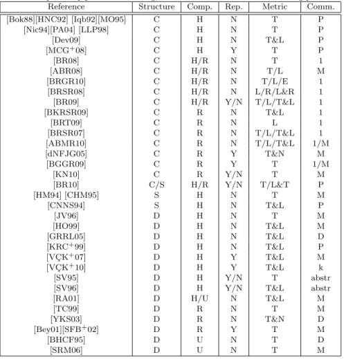
An extensive set of papers dealing with pipelined scheduling is summed up in Table I. Each paper is listed with its characteristics. Since there are too many characteristics to present, we focus on the main ones: structure of the precedence constraints, type of computation, replication, performance metric, and communica-tion model. The table is sorted according to the characteristics, so that searching for papers close to a given problem is made easier. Different papers with the same characteristics are merged into a single line.
The structure of the precedence constraints (the Structure column) can be a single chain (C), a structured graph such as a tree or series-parallel graph (S) or an arbitrary DAG (D). Processing units have computation capabilities (the Comp. column) that can be homogeneous (H), heterogeneous related (R) or heterogeneous unrelated (U). Replication of tasks (the Rep. column) can be authorized (Y) or not (N). The performance metric to compare the schedules (the Metric column) can be the throughput (T), the latency (L), the reliability (R), the energy consumption (E) or the number of processors used (N). The multi-objective problems are de-noted with an & so that T&L denotes the bi-objective problem of optimizing both throughput and latency. Finally, the communication model (the Comm. column) can follow the model with only precedence constraints and zero communication weights (P), the one-port model (1), the multi-port model (M), the k-port model (k), the delay model (D) or can be abstracted in the scheduling problem (abstr). When a paper deals with several scheduling models, the variations are denoted with a slash (/). For instance, paper [BRSR08] deals with scheduling a chain (C) on either homogeneous or heterogeneous related processors (H/R) without using replication (N) to optimize latency, reliability, or both of them (L/R/L&R) under the one-port model (1).
4. FORMULATING THE SCHEDULING PROBLEM
The goal of this section is to build a mathematical formulation of the scheduling problem from a given application. As explained below, it is a common practice to consider a more restrictive formulation than strictly necessary, in order to focus on more structured schedules that are likely to perform well.
Table I. Papers on pipelined scheduling, with characteristics of the scheduling problems.
Reference Structure Comp. Rep. Metric Comm.
[Bok88][HNC92] [Iqb92][MO95] C H N T P [Nic94][PA04] [LLP98] C H N T P [Dev09] C H N T&L P [MCG+08] C H Y T P [BR08] C H/R N T 1 [ABR08] C H/R N T/L M [BRGR10] C H/R N T/L/E 1 [BRSR08] C H/R N L/R/L&R 1 [BR09] C H/R Y/N T/L/T&L 1 [BKRSR09] C R N T&L 1 [BRT09] C R N L 1 [BRSR07] C R N T/L/T&L 1 [ABMR10] C R N T/L/T&L 1/M [dNFJG05] C R Y T&N M [BGGR09] C R Y T 1/M [KN10] C R Y/N T M [BR10] C/S H/R Y/N T/L&T P [HM94] [CHM95] S H N T M [CNNS94] S H N T&L P [JV96] D H N T M [HO99] D H N T&L M [GRRL05] D H N T&L D [KRC+99] D H N T&L P [VC¸ K+07] D H Y T&L M [VC¸ K+10] D H Y T&L k [SV95] D H Y/N T abstr
[SV96] D H Y/N T&L abstr
[RA01] D H/U N T&L M
[TC99] D R N T M
[YKS03] D R N T&N D
[Bey01][SFB+02] D R Y T M
[BHCF95] D U N T D
[SRM06] D U N T M
illustrate the main techniques in Section 4.2. Finally we conclude in Section 4.3 by highlighting the known frontier between polynomial and NP-complete problems.
4.1 Compacting the Problem
One way to schedule a pipelined application is to explicitly schedule all the tasks of all the data sets, which amounts to completely unrolling the execution graph and assigning a start-up time and a processor to each task. In order to ensure that all dependencies and resource constraints are fulfilled, one must check that all predecessor relations are satisfied by the schedule, and that every processor does not execute more than one task at a given time. To do so, it may be necessary to associate a start-up time to each communication, and a fraction of the band-width used (multi-port model). However, the number of tasks to schedule could be extremely large, making this approach highly impractical.
To avoid this problem, a solution is to construct a more compact schedule, which hopefully has some useful properties. The overall schedule should be easily deduced
from the compact schedule in an incremental way. Checking whether the overall schedule is valid or not, and computing the performance index (e.g., throughput, latency) should be easy operations. To make an analogy with compilation, this amounts to transitioning from DAG scheduling to loop nest scheduling. In the latter framework, one considers a loop nest, i.e., a collection of several nested loops that enclose a sequence of scalar statements. Each statement is executed many times, for each value of the surrounding loop counters. Compiler techniques such as Lamport hyperplane vectors, or space-time unimodular transformations [Wol89; DRV00; KA02] can efficiently expose the parallelism within the loop nest, by provid-ing a linear or affine closed-form expression of schedulprovid-ing dates for each statement instance within each loop iteration. On the contrary, a DAG schedule would com-pletely unroll all loops and provide an exhaustive list of scheduling dates for each statement instance.
The most common types of schedules that can be compacted are cyclic sched-ules. If a schedule has a period P, then all computations and communications are repeated every P time units: two consecutive data sets are processed in exactly the same way, with a shift of P time units. The cyclic schedule is constructed from the elementary schedule, which is the detailed schedule for one single data set. If
task ti is executed on processor j at time si in the elementary schedule, then the
execution of this task ti for data set x will be executed at time si+ (x − 1)P on
the same processor j in the cyclic schedule. The elementary schedule is a compact representation of the global cyclic schedule, while it is straightforward to derive the actual start-up time of each task instance, for each data set, at runtime. The re-lation between cyclic and elementary schedule will be exemplified in Sections 4.2.1 and 4.2.2.
With cyclic schedules, one data set starts its execution every P time units. Thus, the system has a throughput T = 1/P. However, the latency L of the application is harder to compute; in the general case, one must follow the entire processing of a given data set (but all data sets have the same latency, which helps simplify the computation). The latency L is the length of the elementary schedule.
Checking the validity of a cyclic schedule is easier than that of an arbitrary schedule. Intuitively, it is sufficient to check the data sets released in the last L units of time, in order to make sure that a processor does not execute two tasks at the same time, and that a communication link is not used twice. Technically, we can build an operation list [ABMR10] whose size is proportional to the original application precedence task graph, and does not depend upon the number of data sets that are processed.
A natural extension of cyclic schedules are periodic schedules, which repeat their operation every K data sets [LKdPC10]. When K = 1, we retrieve cyclic schedules, but larger values of K are useful to gain performance, in particular through the use of replicated parallelism. We give an example in which the throughput increases when periodic schedules are allowed. Suppose that we want to execute a single task of weight 1, and that the platform consists of three different-speed processors P1, P2
and P3with speeds 1/3, 1/5 and 1/8, respectively. For a cyclic schedule, we need to
specify on which processor the task is executed, and the optimal solution is to use the fastest processor, hence leading to a throughput T = 1/3. However, with the
use of replication, within 120 time units, P1can process 40 data sets, P2can process
24 data sets, and P3can process 15 data sets, resulting in a periodic schedule with
K = 40+24+15 = 79, and a throughput T = 79/120, about twice that of the cyclic schedule. Of course it is easy to generalize the example to derive an arbitrarily bad throughput ratio between cyclic and periodic schedules. Note however that the gain in throughput comes with a price: because of the use of replication, it may become very difficult to compute the throughput. This is because the pace of operation for the entire system is no longer dictated by a single critical resource, but instead by a cycle of dependent operations that involves several computation units and communication links (refer to [BGGR09] for details). Periodic schedules are represented in a compact way by a schedule that specifies the execution of K data sets similarly to the elementary schedule of a cyclic schedule.
Other common compact schedules consist in giving only the fraction of the time
each processor spends executing each task [BLMR04; VC¸ K+10]. Such
represen-tations are more convenient when using linear programming tools. However, re-constructing the actual schedule involves advanced concepts from graph theory, and may be difficult to use in practice (although it can be done in polynomial time) [BLMR04].
4.2 Examples
The goal of this section is to provide examples to help the reader understand how to build a scheduling problem from the workflow model, system model and perfor-mance model. We also discuss how the problem varies when basic assumptions are modified.
4.2.1 Chain on Identical Processors with Interval Mapping. We consider the
problem of scheduling a linear chain of n monolithic tasks onto m identical proces-sors (with unit speed), linked by an infinitely fast network. For 1 ≤ i ≤ n, task ti
has a weight pi, and hence a processing time pi on any processor. Fig. 5 presents
an instance of this scheduling problem with four tasks of weights p1 = 1, p2 = 2,
p3= 4, and p4= 3.
When scheduling chains of tasks, several mapping rules can be enforced: —The one-to-one mapping rule ensures that each task is mapped to a different
processor. This rule may be useful to deal with tasks having a high memory requirement, but all inter-task communications must then be paid.
—Another classical rule is the interval mapping rule, which ensures that each pro-cessor executes a set of consecutive tasks. Formally, if a propro-cessor executes tasks tibegin and tiend, then all tasks ti, with ibegin ≤ i ≤ iend, are executed on the same processor. This rule, which provides an extension of one-to-one mappings, is often used to reduce the communication overhead of the schedule.
—Finally, the general mapping rule does not enforce any constraint, and thus any schedule is allowed. Note that for a homogeneous platform with communication costs, [ABR08] showed for the throughput objective that the optimal interval mapping is a 2-approximation of the optimal general mapping.
In this section, we consider interval mappings. Therefore, a solution to the
in-1 2 4 3
t1 t2 t3 t4
Fig. 5. An instance of the chain scheduling problem.
0 1 3 7 10 time
processor
2
1 t1 t2 t3
t4
Fig. 6. The solution of optimal throughput to the instance of Fig. 5 using an interval mapping on two processors.
tervals {I1, . . . , Im}, where Ij (1 ≤ j ≤ m) is a set of consecutive tasks. Note that
one could want to have fewer intervals than processors, leaving some processor(s) completely idle, but here we assume that all the processors are used to make the notation simpler. The length of an interval is defined as the sum of the processing
time of its tasks: Lj =Pi∈Ijpi, for 1 ≤ j ≤ m. Processors are identical (with unit
speed), so that all mappings of intervals onto processors are identical too.
In this case, the intervals form a compact representation of the schedule. The
elementary schedule represents the execution of a single data set: task ti starts
its execution at time si =Pi′<ipi′ on the processor in charge of its interval. An
overall schedule of period P = max1≤j≤mLj can now be constructed: task ti is
executed at time si+ (x − 1)P on the x-th data set. A solution of the instance of
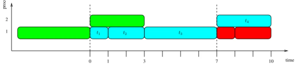
Fig. 5 on two processors that use the intervals {t1, t2, t3} and {t4} is depicted in Fig. 6, where the boxes represent tasks and data sets are identified by colors. The schedule is focused on the cyan data set (the labeled tasks), which follows the green one (partially depicted) and precedes the red one (partially depicted). Each task is periodically scheduled every 7 time units (a period is depicted with dotted lines). Processor 2 is idle during 4 time units within each period.
One can check that such a schedule is valid: the precedence constraints are respected, two tasks are never scheduled on the same processor at the same time
(the processor in charge of interval Ij executes tasks for one single data set during
Lj time units, and the next data set arrives after maxj′Lj′ time units), and the
monolithic constraint is also fulfilled, since all the instances of a task are scheduled on a unique processor.
To conclude, the throughput of the schedule is T = P1 = max 1
1≤j≤mLj, and its
latency is L =P1≤i≤npi. Note that given an interval mapping, T is the optimal
throughput since the processor for which Lj = maxj′Lj′ will never be idle, and it
is the one that defines the period. Note also that the latency is optimal over all
schedules, sinceP1≤i≤npi is a lower bound on the latency.
1 2 processor 0 1 2 3 4 5 7 11 15 17 20 time t2 t1 t3 t4
Fig. 7. The solution of optimal throughput to the instance of Fig. 5 using a general mapping on two processors. processor 2 1 0 1 2 3 4 5 6 10 13 15 20 time t1 t4 t3 t2
Fig. 8. A solution of the same throughput with Fig. 7, but with a better latency. graph, no replication, interval mapping), the problem of optimizing the throughput is reduced to the classical chains-on-chains partitioning problem [PA04], and it can be solved in polynomial time, using for instance a dynamic programming algorithm.
4.2.2 Chain on Identical Processors with General Mapping. This problem is a
slight variation of the previous one: solutions are no longer restricted to interval mapping schedules, but any mapping may be used. By suppressing the interval mapping constraint, we can usually obtain a better throughput, but the scheduling problem and schedule reconstruction become harder, as we illustrate in the following example.
The solution of a general mapping can be expressed as a partition of the task set {t1, . . . , tn} into m sets {A1, . . . , Am}, but these sets are not enforced to be
intervals anymore. The optimal period is then P = max1≤j≤mPi∈Ajpi.
We present a generic way to reconstruct from the mapping a cyclic schedule that preserves the throughput. A core schedule is constructed by scheduling all the tasks according to the allocation without leaving any idle time and, therefore, reaching
the optimal period. Task ti in set Aj is scheduled in the core schedule at time
si =Pi′<i,i′∈A
jpi′. A solution of the instance presented in Fig. 5 is depicted in
Fig. 7 between the dotted lines (time units 0 to 5); it schedules tasks t1 and t3 on
processor 1, and tasks t2 and t4on processor 2.
The notion of core schedule is different than the notion of elementary schedule. Informally, the elementary schedule describes the execution of a single data set while the tasks in the core schedule may process different data sets.
The cyclic schedule is built so that each task takes its predecessor from the previous period: inside a period, each task is processing a different data set. We can now follow the execution of the x-th data set: it starts being executed for task ti
at time si+ (i + x − 1)P, as illustrated for the white data set (x = 0) in Fig. 7.
This technique produces schedules with a large latency, between (n − 1)P and nP. In the example, the latency is 20, exactly 4 times the period. In Fig. 7, the core
schedule is given between the dotted lines (from time step 0 to 5). The elementary schedule is given by restricting the figure to the white data set (i.e., removing all other data sets).
The strict rule of splitting the execution in n periods ensures that no precedence
constraint is violated. However, if the precedence constraint between task ti and
task ti+1 is respected in the core schedule, then it is possible to schedule both of
them in a single time period. Consider the schedule depicted in Fig. 8. It uses the
same allocation as the one in Fig. 7, but tasks t2 and t4 have been swapped in the
core schedule. Thus, tasks t1 and t2 can be scheduled in the same period, leading
to a latency of 13 instead of 20.
Note that the problem of finding the best general mapping for the throughput maximization problem is NP-complete: it is equivalent to the 2-PARTITION prob-lem [GJ79] (consider an instance with two processors).
4.2.3 Chain with a Fixed Processor Allocation. In the previous examples, we
have given hints of techniques to build the best core schedule, given a mapping and a processor allocation, in simple cases with no communication costs. In those examples, we were able to schedule tasks in order to reach the optimal throughput and/or latency.
Given a mapping and a processor allocation, obtaining a schedule that reaches the optimal latency can be done by greedily scheduling the tasks in the order of the chain. However, this may come at the price of a degradation of the throughput, since idle times may appear in the schedule. We can ensure that there will be no conflicts if the period equals the latency (only one data set in the pipeline at any time step).
If we are interested in minimizing the period, the presence of communications makes the problem much more difficult. In the model without computation and communication overlap, it is actually NP-hard to decide the order of communica-tions (i.e., deciding the start time of each communication in the core schedule) in order to obtain the minimum period (see [ABMR10] for details). If computation and communication can be overlapped, the processor works simultaneously on var-ious data sets, and we are able to build a conflict free schedule. When a bi-criteria objective function is considered, more difficulties arise, as the ordering of commu-nications also becomes vital to obtain a good trade-off between latency and period minimization.
4.2.4 Scheduling Moldable Tasks with Series-Parallel Precedence. Chains are
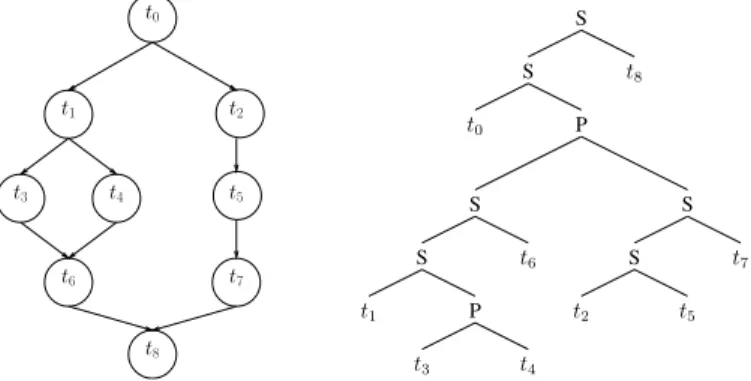
not the only kind of precedence constraints that are structured enough to help derive interesting results. For instance, series-parallel graphs [VTL82] are defined by composition. Given two series-parallel graphs, a series composition merges the sink of one graph with the root (or source) of the other one; a parallel composition merges the sinks of both graphs and the roots of both graphs. No other edges are added or removed. The basic series-parallel graph is composed of two vertices and one edge. Fig. 9 gives an example of a series-parallel graph. The chain of
length three (given as t2, t5 and t7 in Fig. 9) is obtained by composing in series
the chain of length two with itself. The diamond graph (given as t1, t3, t4 and t6
t0 t4 t2 t1 t3 t8 t7 t6 t5 S S P S S P S S t3 t4 t2 t1 t0 t8 t6 t7 t5
Fig. 9. A series-parallel graph, and its binary decomposition tree.
In parallel computing, series-parallel workflow graphs appear when using nested
parallelism [BHS+94; BS05].
[CNNS94] considers the scheduling of series-parallel pipelined precedence task graphs, composed of moldable tasks. A given processor executes a single task and communications inside the moldable task are assumed to be included in the parallel processing times. There is no communication required between the tasks, just a precedence constraint. Provided a processor allocation, one can build an elementary schedule by scheduling the tasks as soon as possible. Since a processor is only involved in the computation of a single task, this elementary schedule reaches the optimal latency (for the processor allocation). Moreover, the elementary schedule can be executed with a period equal to the length of the longest task, leading to a cyclic schedule of optimal throughput (for the processor allocation).
Since the application task graph is a series-parallel graph, the latency and through-put of a solution can be expressed according to its Binary Decomposition Tree (BDT) [VTL82]. Each leaf of the BDT is a vertex of the graph and each internal node is either a series node S(l, r) or a parallel node P (l, r). A series node S(l, r) indicates that the subtree l is a predecessor of the subtree r. A parallel node P (l, r) indicates that both subtrees l and r are independent. A Binary Decomposition Tree is depicted in Fig. 9.
In the BDT form, the throughput of a node is the minimum of the throughputs of the children of the node: T (S(l, r)) = T (P (l, r)) = min(T (l), T (r)). The expression of the latency depends on the type of the considered node. If the node is a parallel node, then the latency is the maximum of the latencies of its children: L(P (l, r)) = max(L(l), L(r)). If it is a series node, the latency is the sum of the latencies of its children: L(S(l, r)) = L(l) + L(r).
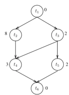
4.2.5 Arbitrary DAGs on Homogeneous Processors. Many applications cannot
be represented by a structured graph such as a chain or a series-parallel graph. Arbitrary DAGs are more general but at the same time they are more difficult to schedule efficiently. Fig. 10 presents a sample arbitrary DAG.
Scheduling arbitrary DAGs poses problems that are similar to those encountered when scheduling chains. Consider first the case of one-to-one mappings, in which each task is allocated to a different processor. A cyclic schedule is easily built by
0 8 2 3 2 0 t1 t2 t3 t6 t5 t4
Fig. 10. An arbitrary DAG (the task weight is the label next to the task).
processor 4 3 2 1 0 1 2 3 4 5 6 7 8 9 10 11 time t3 t5 t2 t4
Fig. 11. One-to-one mapping of the instance of Fig. 10 with L = 11 and T =1
8. Tasks t1and t6 have computation time 0, therefore they are omitted.
scheduling all tasks as soon as possible. Task i is scheduled in the cyclic schedule on processor i at time si = maxi′∈pred(i)si′ + pi′. This schedule can be executed
periodically every P = maxipi with throughput T = max1ipi. The latency is the
longest path in the graph, i.e., L = max si+ pi. A schedule built in such a way
does not schedule two tasks on the same processor at the same time; indeed, each task is executed during each period on its own processor, and its processing time is smaller or equal to the period. Under the one-to-one mapping constraint, this schedule is optimal for both objective functions. The solution for the graph of
Fig. 10 is presented in Fig. 11, with a latency L = 11 and a throughput T = 1
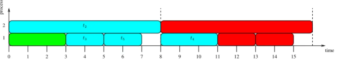
8. When there is no constraint enforced on the mapping rule, problems similar to those of general mappings for linear chains appear (see Section 4.2.2): we cannot easily derive an efficient cyclic schedule from the processor allocation. Establishing a cyclic schedule that reaches the optimal throughput given a processor allocation is easy without communication cost, but it can lead to a large latency. Similarly to the case of chains, a core schedule is obtained by scheduling all the tasks consec-utively without taking care of the dependencies. This way, we obtain the optimal period (for this allocation) equal to the load of the most loaded processor. The cyclic schedule is built so that each task takes its data from the execution of its predecessors in the last period. Therefore, executing a data set takes as many pe-riods as the depth of the precedence task graph. On the instance of Fig. 10, the
optimal throughput on two processors is obtained by scheduling t2 alone on a
0 1 2 3 4 5 6 7 8 9 10 11 time 1 2 processor 12 13 14 15 t3 t2 t4 t5
Fig. 12. A general mapping solution of the instance of Fig. 10 with L = 15 and T =1
8. Tasks t1 and t6 have computation time 0, therefore they are omitted.
0 1 2 3 4 5 6 7 8 9 10 11 time 1 2 processor 12 13 14 15 t2 t5 t3 t4
Fig. 13. A general mapping solution of the instance of Fig. 10 with L = 11 and T =18. Tasks t1 and t6 have computation time 0, therefore they are omitted.
this generic technique, leading to a latency L = 15. Note that t5could be scheduled
in the same period as t3 and in general this optimization can be done by a greedy
algorithm. However, it does not guarantee to obtain the schedule with the optimal latency, which is presented in Fig. 13 and has a latency L = 11. Indeed, contrarily to linear pipelines, given a processor allocation, obtaining the cyclic schedule that minimizes the latency is NP-hard [RSBJ95].
The notion of interval mapping cannot be directly applied on a complex DAG. However, we believe that the interest of interval mapping schedules of chains can be transposed to convex clustered schedules on DAGs. In a convex clustered sched-ule, if two tasks are executed on one processor, then all the tasks on all the paths between these two tasks are scheduled on the same processor [LT02]. Convex clus-tered schedules are also called processor ordered schedules, because the graph of the inter-processor communications induced by such schedules is acyclic [GMS04]. The execution of the tasks of a given processor can be serialized and executed with-out any idle time (provided their execution starts after all the data have arrived). This leads to a reconstruction technique similar to the one applied on chains of tasks following the interval mapping rule. Two processors that are independent in the inter-processor communication graph can execute their tasks on a given data set during the same period in any order, without violation of the precedence con-straints. Such a construction leads to the optimal throughput for a given convex clustered mapping of the tasks to the processors, and to a latency L ≤ xP ≤ mP, where x is the length of the longest chain in the graph of communications between processors.
Algorithms to generate convex clustered schedules based on recursive decom-position have been proposed for classical DAG scheduling problems [PST05]. In pipelined scheduling, heuristic algorithms based on stages often generate convex clustered schedule such as [BHCF95; GRRL05]. However the theoretical properties of such schedules have never been studied for pipelined workflows.
0 1 2 3 4 5 6 7 8 9 10 11 1 2 12 13 14 processor 3 time t3 t2 t5 t3 t5 t4 t2 t4
Fig. 14. A general mapping solution of the instance of Fig. 10 with L = 14 and T = 1
7 when task t2is replicable. Tasks t1and t6have computation time 0, therefore they are omitted.
4.2.6 Scheduling Arbitrary DAGs on Homogeneous Processors with Replication.
A task is replicable if it does not contain an internal state. It means that the same task can be executed at the same time on different data sets. Replication allows one to increase the throughput of the application. (We point out that this is different from duplication, which consists in executing the same task on the same data set on multiple different processors. Redundantly executing some operations aims at either reducing communication bottlenecks, or increasing reliability.) On the instance presented in Fig. 10, only two processors can be useful: the dependencies prevent any three tasks from being executed simultaneously, so a third processor would improve neither the throughput nor the latency for monolithic tasks. However, if
task t2is replicable, the third processor could be used to replicate the computation
of this task, therefore leading to the schedule depicted in Fig. 14.
Replicating t2 leads to a periodic schedule that executes two data sets every 14
time units (K = 2). Its throughput is therefore T = 142 = 17, which is better than
without replication. The latency is the maximum time a data set spends in the system. Without replication, all the data sets spend the same time in the system. With replication, this statement no longer holds. In the example, the cyan data set spends 11 time units in the system whereas the green one spends 14 time units.
The latency of the schedule is therefore L = 14. If task t4 was replicable as well,
two copies could be executed in parallel, improving the throughput to T = 112 and
the latency to L = 11. A fourth processor could be used to pipeline the execution
of t4 and reach a period of P = 8 and, hence, a throughput of T = 1
4.
A schedule with replication is no longer cyclic but instead is periodic, with the definitions of Section 4.1. Such a schedule can be seen as a pipelined execution of an unrolled version of the graph. The overall schedule should be specified by giving a periodic schedule of length ℓ (the time between the start of the first task of the first data set of the period and the completion of the last task of the last data set of the period), detailing how to execute K consecutive data sets, and providing its period P. Verifying that the schedule is valid is done in the same way as for classical elementary schedules: one needs to expand all the periods that have a task running during the schedule, that is to say the tasks that start during the elementary schedule and within the ℓ time units before. Such a schedule has a
throughput of T =K
P, and its latency should be computed as the maximum latency
of the data sets in the elementary schedule.
all the m processors. Each processor executes sequentially exactly one copy of the
application. This leads to a schedule of latency and period P = L =Pipi, and a
throughput of T = Pm
ipi .
When using replication, it is possible that data set i is processed before its pre-decessor i − 1. This behavior mainly appears when processors are heterogeneous. The semantic of the application might not allow data sets to be processed in such an out-of-order fashion. For instance, if a task is responsible for compressing its input, providing the data sets out-of-order will change the output of the program. One can then either impose a delay, or use some other constraints, as for instance the dealable stage constraint [Col04].
4.2.7 Model Variations. In most cases, heterogeneity does not drastically change
the scheduling model. However, the compact schedule description must then con-tain the processor allocation, i.e., it must specify which task is executed on which processor. Otherwise the formulations stay similar.
A technique to reduce latency is to consider duplication [AK98; VC¸ K+10].
Du-plicating a task consists in executing the same task more than once on different processors for every data set. Each task receives its data from one of the duplicates of each of its predecessors. Hence, this allows more flexibility for dealing with data dependency. The idea is to reduce the communication overheads at the expense of increasing the computation load. Another goal is to increase the reliability of the system: whenever the execution of one duplicate would fail, that of another dupli-cate could still be successful. The major difference of duplication as compared to replication is the following: with duplication, a single data set is executed in each period, whereas with replication, several data sets can be executed in each period. Communication models affect the schedule formulation. The easiest communi-cation model is the one-port model where a machine communicates with a single other machine at a time. Therefore, in the schedule, each machine is represented by two processors, one for the computations and one for the communications. A valid schedule needs to “execute” a communication task at the same time on the communication processor of both machines involved in the data transfer. A com-mon variation on the one-port model is to forbid communication and computation overlap. This model is used in [HO99]. In this case, there is no need for a communi-cation processor; the communicommuni-cation tasks have to be scheduled on the computation processor [BRSR07].
To deal with more than one communication at a time, a realistic model would be to split the bandwidth equally among the communications. However such models are more complicated to analyze, and are therefore not used in practice. Two ways of overcoming the problem exist. The first one is to consider the k-port model where each machine has a bandwidth B divided equally into k channels. The scheduling problem amounts to using k communication processors per machine. This model has been used in [VC¸ K+10].
When only the throughput matters (and not the latency), it is enough to ensure that no network link is overloaded. One can reconstruct a periodic schedule ex-plicitly, by using the model detailed previously, considering each network link as a processor. This approach has been used in [TC99].
4.3 Complexity
The goal of this section is to provide reference pointers for the complexity of the pipelined scheduling problem. Lots of works are dedicated to highlighting the fron-tier between polynomial and NP-hard optimization problems in pipelined schedul-ing.
The complexity of classical scheduling problems have been studied in [Bru07]. One of the main contributions was to determine some constraint changes that al-ways make the problem harder. Some similar results are valid on pipelined schedul-ing. For instance, heterogeneous versions of problems are always harder than their homogeneous counterpart, since homogeneous cases can be easily represented as heterogeneous problem instances but not vice versa. A problem with an arbitrary task graph or architecture graph is always harder than the structured counter-part, and in general considering a superset of graphs makes problems harder. Also, removing communications makes the problem easier.
As seen in the previous examples, throughput optimization is always NP-hard for general mappings, but polynomial instances can be found for interval mappings. The communication model plays a key role in complexity. The optimization of latency is usually equivalent to the optimization of the makespan in classical DAG scheduling [KA99b].
The complexity of multi-objective problem instances relates to three different types of questions. First, the decision problems of multi-objective problems are di-rectly related to those for mono-objective problems. A threshold value is given for all the objectives, and the problem is to decide whether a solution exists, that matches all these thresholds. Multi-objective decision problems are obviously harder than their mono-objective counter part. Second, the counting problem con-sists in computing how many Pareto-optimal solutions a multi-objective problem has; a Pareto-optimal solution is such that no other solution is strictly better than it. Finally, the enumeration problem consists in enumerating all the Pareto-optimal solution of an instance. The enumeration problem is obviously harder than the de-cision problem and the counting problem, since it is possible to count the number of solutions with an enumeration algorithm, and to decide whether given thresholds are feasible. A complete discussion of these problems can be found in [TB07].
The complexity class of enumeration problems expresses the complexity of the problem as a function of both the size of the input of the problem and the number of Pareto-optimal solutions leading to classes EP (Enumeration Polynomial) and ENP (for Enumeration Non-deterministic Polynomial) [TBE07]. Therefore, the decision version of a multi-objective problem might be NP-complete, but since it has an exponential number of Pareto optimal solution, its enumeration version is in EP (the
problem 1 ||PCA
i ; P
CB
i of [AMPP04] is one of the many examples that exhibit
this property). Therefore, the approaches based on exhaustive enumeration can take a long time. However, [PY00] shows that most multi-objective problems admit an approximate set of Pareto optimal solutions whose cardinality is polynomial in the size of the instance (but it is exponential in the number of objectives and in the quality of the approximation). It was also shown in [PY00] that an approximation algorithm for the decision problem can be used to derive an approximation of the Pareto set in polynomial time. These results motivate the investigation of