Coordinated tracking and interception of an acoustic target using autonomous surface vehicles

Coordinated Tracking and Interception of an Acoustic Target

Using Autonomous Surface Vehicles

by

Lieutenant Ryan Lee Conway, United States Navy

Submitted to the Joint Program in Applied Ocean Science & Engineering in partial fulfillment of the requirements for the degree of

Master of Science in Mechanical Engineering MASSACHUSE

at theOF TECH

at the

MASSACHUSETTS INSTITUTE OF TECHNOLOGY

and the

SEP

1

WOODS HOLE OCEANOGRAPHIC INSTITUTION

-September 2019

LIBRA

@2019

ARCHI

All rights reserved.

The author hereby grants to MIT and WHOI permission to reproduce and to distribute publicly paper and electronic copies of this thesis document in whole or i

part in any medium now known or hereafter created.

Signature redacted

9

2019

~RIES

VES

A uth or ...

Joint Program in Applied Ocen Science & Engineering

Massachusetts Institute of Technology

&Woods Hole Oceanographic Institution

August 9, 2019

Signature redacted

Certified by...

Accepted by...

...

.... ...

...

Erin Fischell

Assistant Scientist

Woos Hpl,

anographic Institution

Signature redactedThesis

Supervisor

Henrik Schmidt

L

sfesor of Mieaiand Ocean Engineering

rs

usetts Institute of Technology

Signature redacted

_....

_...

Nicolas Hadjiconstantinou

Chair, Mechanical Engi eering Committee for Graduate Students

Massachusetts Institute of Technology

...

Signatureredacted

David Ralston

Chair, Joint Committee for Applied Ocean Science & Engineering

Woods Hole Oceanographic Institution

Coordinated Tracking and Interception of an Acoustic Target Using

Autonomous Surface Vehicles

by

Lieutenant Ryan Lee Conway, United States Navy

Submitted to the Joint Program in Applied Ocean Science & Engineering Massachusetts Institute of Technology

&Woods Hole Oceanographic Institution on August 9, 2019, in partial fulfillment of the

requirements for the degree of

Master of Science in Mechanical Engineering

Abstract

In today's highly advanced society, more industries are beginning to turn to autonomous ve-hicles to reduce costs and improve safety. One industry in particular is the defense industry. By using unmanned and autonomous vehicles, the military and intelligence communities are able to complete missions without putting personnel in harm's way. A particularly impor-tant area of research is in the use of marine vehicles to autonomously and adaptively track a target of interest in situ by passive sonar only. Environmental factors play a large role in how sound propagates in the ocean, and so the vehicle must be able to adapt based on its surrounding environment to optimize acoustic track on a contact. This thesis examines the use of autonomous surface vehicles (ASVs) to not only autonomously detect and localize a contact of interest, but also to conduct follow-on long-term tracking and interception of the target, by using anticipated environmental conditions to motivate its decisions regard-ing optimum trackregard-ing range and speed. This thesis contributes a simulated and theoretical approach to using an ASV to maximize signal-to-noise ratio (SNR) while tracking a contact autonomously. Additionally, this thesis demonstrates a theoretical approach to using infor-mation from a collaborating autonomous vehicle to assist in autonomously intercepting a target.

Thesis Supervisor: Erin Fischell Title: Assistant Scientist

Acknowledgments

The research completed in this thesis was funded by the U.S. Navy's Civilian Institution Program with MIT/WHOI Joint Program. Thank you to the Navy and the Submarine Community for providing me with this amazing opportunity to study at these two premiere institutions.

Thank you to my thesis advisor, Dr. Erin Fischell, for all of your support on my research and coursework. Your never-ending support and guidance amidst your busy schedule enabled me to successfully complete my research on schedule. I appreciate all of the valuable feedback you provided to me along the way and wish you and your family all the best.

Thank you to Kevin Manganini for your support with hardware development, and your expert knowledge of Jetyak operations. Without your assistance I would not have been able to collect all of the necessary acoustic data.

I would also like to thank Professor Henrik Schmidt and Professor Arthur Baggeroer for their tireless support of all of the Navy MIT/WHOI Joint Program students. The support you have provided to the Navy students over the years has ensured the continued success of the partnership between the Navy and Joint Program. Because of your mentorship, I am confident that future Navy students will continue to succeed in the Joint Program. Dr. Schmidt, I wish you the best of luck as you transition into retirement.

Additionally, I would like to thank Dr. Michael Benjamin and Caileigh Fitzgerald. You patiently put up with me, and answered countless questions of mine throughout the Marine Vehicle Autonomy course. Your assistance helped me to develop the skills necessary to successfully complete my research.

Next, I would like to thank my classmates, especially Andrew Cole and Andrew Johnson. Thank you for all of your support, professional and academic guidance, and friendship. I look forward to following your Navy careers, and seeing the amazing things you do for the Submarine Force and Surface Fleet.

Finally, I would like to thank my wife, Eilish, and my two daughters, Catriona and Clare, for all of your love and support over the past two years. I will forever be thankful for all of the sacrifices that you have made to allow me to pursue this opportunity. Eilish, I am in constant awe of how well you have handled the stress of having both of us in graduate school, while also providing for our girls on the countless days and nights that I was studying late.

You are the most talented person I have ever met and I look forward to our next adventure together.

Contents

2.1 Acoustic Propagation in the Ocean . . . . 2.2 Acoustic Rays . . . ..

2.2.1 Ray Tracing . . . .

2.2.2 Eigenrays and Transmission Loss . . . .

3 Source Detection and Tracking

3.1 Acoustic Arrays and Beamforming . . . . 3.1.1 Uniform Line Arrays . . . . 3.2 Tracking . . . . 3.2.1 Classical Kalman Filter Overview . . . . 3.2.2 Extended Kalman Filter . . . .

4 Experimental Methods

4.1 Jetyak Autonomous Surface Vehicle . . . . 4.2 Acoustic Data Collection . . . . 4.2.1 JetYak Self-Noise vs. Speed Test . . . . 4.2.2 Source Detection and SNR Experiment . 4.3 MOOS-IvP Simulations . . . . 15 15 16 17 17 19 19 20 21 23 25 26 27 31 32 33 37 38 39 39 40 42 . . . . . - . . . .

4.3.1 MOOSApps ... ... ... 43

4.3.2 M OOSBehaviors . . . .. 44

4.3.3 Shallow Water Summer Profile... . . . . . . . 44

5 Results 47 5.1 Jetyak Self-Noise vs. Speed Test Results... . . . .. 47

5.1.1 Jetyak 1 . . . . . . . 47

5.1.2 Jetyak 2 . . . . . . . . . . 48

5.2 Field R esults . . . 49

5.2.1 Test 1 - Stationary source on the dock with a single vehicle . . . 50

5.2.2 Test 2 - Stationary source in the harbor with two vehicles . . . 53

5.3 Shallow Water Summer Profile Simulation Results . . . 56

5.3.1 Tracking Vehicle . . . .. 58

5.3.2 Intercept Vehicle . . . 59

5.3.3 Source Position Error . . . .... . 60

5.4 Conclusion . . . . . . . 61

6 Future Work and Concluding Remarks 63

List of Figures

2-1 Depiction of fluid-fluid interfaces in the ocean [11] . . . . . 20

2-2 Illustration of bracketing rays in depth around a receiver [12]. . . . 23

3-1 Coordinate system used for beamforming 127]. . . . 26

3-2 Uniform Line Array with N-elements and elemental spacing Az [27]. . . . 27

3-3 Visualization of an acoustic array with linear processing [27] . . . .. 28

3-4 Delay-and-sum beamforming process [27] . . . 30

3-5 Illustration of crossed bearings between two moving receivers and one moving target. . . . 31

4-1 Test Site for each Jetyak Self-Noise vs. Speed Test [6]. . . . 38

4-2 One of two Jetyak ASVs used during real-world experiments, collecting acous-tic data to demonstrate the effects of range and speed on the RL of the re-ceived signal emitted from the source. . . . 39

4-3 Flow of information between front seat and back seat computers for au-tonomous decision-making. . . . 40

4-4 HTI-96-MIN hydrophone [10]. . . . 41

4-5 Data flow process from eight element hydrophone array to storage on a Rasp-berry Pi 3 Model B Computer. . . . 41

4-6 Vehicle and Source configurations for the two acoustic experiments performed. (a) Test 1 configuration with vehicle tracks perpendicular to each other and sound source placed at the WHOI pier; (b) Test 2 configuration with vehicles passing fixed sound source in the harbor [6] . . . 42

4-7 Flowchart of MOOSApps that were developed in support of this thesis . . . . 43

4-9 Transmission Loss vs Range plot for a 1 kHz source at a depth of 1 meter

and a receiver at 1 meter . . . . . . . 45

5-1 Spectrogram of acoustic data collected on Jetyak 1 in Woods Hole Harbor, Massachusetts on March 28, 2019 . . . . .. 48

5-2 Raw RL vs. Speed of Jetyak 1 . . . .. 49

5-3 Filtered RL vs. Speed of Jetyak 1. . . . . .. 49

5-4 Linear interpolation of data obtained from Jetyak 1 test experiment, modeling the estimated transmission loss vs speed. . . . 50

5-5 Raw RL vs. Speed of Jetyak 2 . . . . . . . . .. . 51

5-6 Filtered RL vs. Speed of Jetyak 2. . . . 51

5-7 Linear interpolation of data obtained from Jetyak 2 test experiment, modeling the estimated transmission loss vs speed. . . . 52

5-8 RL vs Time plotted alongside Range and Speed vs. Time for Test 1 . . . .52

5-9 Expected vs Actual RL Results for Test 1. . . . 53

5-10 Spectrogram from Jetyak 1, showing the 1 kHz source . . . . . . . 54

5-11 RL vs Time plotted alongside Range and Speed vs. Time for Jetyak 1, Test 2. 54 5-12 RL vs Time plotted alongside Range and Speed vs. Time for Jetyak 2, Test 2. 55 5-13 Expected vs Actual RL Results for Jetyak 1, Test 2. . . . 55

5-14 Expected vs Actual RL Results for Jetyak 2, Test 2 . . . . ... 56

5-15 Example output from beamforming Jetyak 1 acoustic data. . . . 56

5-16 Expected vs. estimated bearing from Jetyak 1 conventional beamforming. . . 57

5-17 Expected vs. estimated bearing from Jetyak 2 conventional beamforming. . . 57

5-18 Plot of the source and the tracking vehicle tracks, as the tracking vehicle repositions to optimize RL. . . . 58

5-19 Simulation results for the tracking vehicle. (a) Tracking vehicle speed vs. time; (b) Filtered SNR of the received signal, assuming a 70 dB ambient background noise; (c) Vehicle range vs. time overlaid on the shallow water summer profile plot of SL - TL, illustrating which range the vehicle chose as the optimal range... . . . .. 59

5-20 Intercept and Source Tracks vs. Time . . . 60

List of Tables

4.1 Summary of acoustic array design specifications . . . ... 39 4.2 Operating characteristics of Lubell LL916C underwater acoustic source . 42 4.3 Initial conditions of shallow water summer simulation . . . .. 46 5.1 Speed vs. SNR results for Jetyak 1. . . . . . . . .50 5.2 RL versus speed results for Jetyak 2 . . . . 53

Chapter 1

Introduction

1.1

Motivation

Operating a manned vessel out at sea requires significant resources. Between the crew salary, maintenance costs, fuel, and technical support, operating costs for a warship or research ves-sel is easily in the millions of dollars per year, and the costs are continuing to rise. In a 2009 study by the National Research Council of the National Academies, it was noted that between 2000 and 2008 the total number of at-sea operating days by the University-National Oceanographic Laboratory System (UNOLS) had dropped by 13%, but the total operating costs increased by 75%, doubling the acerage costs per day [4].

More important than the financial resources required to operate a ship at sea, operating a manned vessel is inherently dangerous. In the summer of 2017 the U.S. Navy had two high profile collisions while operating in areas with high shipping densities

122].

[211.

Due to the rising costs and inherent danger associated with operating manned vessels, several industries, including national defense, are turning to autonomous marine systems, which include autonomous surface vehicles (ASVs) and autonomous underwater vehicles (AUVs). Autonomous vehicles are relatively low-cost, easy to deploy, difficult to detect, and unmanned, so the risks that were previously associated with carrying out a mission

(both financially and personnel-wise) are significantly reduced. As a result of this, use of autonomous vehicles will be a critical component of future naval operations.

One area of interest for these autonomous systems is detection, classification, localiza-tion and tracking (DCLT) using passive acoustics. In the autonomous DCLT mission, an unmanned vessel uses a hydrophone array, data aquisistion system, and signal processing software to provide a remote user with information on nearby vessels and acoustic conditions. Passive autonomous DCLT technology is an area of active research, and with increased size, speed, and autonomy capability of ASVs a critical area of interest is how to best use multiple vehicles in the DCLT mission. Some areas in the autonomy decision space include how to position multiple vehicles for passive tracking of targets, autonomous response to detection, and communication and coordination approaches. This thesis describes research into use of two gasoline-powered ASVs to demonstrate detection, tracking, and interception of a target.

1.2

Background

There are several different methods that researchers and defense personnel employ to local-ize and track a contact in the ocean, such as RADAR, active SONAR, and passive SONAR. While RADAR and active SONAR provide high fidelity solutions to the contact of interest, there are increased counter-detection risks associated with using them (a particular concern for submarines and AUVs). As a result, one of the most commonly used methods to detect, localize and track a contact of interest is passively via a bearings-only approach.

There has been extensive research done in the field of passive acoustic tracking. Most array processing texts, including Van Trees [271, cover the theory and real-world applica-tion of passively tracking a sound source extensively. There are also excellent examples of papers that demonstrate single-vehicle adaptation to improve beamformed SNR and break left-right ambiguity, e.g. [2],[7].

The Maritime Security Laboratory at the Stevens Institute of Technology has also done work in this field, developing an underwater passive acoustic array that has successfully de-tected, classified, and tracked various noise sources, such as divers, surface vessels and AUVs [3],[23]. Another example of progress made in the development of passive acoustic systems is work done by the Ocean Acoustical Services and Instrumentation Systems (OASIS, Inc.), which has demonstrated the feasibility of tracking AUVs with a passive acoustic system

in harsh harbor environments [1]. Additionally, there have been several studies providing information on expected signal to noise ratio and frequency content of different types of surface vessels [17],[30].

One noticeable gap in the current state of research is using passive acoustics as well as ocean modeling to inform an autonomous vehicle's decision on where to track a target of interest from in order to optimize signal-to-noise ratio and most effectively track the contact.

1.3

Contributions

The key contributions of this thesis include:

" SNR modelling to inform autonomy that includes self-noise, array gain, and acoustic propagation of target noise.

" Development and deployment of an array system for Jetyak ASVs

•

" Field experiments to test autonomy.

1.4

Organization

This thesis is organized into six chapters. Chapter 2 discusses acoustic propagation in an ocean environment and the calculation of acoustic rays for use in modeling software. Chapter 3 discusses common techniques to detect and track a sound source or contact of interest. Chapter 4 explains the experimental methods that were used to both simulate a realistic tracking problem, as well as collect real-world acoustic data. Chapter 5 displays the results of simulations and real-world experiments. Finally, conclusions and recommended future work are discussed in Chapter 6.

Chapter 2

Acoustic Propagation

A critical aspect of this thesis is to optimize the signal-to-noise ratio (SNR) of a signal that a receiver collects from a sound pressure wave emitted from a sound source in the water. To successfully do this, the ocean environment and sound sound propagation must be accurately modeled. This chapter presents a mathematical background of how sound propagates through the ocean, and describes the process used to accurately calculate the transmission loss at a particular point in the ocean, which will be used to calculate the received level (RL) and SNR.

2.1

Acoustic Propagation in the Ocean

In the ocean, the surrounding environment is a significant factor in how an acoustic wave propagates and how far it travels before being attenuated below a detectable level. The speed of sound in the ocean is dependent on water density, which is a function of pressure/depth

(z), salinity (S), and temperature (T), as defined in Equation 2.1 13].

c = 1449.2 + 4.6T - 0.055T2 + 0.00029T3 + (1.34 - 0.01T)(S - 35) + 0.016z (2.1)

The water temperature, pressure, and salinity can vary greatly within a water column, and as a result of this, the ocean can be viewed as a layered acoustic waveguide with an infinite number of interfaces stacked together as depicted in Figure 2-1 [12]. Similar to

Figure 2-1: Depiction of fluid-fluid interfaces in the ocean [11].

optical waves, acoustic waves bend according to Snell's law [121:

k1cos 01 = k2 cos 02 = k, cos 0, (2.2)

where k, the acoustic wavenumber, is a function of angular frequency (w) and sound speed

(c) as defined in Equation 2.3, and 0 is the incident angle of the wave at the interface.

k (2.3)

C

2.2

Acoustic Rays

In the previous section, it was noted that acoustic waves observe Snell's Law of refraction. Using this, acousticians have developed different techniques to calculate the expected path that a sound pressure wave takes for a given sound speed profile, as well as the expected pressure amplitude of the propgating sound at a particular point. Some of the most com-monly employed models are either normal mode calculations or ray tracing models, each with their own advantages and disadvantages [121. Ray tracing models tend to be less ac-curate than normal mode models, however take much less processing power and therefore have faster processing times. For the purpose of this thesis, a ray tracing model was used, and will be discussed in greater detail in the following section.

ki

k2

k3 83

2.2.1 Ray Tracing

To calculate the path and amplitude of an acoustic wave along a single ray, we begin with the Helmholtz equation [12]:

P + 2(p = -6(x - xo), (2.4)

where xO is the location of the sound source and x=(x,y,z). To get the ray equations, we assume a solution to the Helmholtz equation in the form of:

p(x) = e ()(2.5)

n=o

After taking the first and second derivatives of Equation 2.5, and solving for V2p, we insert the result back into Equation 2.4 to get the result in terms of two separate equations: a non-linear partial differential equation (PDE) known as the Eikonal equation and an infi-nite series of of linear PDEs known as the transport equation [12].

The Eikonal equation, defined in Equation 2.6 can be solved using many different meth-ods, but is often solved by introducing a family of rays perpendicular to the wavefronts. This method allows us to define the ray trajectory x(s) by the differential equation in Equation 2.7. 1 Vr|2 =(2.6)_c2 (x)(26 dx_dx= cVr (2.7) ds

Next, we differentiate the x,y, and z components of Equation 2.7 with respect to s to obtain: d 1 dx 1

( =- Vc (2.8)

Finally, the ray equations can be written in the form: dr_{-- = c (,} (2.9) ds d z = c((s), (2.10) ds d< 1 oc ds c2 r' d( 1 09C(2.12)

where r(s) and z(s) is the trajectory of the ray in the range-depth plane [12].

Now that the Eikonal equation has been solved, the transport equation must be solved to calculate the pressure amplitude along the ray. The transport equation is defined in Equation 2.13:

V (A'Vr) = 0 (2.13)

By applying Gauss's divergence theorem to Equation 2.13, we are left with:

jA

V0r

where n is an outward pointing normal vector. Next, by grouping a family of rays together, we can define the volume enclosed by the rays as a "ray tube". Since rays are normal to the phase fronts, the ray is the normal vector on the ends of the ray tube, resulting in V -n = 1_C on the ends of the ray tube and

V

we determine that:

J

_8aVO

_C

As the ray tube becomes infinitesimally small, we are left with:

Ao(s)= Ao(0) c(0) J(0), (2.16)

2.2.2

Eigenrays and Transmission Loss

By applying the methods described in Section 2.2.1, we were able to calculate the amplitude of the pressure along a single ray. However, we also often want to know what the pressure field looks like at a particular point. Because multiple rays can pass through a single point (known as eigenrays), and each one contributes to the pressure field based on its intensity and phase at that point, we must find all eigenrays to determine the total amplitude of the pressure field at that point.

To find the eigenrays, we start by tracing a fan of rays, and then identify pairs of rays with adjacent take-off angles that bracket the receiver in depth, as shown in Figure 2-2, and finding the phase delay and amplitude through linear interpolation. As can be seen

r

Source

z

Figure 2-2: Illustration of bracketing rays in depth around areceiver [12].

in Figure 2-2, two rays with adjacent take-off angles that bracket areceiver in depth may have different ray histories (i.e. one may have had asurface orbottom interaction, while the other ray was direct path). Since large errors can result by interpolating the results of two rays with different histories, interpolation is performed in this case.

Once all of the eigenrays have been determined, the total pressure intensity is calculated by summing up the contributions of each eigenray, as shown in Equation 2.18.

N(r,z)

p(C) (r, z) = Epj (,z) (2.18)

Once the intensity has been determined, we can calculate the transmission loss at the par-ticular point as:

TL(s)= -20 log p(S) (2.19)

where po(s = 1) =

Once the transmission loss is calculated, the RL and SNR can be calculated using the passive sonar equation

[25],

Chapter 3

Source Detection and

Tracking

As was discussed in Chapter 2, the transmission loss at any given point in the ocean is heavily dependent on the environment in which the acoustic wave is propagating, and the transmission loss can be estimated through various techniques. Assuming deep water, and a mid-water-column sound source, the basic passive sonar equation can be used to describe the received level of sound based on the source level (SL) and the transmission loss (TL), as well as the background noise level (N) [29]:

RL = SL - TL + N, (3.1)

Additionally, the SNR can be described as:

SNR = RL - N. (3.2)

The SL is the acoustic level of the source referenced 1 meter from the source, TL is the transmission loss the acoustic wave due to the distance the wave travels from the source to the receiver, NL is the background noise level including ownship noise and background noise levels [29], all measured in decibels (dB).

The received sound is detected by a hydrophone or transducer, which measures changes in sound pressure levels. This signal is then converted to an electrical signal, where it is processed to determine direction of arrival or bearing. Once the direction of arrival has been established, this information can be applied to various state estimation algorithms to estimate the position, course, and speed of the source. This chapter presents the

math-ematical basis for the detection and tracking algorithms that were used in this thesis, to autonomously localize and track a sound source in the water.

3.1

Acoustic Arrays and Beamforming

Beamforming is used to determine the bearing from the sound source to the receiver. The array filters the signals in a "space-time field by exploiting their spacial characteristics" [27]. The filtered signals are expressed as a function of wavenumber, where the wavenumber for a plane wave in a locally homogeneous medium is defined as:

sin 0 cos k = -2rsin 0 sin

4(3.3)

cos 0

As shown in Figure 3-1, 0 is the polar angle with respect to the z-axis,

#

The geometry of the array that is chosen affects the performance and operation of it.

Polar Angle

AzlmuthAngle

Figure 3-1: Coordinate system used for beamforming [27].

For example, when a line array is used, only one angular component is resolved, resulting in right/left bearing ambiguities [27]. Additionally, the array length, spacing between the sensors, sampling frequency, and weighting at each sensor output significantly affects the array's performance.

3.1.1 Uniform Line Arrays

In this thesis, a horizontal line array with equally spaced hydrophones was used. This is known as a uniform line array [27], and is pictured in Figure 3-2.

n=N-1 4I I I I I I n=0

*

Figure 3-2: Uniform Line Array with N-elements and elemental spacing Az [27].

The sensor locations are defined

[27]

PXn = Pyn = 0

Pz = (n - N 1)Az, for n = 0, 1,..., N - 1 2

The array elements sample the field, resulting in a vector of signals:

f (t, po) f(t,p)=

f(tPI)

The array output, y(t), is then realized by processing the output of each sensor through an impulse response filter, ha(r), and summing them together

[27],

N-1i

y(t)= Ej h(t - r)f(-r, p)dr (3.7)

n=o

= j hT(t - r)f(r, pn)dr, (3.8)

and visualised in Figure 3-3.

In lieu of Equation 3.8, the array output can be written more succinctly in the transform

f(t,po)

f

~

fMtpN-1 N-1 _ft

Figure 3-3: Visualization of an acoustic array with linear processing

[27]

domain as [27]: Y(w) HT (w)F(w), (3.9) where H(w)= h(t)e-jwtdt, (3.10) and F(w)= f(t, p')e~wtdt. (3.11)

Assuming the acoustic wave from the target of interest propagates as a plane wave, the signal received at each sensor is:

f(t -To)

f

f

f(t

where -r is the time delay in arrival at each sensor and is defined

[27]

7 = ( ,p, sin 6 cos $ + py, sin 0 sin

#

c

In the case of a linear array, as used in this thesis, Equation 3.13 can be reduced to:

rn -Pz' cos 0 (3.14) C

Using Equations 3.11 and 3.12, the nth component of F(w) is [27]:

Fn(w) =

f

(3.16)

where

wr = kT pn. (3.17)

The exponential term of 3.16 can be rewritten in terms of an array manifold vector [27]:

e-jkTpo e-jkTp1

Vk (k)= (3.18)

and therefore,

Fn(w) = F(w)vk(k) (3.19)

As before, the output of each sensor is processed through a filter, hn(T), defined as:

h(-r) = 1o(r + rn) (3.20)

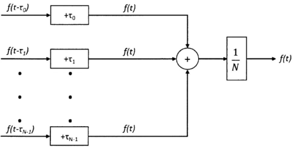
to align all of the signals in time. The signals are then summed together to obtain the output y(t) = f(t), as illustrated in Figure 3-4. This process is known as "delay-and-sum beamforming" or "conventional beamforming" [27]. In the frequency domain this can be

f(t)

f(t-T1)

f(t)1

+r, + -f(t)

f(t-rN-1) f(t)

lt +rN-1

Figure 3-4: Delay-and-sum beamforming process

[271

compactly written as:

H T(w) = I vk H (ks) (3.21)

By combining Equations 3.18 and 3.21, we arrive obtain the frequency-wavenumber response to a plane wave [27]:

(3.22) f(t-ro)

iFILr

Finally, the beam pattern is calculated by evaluating the frequency-wavenumber response versus the steering direction:

B(w : 0, # = Y(w, k)|k= !a(0,4) (3.23)

3.2

Tracking

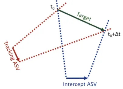
After beamforming a signal, a single receiver will have a relative direction to the source, however range is still unknown; the target of interest can be anywhere down that bearing. By adding a second receiver at a different location, the position and range are able to be determined by calculating the position at which the bearings cross, as illustrated in Figure 3-5.

to *•

Intercept ASV

Figure 3-5: Illustration of crossed bearings between two moving receivers and one moving target.

Assuming perfect data (i.e. not noise corrupted and perfect bearing resolution) a perfect system solution to the source can be obtained after each receiver obtains

just

algorithm, such as a Kalman filter or one of its variants, the system is able to account for the noise corruption and over time converge on a more accurate estimation.

3.2.1 Classical Kalman Filter Overview

The Kalman filter is a recursive discrete-time filter that is used to estimate the solution to linear dynamic systems

[8].

In the classical Kalman filter, the state is estimated by propagating a linear state space model perturbed by white noise, and then estimating updates to the state solution based on measurements which are also perturbed by white noise [15], defined as:

Xk = Ak-lxk-1 + qk-1 (3.24)

yk = Hkxk + rk, (3.25)

where Xk _{is the state of the system at time k,yk is the system measurement at time k, Ak_1}

is the discrete-time transition matrix, Hk is the measurement model matrix. The discrete-time process noise, qk-1, and measurement noise, rk, are assumed to be zero-mean Gaussian white noise [8], such that:

qk-1 ~ N(O, Qk-1) (3.26)

rk ~ N(O, Rk), (3.27)

where Qk-1 is the process noise variance matrix, and Rk is the measurement noise variance matrix.

Often Equation 3.24 is displayed in the following form:

k = Fx(t) + Lw(t), (3.28)

where F is the system transition matrix, L is the noise coefficient matrix, and w(t) is the system process white noise with power spectral density

Q.

discretized to solve for Ak and Qk, to redefine the system in the form of 3.24:

Ak = eFdt (3.29)

Q

Jdt

Qk- eF dr)LQcLT~Fdr)d (3.30)

0

The Kalman filter consists of two steps during each time step: a prediction step and an update step. The predicted state solution is calculated given the previous system solution. The update step calculates the Kalman gain factor matrix, Kk, and the innovation, Vk

(difference between the actual and predicted measurement values), and then uses these values to update the predicted state equations [8]. The system prediction equations are defined as:

i = Ak_1-c+ _(3.31)

P- = Ak1Pk-A 1 1, (3.32)

where PI is the system covariance matrix and Qk is the process noise covariance matrix. The system update equations are defined as:

Vk = Yk - Hkk-k (3.33)

Sk = HkPiHT + Rk (3.34)

Kk = P-HTS-1 (3.35)

= ik + KkVk (3.36)

P - P- KkSkK (3.37)

3.2.2 Extended Kalman Filter

As stated in Section 3.2.1, the classical Kalman filter can only be used in linear applications. The expected bearing from each ASV to the target of interest is defined as:

yk - ASVk\

Bk = arctan A- ASV~k (3.38)

where ASV2k and ASVYk are the x and y positions, respectively, of the ASV, and X and yA are the estimated x and y positions, respectively, of the target of interest. Since the bearing measurement to the target of interest in non-linear, an EKF is used to estimate the state of target, where the state of the target consists of a two-dimensional position and velocity and is defined in Equation 3.39. An EKF builds on the concepts presented in Section 3.2.1, and linearizes the non-linear parameters by performing a first order Taylor series expansion

[9].

xk)

Xk = (3.39)

. k

\9k|

Similar to Equations 3.24 and 3.25, the model is defined as:

Xk = f(Xk-1, k - 1) + qk-1 (3.40)

Yk = h(xk, k) + rk, , (3.41)

where h(Xk, k) is a nonlinear function as shown in Equation 3.38. As with the classical Kalman filter, the EKF is performed in two steps, a prediction step and and update step. The EKF system prediction equations are defined as [81:

ik = f (k+_ 1 , k - 1) (3.42)

Pk = Fx(x_, k - 1)PkFT(x , k - 1) +Q _1, (3.43)

and the EKF update equations are defined as:

Vk = Yk - h(zk, k) (3.44)

Sk = Hx(^k, k)P-HT (--,k)+Rk (3.45)

Kk = P-HT(, )sk1 (3.46)

Rk = Rl + Kkvk (3.47)

where Fx(x, k - 1) and H.(i, k) are the Jacobians of f and h.

In this thesis, the beamforming and filtering techniques presented in this chapter are used to detect and estimate the state solution to a sound source in the water by sharing bearing and ownship navigation information (i.e. position and speed) between two deployed ASVs.

Chapter 4

Experimental Methods

One self-noise experiment was performed for each ASV to obtain the power spectral density of the self-generated noise for all speeds from idling to maximum speed. This experiment

allowed us to map the total noise generated by each Jetyak across its entire speed range. Additionally, one field test was performed using both Jetyaks and an acoustic source to simulate a target of interest. This test was to illustrate the effects of RL vs range and speed, assess the accuracy of the speed versus noise models generated in the self-noise experiment, as well as to demonstrate the feasibility of deploying a low-cost passive acoustic system on an ASV to detect a contact of interest.

All acoustic testing was performed in the Great Harbor in Woods Hole, Massachusetts. The self-noise experiment was conducted on the west side of the Great Harbor, as pictured in Figure 4-1. This location was selected due to its convenient location to Woods Hole Oceanographic Institution, and it being isolated from other marine traffic in the harbor. The experiment using both Jetyaks and a source was conducted off the pier at Woods Hole Oceanographic Institute (WHOI), also due to convenience and relatively light vessel traffic. Finally, a series of simulations were conducted in the Mission-Oriented Operating Suite Interval-Programming (MOOS-IvP) environment to demonstrate the theoretical ability for vehicles to autonomously adapt their behaviors in situ to track a target of interest based on optimizing SNR and intercepting a target based on a collaborator's solution estimate [181. The results of these experiments and simulations are presented in Chapter 5.

Figure 4-1: Test Site for each Jetyak Self-Noise vs. Speed Test [6].

4.1

Jetyak Autonomous Surface Vehicle

Two WHOI-designed Jetyaks [14], pictured in Figure 4-2, were used to collect all real-world acoustic data that is presented in this thesis.

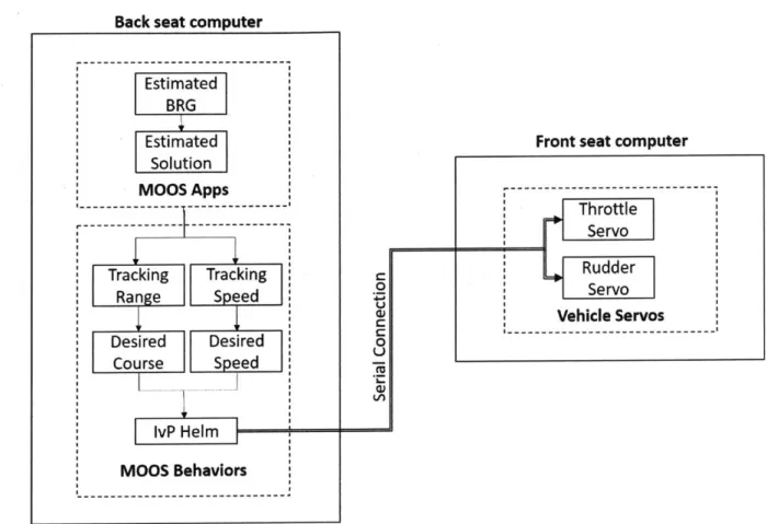
The Jetyak is an impeller driven, modular, three-piece kayak with a Mokai ES-Kape hull, and a Subaru EX21 four-stroke engine [26]. The Jetyak has three operating modes: manned, remote controlled, and autonomous [14]. While in autonomous mode, the Jetyaks utilize a front seat/back seat computer architecture. All helm decisions (i.e. speed, heading, and waypoint calculations) are made by the back seat and controlled with MOOS-IvP autonomy software. The back seat passes this information to the front seat, via a serial command to actuate the throttle and rudder servos. The front seat then, in turn, passes pertinent vehicle information (i.e. vehicle position and speed) to the back seat. This is illustrated in Figure 4-3.

The modular design of the vehicle allows multiple sensors to be easily configured and mounted for many different applications. For the experiments presented in this thesis, each Jetyak was equipped with an eight-element horizontally mounted hydrophone line array to collect and process all acoustic data. The line array is mounted on the port side of both vehicles, approximately 1 meter below the surface. The array is made up of eight

HTI-96-Figure 4-2: One of two Jetyak ASVs used during real-world experiments, collecting acoustic data to demonstrate the effects of range and speed on the RL of the received signal emitted from the source.

MIN hydrophones [10, pictured in Figure 4-4. The analog signals from the hydrophones are converted to a digital signal at a sample rate of 19200 Hz using a Measurement Computing USB-1608FS-Plus-OEM data acquisition board [5], and then stored and processed on a Raspberry Pi 3 Model B computer [19]. This process is illustrated in Figure 4-5. The eight channels were equally weighted, with a nominal array spacing of 9 inches (0.2286 meters). The array specs are summarized compactly in Table 4.1.

Number of Channels 8 Sampling Frequency 19200 Hz

Samples per file 19200 Element Spacing 0.2286 m

Table 4.1: Summary of acoustic array design specifications

4.2

Acoustic Data Collection

4.2.1 JetYak Self-Noise vs. Speed Test

Acoustic data were collected from each vehicle to measure the Power Spectral Density (PSD) of the self-emitted noise at speeds ranging from 0 m/s (engine idling) to maximum

sus-Back seat computer

Front seat computer

--- -- ---

---Throttle Servo

Rudder

Vehicle Servos

Figure 4-3: Flow of information between front seat and back seat computers for autonomous decision-making.

tainable speed (approximately 3.0 m/s, with intermittent speeds up to 3.5 m/s), at speed increments of 0.5 m/s.

The horizontal line array outlined in Section 4.1 was equipped to each vehicle, 1 meter below the surface. One vehicle was operated at a time in autonomous mode and drove the track shown in Figure 4-1, going from the southwest waypoint to the northeast waypoint, turning around, and ending at the southwest waypoint. This procedure was repeated at incremented speeds of 0.5 m/s up to the maximum sustainable speed of approximately 3.0 m/s. Once these data were collected from the first vehicle, the engine was turned off, and the experiment was repeated using the second vehicle.

4.2.2 Source Detection and SNR Experiment

On July 11, 2019 an experiment was conducted off the WHOI pier in Woods Hole, Mas-sachusetts, with two Jetyaks operating in remote-controlled mode, and one Lubell LL916C

Estimated BRG Estimated * Solution MOOS Apps --- --- I --- -- --- --- --Tracking Tracking Range Speed Desired Desired Course Speed lvPHelm MOOS Behaviors 0 0 V I

Figure 4-4: HTI-96-MIN hydrophone [10].

8

7

Watertight Acoustic Bottle:

Raspberry

Pi/Data DAQ

Storage 4

12V Power _{Ba er}

Power

Figure 4-5: Data flow process from eight element hydrophone array to storage on a Raspberry Pi 3 Model B Computer.

underwater acoustic source [16] emitting a continuous 1 kHz tonal. The specifications of the acoustic source are listed in Table 4.2.

During the experiment, both the source and line array were approximately 1 meter below the surface. This experiment was broken up into 2 different tests, each with different vehicle configurations and goals. Figure 4-6 shows the test tracks and configurations for the vehicles and sound source. In the first test, the vehicle operated along a East-Westerly track, while the source was tied to the pier. The goal of the first test is to demonstrate the effects of range and speed on the RL and to test the models that were developed to predict the RL

Source Model Lubell LL916C Output Level 180dB/uPa/m at 1kHz Operating Frequency 1 kHz

Table 4.2: Operating characteristics of Lubell LL916C underwater acoustic source.

(a) (b)

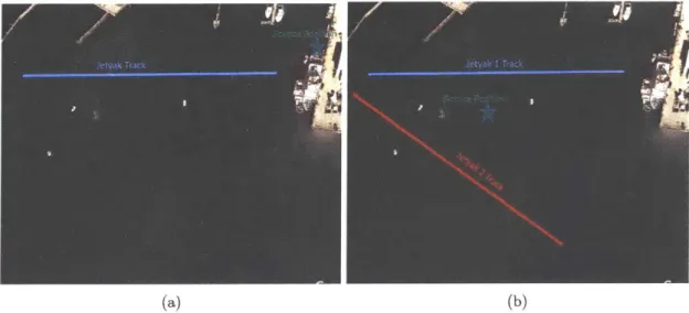
Figure 4-6: Vehicle and Source configurations for the two acoustic experiments performed. (a) Test 1 configuration with vehicle tracks perpendicular to each other and sound source placed at the WHOI pier; (b) Test 2 configuration with vehicles passing fixed sound source in the harbor [6]

for the given speed and range. In the second test, the sound source was tied to a dead in the water (DIW) boat in the harbor and two Jetyaks passed the sound source, on either side. The goal of the second experiment was again to validate the assumed models, but also to demonstrate the ability to deploy a low-cost passive acoustic system on an ASV to detect and track a sound source in the water.

4.3

MOOS-IvP Simulations

A series of simulations were conducted in the MOOS-IvP environment to demonstrate the theoretical capability of ASVs to autonomously localize a target of interest, and adapt their behavior to either track it based on optimizing SNR or intercepting it based on inputs from a collaborator. The simulations were conducted in a shallow water environment, similar to the one observed in Woods Hole Harbor, Massachusetts. In the simulations, the vehicles are divided into one of two categories: one vehicle will be referred to as the "tracking vehicle" and the other one will be referred to as the "intercept vehicle".

4.3.1 MOOSApps

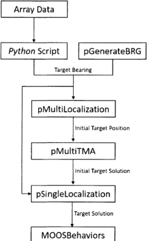
Several MOOSApps that are common to both vehicles were developed to accomplish the goals of this thesis. Figure 4-7 shows a flowchart of the MOOSApps with the inputs and outputs to all of the MOOSApps. In a real-world environment the acoustic data from the

Array Data

Python Script pGenerateBRG

Target Bearing

pMultiLocalization

Initial

pMultiTMA

Initial

- pSingleLocalization

Target Solution

MOOSBehaviors

Figure 4-7: Flowchart of MOOSApps that were developed in support of this thesis

line array is processed in real-time using a Python Beamforming script that was developed in support of this thesis, and the estimated bearing is passed to pMultiLocalization. However in a simulated environment, we do not have real acoustic data to process, so a noise-corrupted simulated bearing is generated via pGenerateBRG and passed to pMultiLocalization.

pMulti-Localization is run on both vehicles and shares the estimated bearing with the other vehicle.

An initial position estimate is then calculated by determining where the bearings cross, as discussed in Section 3.2. This position estimate is then passed to pMultiTMA. After a pre-determined wait interval, pMultiLocalization calculates a new position estimate and passes it to pMultiTMA. Once pMultiTMA has two position estimates it uses the time and position difference to obtain an initial course and speed estimate of the target. The target solution is then passed to pSingleLocalization to initialize the EKF.

future solution estimate updates are done in pSingleLocalization. pSingleLocalization is also run on both vehicles, however the EKF is designed to take either one or two bearings as an input, in the event that one vehicle loses acoustic contact on the target (i.e. the intercept vehicle enters a shadow zone or maneuvers to place the target in forward endfire while clos-ing range to the target).

Finally, once pSingleLocalization has been activated, the vehicles will enter either the

Tracking or Intercept Mode.

4.3.2 MOOSBehaviors

To accomplish the Tracking and Intercept Modes, two MOOSBehaviors were developed:

BHV_ Track and BHV_Intercept. Prior to mission launch, a transmission loss vs range

analysis for the anticipated sound speed profile, source depth, and receiver depth is per-formed using the BELLHOP modeling software [20] and is loaded into BHVTrack. Using the data from BELLHOP, as well as the current solution estimate to the source,

BHVTrack evaluates the course and speed that will result in the highest average SNR

over the next one minute, without resulting in it entering a shadow zone. If the vehicle esti-mates that it is impossible for it to maintain the SNR greater than a set detection threshold during the entire one minute period, the vehicle selects a course and speed that minimizes the time with the SNR below this threshold.

Once the vehicle has arrived at the optimum tracking range, it maneuvers to place the target broadside and matches the target's speed to maintain range.

The BHV_ Intercept behavior uses the current system solution to calculate the shortest path and time to intercept the target of interest, and updates its desired heading and speed to reposition to the calculated intercept point. Throughout the entire tracking process, the tracking vehicle remains in constant communication with the intercept vehicle, continuously providing updated target solutions, to allow the intercept vehicle to update its intercept point even when it no longer holds acoustic contact on the target.

4.3.3 Shallow Water Summer Profile

In a shallow water summer profile, as illustrated in Figure 4-8, sound is more likely to have a boundary interaction than in a deep water environment. As a result, sound is attenuated more quickly, and does not propagate as far. Figure 4-9 shows the transmission loss vs

1

I

Figure 4-8: Shallow water summer profile [13].

range in this environment, with a 1 kHz source placed at a depth of 1 meter, and a receiver placed at a depth of 1 meter. This requires a receiver to be placed at a relatively close range to detect the source. Because of this, the simulation presented began at an initial range within 2000 meters, to ensure that the source would be detectable. In this simulation, the

V" l ,

--235 --

---.'-,,

V

3545 ¶535 5235

Figure 4-9: Transmission Loss vs Range plot for a 1 kHz source at a depth of 1 meter and a receiver at 1 meter.

tracking vehicle began to the southeast of the source, at an initial range of approximately 1100 meters, on a course of 180. The intercept vehicle began to the southwest of the source on a course of 090. Both vehicles had an initial loiter speed of 2 m/s. The initial conditions of the simulation are summarized in Table 4.3.

40~

8-.84

-IG5[

Vehicle Tracking Vehicle Intercept Vehicle Source Course 180 090 270

t

Chapter 5

Results

The analysis and results of two real-world acoustic collection experiments as well as tracking and intercept simulations are presented in this chapter.

5.1

Jetyak Self-Noise vs. Speed Test Results

To determine the speed based noise characteristics of each vehicle, a baseline noise test was performed on March 28, 2019 in Woods Hole Harbor. The results of the experiment described in Section 4.2.1 are presented in this section.

5.1.1 Jetyak 1

To process the data, first the voltage signals received from the hydrophone are converted to a pressure measured in micro-Pascals (pPa) by a conversion factor [10]:

P = 10167/2OV, (5.1)

where P is the pressure and V is the received voltage. Then, a spectrogram of the acoustic data was generated, as shown in Figure 5-1. The spectrogram is generated by taking a discrete Fourier transform (DFT) of windowed time segments [24]. From the spectrogram, we observe that the Jetyak has strong tonals between 80 Hz and 120 Hz, with evenly spaced harmonics out to approximately 800 Hz. The power spectral density (PSD) is then calculated by squaring the magnitude of each DFT time segment and converted to dB using equation

I

Figure 5-1: Spectrogram of acoustic data collected on Jetyak 1 in Woods Hole Harbor, Massachusetts on March 28, 2019.

5.2:

PSDdB = 10logio(PSD), (5.2)

where Pref is 10-6 for water. Finally, a moving average filter was applied to the PSD and speed data of the vehicle to obtain the RL of the noise received by Jetyak 1 at each speed, as shown in Figures 5-2 and 5-3. Finally, the total noise contributed by the Jetyak is calculated by subtracting a reference background noise level of 70 dB. The reference background noise level was determined by finding the average ambient noise level in the water with the vehicle turned off. This reference background noise level is variable depending on several variables, including the wind speed, current, and merchant traffic, and therefore must be determined prior to every experiment.

Figures 5-5 and 5-6 show that the received level is fairly linear for speeds between 1.5 m/s and 3.0 m/s, and the average SNR results for each measured speed are listed in Table 5.1. From linear interpolation, we obtained the expected transmission loss vs speed for Jetyak 2, to be approximately modeled by Figure 5-4.

5.1.2 Jetyak 2

The same process was repeated for Jetyak 2, and resulted in similar results, as shown in Figures 5-5 and 5-6. A summary of the average observed RL vs speed is found in Table 5.2,

Figure 5-2: Raw RL vs. Seedo eyk1

1020

40

2Tk00 2(s) 000 120 420 1400 020

Figure 5-3: Filtered RL vs. Spedo Jtak1

12b2

Iv

0 00 40 Ma a 4M1I IBM

Figure 5-2:Raw Rvs. SpeedofJetyak1.

5 Ru

200 t 00es e2 wer 1cn0 Hle

2--200 49e go0 M0 low 22 1400 20M IND0

Figure 5-3: Filtered RLvs. Speed of Jetyak 1.

again using areference background noise level of 70dB. Again, from linear interpolation, we obtained the expected transmission loss vs speed for Jetyak 2,to beapproximately modeled by Figure 5-7.

5.2

Field Results

A series of real-world tests were conducted on July 11, 2019 in Woods Hole Harbor to

observe the effects of range to the receiver versus the RL at the Jetyak, and to demonstrate the ability to successfully detect a contact of interest on a deployed ASV. Prior to conducting the experiments, a ambient background level of approximately 90 dB was measured, and

I

Table 5.1: Speed vs. SNR results for Jetyak 1.

the~O esiae transissio los vsl speed

5..

et1-~ Sttoaysuc o h okwt

siglvhil

I21

isi

V- i's 2 0 3

Figure 5-4: Linear interpolation of data obtained from Jetyak 1test experiment, modeling the estimated transmission loss vs speed.

was used as the reference level for both Test 1and Test 2.

5.2.1

The first test was conducted with a single vehicle, and a 1 kHz sound source tied off the pier at a depth of approximately 1 meter. As shown in Figure 4-6a, the Jetyak was driving perpendicular to the pier, on an East-Westerly course.

Figure 5-8 shows the RL change over the course of the first test, as the vehicle approached and drove away from the source. This figure also plots the Jetyak speed and range from the source as a function of time. From Figure 5-8, there is a clear inverse relationship between range to the source and RL. However, from this plot, it is not as clear if the change in speed over the course of the test had much impact on the RL. As a result, the expected SNR versus SNR plot, Figure 5-9, was developed to compare the accuracy of the models.

The expected SNR was realized by segmenting the test into 1 second increments to ex-tract the estimated attenuation of the signal due to range from the source (TL) from Figure

7o0o

2D0 4W0 MO we l0ow '2M 1400 2005 $POW 0 0!

Figure 5-5: Raw RL vs. Speed of Jetyak 2.

Fiue5-:FltrdR/v.See fJeyk2

M00 4M0 WO WO 500 12W0 140 050 ISU~

Figure 5-6: Filtered Rbvs. Speed of Jetyak 2.

4-9 and the total background noise (reference background noise of 90 dB plus the added noise from the Jetyak) from Figure 5-4.

The results modeled in Figure 5-9 has an average difference between expected and re-ceived of 1.37 dB and a standard deviation of 4.67 dB. As can be seen in Figure 5-9, at approximately 850 seconds into the test the expected is almost double what the received value was. This is likely due to the ambient background noise level being higher than the 90 dB reference level (possibly due to a noisy vessel starting up). The variability of the ref-erence background noise level limits the accuracy of the models. To obtain a more accurate estimated SNR, additional sensors can be added to the vehicles to continuously monitor background noise levels in real-time.

22,

14-31

Speed (1ft)

Figure 5-7: Linear interpolation of data obtained from Jetyak 2 test experiment, modeling the estimated transmission loss vs speed.

Noise vs. Time 120 110 2100 -100 200 300 400 500 600 700 800 900 1000 Time (s) Range vs. Time 100 50 100 200 300 400 500 600 700 800 900 1000 Tine (s) Speed vs. Time 002 0 100 200 300 400 500 600 700 800 900 1000 Timne (S)

Figure 5-8: RL vs Time plotted alongside Range and Speed vs. Time for Test 1.

J.9yok 21MI I - I GOW&W

-P-24

2,5

Speed (m/s) SNR (dB) Idle (< 0.5 m/s) 10 1.5 22.17 2.0 25.25 2.5 27.7 3.0 29.89

Table 5.2: RL versus speed results for Jetyak 2.

Figure 5-9: Expect~e t " AtamLRsls o et1

0p e i gu 51a 52a te vs t

400 lw 12

Figure 5-9:tExpected vsActual RL Results for Test 1.

5.2.2 Test2- Stationarysourcein theharbor with two vehicles

The second testwasconductedwith a sound source i, te aboat inthe harboriwith both vehicles driving by ona rEast-Westerly course.Once again, the sourcewasemittinga con-tinuous 1 klzsource, as shown in Figure 5-10.

Aswiththe e firstitest, the Rbversus time foreachvehicleis plottedwiththerangeand speed over time in Figures 5-11 and 5-12, and the expected versus the actual Rbis displayed in Figure 5-13 and 5-14. Using the speed models from Figures 5-4 and 5-7, the expected versus measured SNR values were relatively accurate with Jetyak 1having amean difference of 1.16 dB with astandard deviation of 5.82 dB and Jetyak 2having amean difference of 2.39 dB with astandard deviation of 4.01 dB. Again, the high degree of variability in the ambient noise level will require additional noise sensors to beadded to the vehicles to update the reference level in situ as the background noise level increases or decreases.

Now that the ability to detect a contact of interest has been demonstrated, the next step to demonstrate the ability to deploy a passive acoustic system on a low cost ASV to