Recent Advances and Perspectives on Nonadiabatic Mixed Quantum–Classical Dynamics

(1)

HAL Id: hal-01965458

https://hal-amu.archives-ouvertes.fr/hal-01965458

Submitted on 26 Dec 2018

HAL is a multi-disciplinary open access

archive for the deposit and dissemination of sci-entific research documents, whether they are pub-lished or not. The documents may come from teaching and research institutions in France or abroad, or from public or private research centers.

L’archive ouverte pluridisciplinaire HAL, est destinée au dépôt et à la diffusion de documents scientifiques de niveau recherche, publiés ou non, émanant des établissements d’enseignement et de recherche français ou étrangers, des laboratoires publics ou privés.

Recent Advances and Perspectives on Nonadiabatic

Mixed Quantum–Classical Dynamics

Rachel Crespo-Otero, Mario Barbatti

To cite this version:

Rachel Crespo-Otero, Mario Barbatti. Recent Advances and Perspectives on Nonadiabatic Mixed Quantum–Classical Dynamics. Chemical Reviews, American Chemical Society, 2018, 118 (15), pp.7026-7068. �10.1021/acs.chemrev.7b00577�. �hal-01965458�

(2)

1

Recent Advances and Perspectives on

Nonadiabatic Mixed Quantum-Classical Dynamics

Rachel Crespo-Otero1_{* and Mario Barbatti}2_* 1

School of Biological and Chemical Sciences, Queen Mary University of London, Mile End Road, London E1 4NS, United Kingdom.

2

Aix Marseille Univ, CNRS, ICR, Marseille, France.

* Corresponding authors: r.crespo-otero@qmul.ac.uk (RCO); mario.barbatti@univ-amu.fr;

www.barbatti.org (MB)

Abstract

Nonadiabatic mixed quantum-classical (NA-MQC) dynamics methods form a class of computational theoretical approaches in quantum chemistry, tailored to investigate the time-evolution of nonadiabatic phenomena in molecules and supramolecular assemblies. NA-MQC is characterized by a partition of the molecular system into two subsystems, one to be treated quantum-mechanically (usually, but not restricted to electrons); and another to be dealt with classically (nuclei). The two subsystems are connected through nonadiabatic couplings terms, to enforce self-consistency. A local approximation underlies the classical subsystem, implying that direct dynamics can be simulated, without needing pre-computed potential energy surfaces. The NA-MQC split allows reducing computational costs, enabling the treatment of realistic molecular systems in diverse fields. Starting from the three most well-established methods—mean-field Ehrenfest, trajectory surface hopping, and multiple spawning, this review focus on the NA-MQC dynamics methods and programs developed in the last ten years. It stresses the relations between approaches and their domains of application. The electronic structure methods most commonly used together with MQC dynamics are reviewed as well. The accuracy and precision of NA-MQC simulations are critically discussed, and general guidelines to choose an adequate method for each application are delivered.

(4)

3

1 Introduction

Photochemical and photophysical phenomena in molecules, supramolecular assemblies, and solids involve the time evolution of the electronic population through a manifold of electronic states. Modeling these processes requires considering the coupling between the nuclear and electronic motions beyond the adiabatic regime. The high computational costs of such simulations have led to the development of different strategies. On the one hand, it is possible to tackle the problem fully quantum mechanically but at reduced dimensionality by exclusively treating, for instance, the electron dynamics in a frozen nuclear frame or incorporating few nuclear modes. On the other hand, full dimensionality may be retained at the cost of splitting the system between a set of degree of freedom to be treated fully quantum mechanically and another set to be treated classically. This second strategy is the basis of the Nonadiabatic Mixed Quantum-Classical (NA-MQC) dynamics explored in this review.

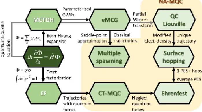
NA-MQC dynamics is a general umbrella under which we may classify several different approaches developed to deal with time-resolved simulations over the last forty years. Among these approaches, we may include trajectory surface hopping (TSH), mean-field Ehrenfest (MFE), mixed quantum-classical Liouville equation (QCLE),1-3 the mapping approach,4-5 multiple spawning (MS),6-7 nonadiabatic Bohmian dynamics (NABDY),8-9 and the recently proposed coupled-trajectories mixed quantum-classical (CT-MQC) method.10 Naturally, as in any classification, there is a degree of arbitrariness: should MS be still considered an NA-MQC approach, as it ultimately recovers the information on the nuclear wave packet? We broadly define the NA-MQC methods as those propagating the nuclei (or more generally, slow particles) via classical trajectories. We believe, however, that it is not productive to focus on such a taxonomic question. In the interest of pragmatism, we instead assume some porous boundaries and discuss methods that incorporate full dimensional treatment of electrons and nuclei, the inclusion of nonadiabatic transitions, and some type of classical/quantum partition. Fig. 1 schematically illustrates the hierarchic relation between some of the key methods for nonadiabatic dynamics.

With this definition in mind, we prepared this review focusing on methods, rather than on applications. Nonetheless, it would be yet a Homeric work to attempt to survey all classes of NA-MQC methods. For this reason, we have narrowed our focus even further to NA-NA-MQC methods often used in conjunction with direct (or on-the-fly)11 calculations of electronic structure properties

(5)

4 (in opposition to methods that have been mostly applied with model Hamiltonians). In the last fifteen years or so, on-the-fly NA-MQC dynamics has been pushing the boundaries of excited-state computation chemistry, becoming a central tool for investigating practical problems in diverse fields.6, 12-15

In the sub-class of on-the-fly NA-MQC methods, we first examine the three cornerstone approaches—mean field Ehrenfest, trajectory surface hopping, and multiple spawning (Section 2.3). From them, we guide the reader through a myriad of new methods that have been developed, especially in the last decade (Section 3). The equations of motion (EOM) for the main methods are written out, sharing a standard notation to emphasize the relations between them. The used symbols are outlined in Table 1.

Due to the narrow focus, with few exceptions, we will not discuss methods related to NABDY, QCLE, and the mapping approach. The first class is reviewed in Ref.16. An excellent introduction to the latter two classes of methods can be found in Ref.17. Concerning QCLE, we also recommend Ref.18 for details on the momentum-jump (MJ) QCLE and the generalized quantum master equation (GQME) approaches.

Fig. 1 Schematic relation between methods for nonadiabatic dynamics. Starting from the exact non-relativistic time-dependent Schrödinger equation (center, left), the full molecular problem may be solved either via a Born-Huang expansion (as done in MCTDH), an exact factorization (EF) of the molecular wavefunction, or propagation of the density via Liouville equations. In the Born-Huang branch, MCTDH combined with Heller’s frozen Gaussian wave packets (GWP) approach renders the vMCG approximation, which, in the limit of a coherent GWPs, converges to Multiple Spawning (MS).19_{In the EF branch, a trajectory approximation of the nuclear wave packet leads to the}

CT-MQC method, in which trajectories are coupled by quantum forces. If these quantum forces are neglected, the method reduces to the mean field Ehrenfest (MFE) approach.10_{The connection between MFE and vMCG is discussed in Ref.} 20_{. If instead of propagating the trajectories on an average potential energy surface, they are propagated on a single}

surface, which can be stochastically exchanged by another, surface hopping (TSH) is recovered. In the third branch, the quantum density is propagated via Liouville equations. The mixed-quantum-classical limit of the partial Wigner trasform of the density gives rise to the quantum-classical Liouville equations (QCLE). From QCLE, assuming unique trajectories, large nuclear velocities, and modifying the electronic density matrix leads to fewest switches TSH.21_If

(6)

5

propagating the nuclei through classical trajectories, which includes multiple spawning, CT-MQC, Ehrenfest, QCLE, and surface hopping. This chart presents some of the main approaches in the field, but it is far from representing the broad variety of alternatives available.17, 22

The importance that on-the-fly NA-MQC dynamics has acquired in computational chemistry rests on how general it became thanks to interfaces between dynamics algorithms and general electronic structure methods. We cover this relation as well, discussing the leading electronic structure methods that have been employed for NA-MQC simulations (Section 4). At this point, we prefer to assume a critical perspective, focusing our account on the limitations and potential problems of each of these methods.

Table 1. Table of symbols recurrently used in the text.

Symbol Definition

 Molecular wavefunction

K Electronic wavefunction

 Nuclear wavefunction

,  Slater determinant, molecular orbital, atomic orbital cK, AK Electronic and nuclear time-dependent coefficients

 Density matrix

SJK Wavefunction overlap

ˆ

H, ˆH _e Molecular and electronic Hamiltonian ˆ

n

K , ˆK e Nuclear and electronic kinetic energies ˆT,ˆ Cluster operator, excitation operator Ee, EK Electronic energy, adiabatic energy

 Potential

F, G Force, energy gradient

NAC JK



Time-derivative nonadiabatic coupling SOC

JK

 ,



_JKEMC Spin-orbit coupling, radiation-matter coupling dJK Nonadiabatic coupling vector

JK, fJK Transition dipole moment, oscillator strength I, J, K, L Index for electronic states; L is the active state

 Index of nuclei

N Index for trajectories of ensemble points i, j; a, b Indexes for occupied and unoccupied orbitals

R, r Nuclear and electronic coordinates

v, P, M Nuclear velocity, momentum, and mass

ˆ ,

A A Classical value and operator of observable A

t,  Time, decoherence time

(7)

6 The development of time-resolved spectroscopy has revolutionized the way we explore chemical systems.23-26_{The information delivered by these experimental methods, however, needs}

to be deconvoluted, which has raised the importance of computational chemistry. Theoretical simulations are now vital ingredients for the analysis of any advanced experimental set of data; and NA-MQC dynamics plays an important role for that, naturally providing time-resolved information. In Section 5, we discuss how NA-MQC dynamics has been used to simulate several spectroscopic techniques directly.

With the popularization of the NA-MQC methods, several computational programs dedicated to NA-MQC dynamics (or having NA-MQC dynamics incorporated as an auxiliary algorithm) have been developed and released in the last ten years or so. We are ourselves developers of one of such programs, the Newton-X platform. In Section 6, we survey these implementations, but we already anticipate this part of the review will be quickly outdated, given the frenetic rate of new developments released nowadays.

NA-MQC dynamics comes at a cost. Hundreds of thousands of CPU hours may be required to simulate a single molecule. Researchers have coped with such cost by both developing new optimized techniques and downgrading theoretical levels. The price to pay for this second strategy may be too high, leading to unacceptable loss of accuracy. This problem is discussed in Section 7.

As specialists in the field, developing a major program platform for NA-MQC dynamics and applying these methods to investigate many different systems, we have accumulated an experience that we believe may be useful to share. Throughout the review, especially in Section 8, we lay down a series of recommendations on methods and procedures. We hope they will be useful not only for beginners in the field but also for experienced researchers, who may re-evaluate their own choices. Naturally, these are educated but somewhat subjective opinions. The reader will always be warned when this is the case.

2 Standard methods for NA-MQC dynamics

Three of the most traditional NA-MQC dynamics methods for treating nonadiabatic phenomena are the MFE, SH, and MS. Each of them tackles the nonadiabatic process in an entirely different way either by averaging electronic states (MFE), hopping between states (TSH), or spawning new basis functions to other states (MS). These methods have been discussed and

(8)

7 reviewed in detail in Refs. 16, 27-32_{. In this section, we only outline their main features, which will}

be useful to discuss the new developments that have been recently proposed.

In common, these three types of methods share a treatment of nuclear motion in terms of classical trajectories (which in the case of MS are used as an auxiliary grid for a quantum propagation of the nuclei). As a consequence, at each time step of a trajectory evolution, they require computation of electronic quantities (potential energies, energy gradients, couplings, etc.) for the classical position of the nuclei (local approximation). Such approximation has a significant impact on computational costs because pre-computed multidimensional surfaces for electronic coordinates are not required anymore. Instead, these methods may be implemented as to compute these quantities on-the-fly during the trajectory integration. Naturally, the classical localization of nuclei is also the drawback of these methods, as they fail to provide a description of quantum phenomena depending on global features (like tunneling, for instance).

2.1 Mean-Field Ehrenfest Dynamics

We start with the time-dependent Schrödinger equation (TDSE)

ˆ

i H

t

 _{ }

 (1)

where  is the total (non-relativistic) molecular wavefunction. The full Hamiltonian in this equation is taken as

ˆ ˆ _{ˆ ,}

n e

H K H (2)

where ˆK is the kinetic energy operator for the slow particles (usually nuclei) and ˆ_n H is the e Hamiltonian for the fast particles (usually, but not necessarily only electrons33-34_).

In the mean-field approximation, the molecular wavefunction is factorized in terms of a function of coordinates r describing the fast particles and a function of coordinates R describing the slow particles:35





   

0 , , , , exp ' ( ') , t e t i t  t t dt E t      _ _ 



 r R R r (3)

(9)

8 where the phase factor is E_e  Hˆ_e  .

Fig. 2 Schematic illustration of the mean field Ehrenfest (MFE) dynamics. A trajectory is run on a surface averaged over all electronic states weighted by their respective electronic population.

After replacing this wavefunction Ansatz, Eq. (3), in Eq. (1), the TDSE can be projected in the fast-coordinates space and in the slow-coordinate space leading to two coupled time-dependent equations for  and . The classical limit ( 0) of the equation for  can be easily shown35 to be equivalent to Newton’s equations for the motion of each slow particle



(with classical coordinate R and mass M_) on the average potential of the fast particles:

 

2 2 1 , d dt M_ R F R (4) where

 

_, ˆ

 

_;

 

_, _. e t H t      r F R r r R r (5)

The fast particles, in turn, evolve according to



, ;



_ˆ

_{  }

_

; , ; , e t i H t t     r R r R r R (6)

where we have made explicit the parametric dependence of the electronic wavefunction on the classical nuclear coordinate. (For the complete derivation of Eqs. (4) and (6), see Ref.16.)

(10)

9 The classical equation of motion (EOM), Eq. (4), can be integrated with standard methods, as the velocity Verlet algorithm.36_{The quantum EOM, Eq. (6), can be solved numerically along}

the classical trajectories without a need of choosing basis functions. Alternatively, if the fast particles correspond to electrons, the time-dependent electronic wavefunction



can be expanded as a linear combination of electronic states:



, ;



K

 

K

 

; ,

K

t c t 

 r R 



r R (7)

where  are electronic wavefunctions for state K, with parametrical dependence on the classical _K nuclear coordinates R

 

t . If this multiconfigurational approach is used, the quantum EOM (Eq. (6)) is reduced to35 . NAC J K JK JK K dc i c H dt      _  _  



(8) In this equation,

 

ˆ JK J e K H R   H  (9) and

 

. NAC K JK J JK t         R d v (10)

In the last equation,

JK  J K

d (11)

is the nonadiabatic coupling (NAC) vector and v is the classical nuclear velocity. The coefficients J

c define a density matrix ρ whose diagonal terms * JJ c cJ J

  are the populations, and the off-diagonal terms *

IJ c cI J

  are the coherences.

Still with the expansion in Eq. (7), the force acting on the nuclei is

 

* ˆ . I J I e J IJ c c  H   



 F R (12)

(11)

10 Particular expressions for the force in the adiabatic and diabatic representations are given in Eqs. (29) and (30) of Ref.37_{. The implementation of a second-order Ehrenfest method based on}

CASSCF, in which Hessian information is used to increase integration time steps in the classical EOM, is discussed in Ref.38.

To summarize, in MFE, the system is propagated by simultaneously solving the quantum EOM for the classical coordinates R, Eq. (8), to obtain the matrix elements of c; and the classical EOM, Eq. (4) with the average force in Eq. (12), to obtain R . The nuclear motion on the averaged potential energy surface is schematically illustrated in Fig. 2.

Because of the average description of the potential, MFE dynamics cannot represent different physical situations found when a system leaves regions of strong NACs. Moreover, MFE does not satisfy the principle of detailed balance,35, 39 which means that at equilibrium a forward process is not balanced by its reverse process. The inclusion of quantum corrections through a modified symmetric coupling matrix element may produce Boltzmann distributions in the long-time limit.40-41 This approach, however, is restricted to propagation in the diabatic representation. The MFE approach, with emphasis on its more recent multiconfigurational variants, has been recently reviewed in Ref.22_{(see also Section 3.2.5). We further discuss the MFE approach in the}

context of real-time single-reference methods in Sections 4.2.4 and 4.2.5.

2.2 Trajectory Surface Hopping

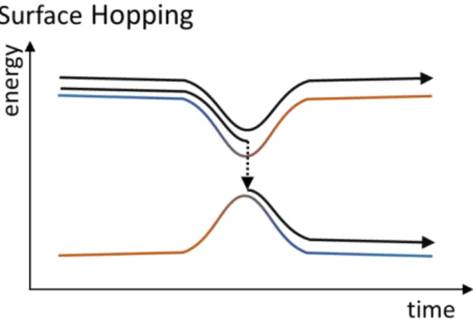
In trajectory surface hopping (TSH), sometimes also called molecular dynamics with quantum transitions (MDQT),42 a swarm of classical and independent trajectories approximates the evolution the nuclear wave packet evolving on individual Born-Oppenheimer (BO) surfaces. Nonadiabatic transitions are considered using a stochastic algorithm to decide whether the system will stay on the current electronic state or hop to another one (Fig. 3).43 Because of its conceptual simplicity and straightforward implementation, TSH is likely the most popular NA-MQC method.

(12)

11

Fig. 3 Schematics illustration of trajectory surface hopping (TSH). An ensemble of independent trajectories is propagated on single BO surfaces. Random events allow trajectories to change the surface mainly at coupling regions.

Although TSH has been in use since the early 1970s, it was only in 1990 that it gained its most famous formulation, the fewest-switches surface hopping algorithm (FSSH).43 In this approach, the electronic time-evolution is obtained via the quantum EOM given in Eq. (8) (the same one used in MFE), while the nuclear dynamics for each nucleus  is propagated on a single BO potential energy surface (PES) of a state L

2 2 1 . LL d H dt M       R (13)

(In an adiabatic basis, H_LL is simply the adiabatic energy E_L.)

During the propagation, the instantaneous probability that the trajectory will nonadiabatically hop from state L to a state J is given by

























1 * * 2 1 2 max 0, Im Re 2 max 0, Im Re , FSSH NAC L J LJ J L LJ J L L NAC LJ JL LJ JL LL t P H c c c c c t H          _              _  _   (14)

(13)

12









* 2 2 max 0, Re 2 max 0, Re . FSSH NAC L J LJ J L L NAC LJ JL LL t P c c c t       _{ }              _ _   (15)

Whether a hopping event from L to J happens or not is estimated by sampling a random number r_t

([0,1]) and evaluating the following condition: 1 1 1 . J J FSSH FSSH L K t L J K K P r P       



(16)

In addition to the inequality (16), some criterion for the conservation of energy is also generally imposed, usually by rescaling the velocity after the hopping in the direction of the NAC vector by a value corresponding to the potential energy gap at the hopping time.44 The rescaling in the NAC directions is motivated by the Pechukas force occurring during the nonadiabatic transition.2, 45-46 If NAC vectors are not available, the velocity is sometimes rescaled in the direction of the momentum, which is an ad hoc procedure to grant energy conservation without further justification. If no scaling can enforce energy conservation, the hop event is not allowed (forbidden or frustrated hop).35 For a discussion on how to treat the momentum in case of forbidden hops, see Ref.17, P. 279-280, and references therein. In the method variant named fewest switches with time uncertainty (FSTU), the Heisenberg uncertainty principle is invoked to allow the classically forbidden hop to occur at a nearby geometry.47

In practical terms, the integration of the quantum and classical EOMs (Eq. (8) and Eq. (13) ) is not done with the same time steps. While the classical EOM requires time steps of about 0.1 to 0.5 fs, the fast oscillations in the quantum EOM require much shorter steps, 0.005 to 0.01 fs. If energies, forces, and nonadiabatic coupling were to be computed at shorter steps as every 0.005 fs, NA-MQC dynamics would not be possible due to the computational costs. Thus, commonly, these electronic quantities are calculated only at the classical steps. The values used for integration of the quantum steps are given by interpolation between subsequent classical steps.

Despite its success, FSSH is an ad hoc theory, not directly derived from first principles. Subotnik and coworkers21_{and, later, Kapral}48_{have recently discussed how FSSH can be connected}

(14)

13 more recently by Markland.18_{In Ref.}21_{, it is shown that FSSH can be approximately derived from}

QCLE provided that two major conditions are satisfied: first, the nuclei should be moving quickly; and secondly, there are no explicit interference effects between nuclear wave packets. In addition, decoherence corrections based on forces differences must be considered as well, an element missed in the FSSH formulation discussed above (see Section 3.1.1). The connection of FSSH to QCLE has also been applied to derive formal ways to evaluate diabatic populations, and expectation values for a TSH propagated in adiabatic representation, as well as to generate initial conditions for an electronic state that is not an adiabatic wavefunction at time zero.50

Different from MFE, FSSH in the adiabatic representation approximately satisfies the principle of detailed balance.51-52

2.3 Multiple Spawning

The multiple spawning (MS) method6-7 expands the nuclear wavefunction by Gaussian functions that are propagated as classical trajectories. In its exact formal framework, MS is also known as full multiple spawning (FMS). When MS is connected to a particular electronic structure method, it is commonly called ab initio multiple spawning (AIMS).

In MS, the number of nuclear functions (NK

 

t ) is allowed to change through spawning events, to represent the bifurcation of the wave packet in regions of significant nonadiabatic couplings (Fig. 4).53-54 Historically, the first on-the-fly NA-MQC simulation based on an ab initio method was done with MS employing generalized valence bond (GVB) wavefunctions.55 (One year before, an on-the-fly TSH had been reported but based on a semiempirical method.56₎

(15)

14

Fig. 4 Schematic illustration of multiple spawning (MS). A classical trajectory serves as the center for a generalized Gaussian wave packet. In the coupling region, new Gaussians may be created to explore other surfaces.

The derivation of MS starts from a Born-Huang expansion of the total wavefunction



, ,



_K

  

, _K ;



. K

t  t 

 r R 



R r R (17)

The nuclear wave packet  is written as a linear combination of multidimensional frozen _K Gaussian functions m

K

g with time-dependent coefficients m K

A and N_f degrees of freedom:

 



 

   



1 , ; , , , , K N t m m m m m m K K K K K K K m t A t g t t t     



R R R P (18) where





2 /4





2 ₁





₁



; , , exp . f N m m m m m m m K K K K K K K g    i i       _ _        R R P R R P R R (19)

The Gaussian widths ( ) are time-independent parameters,57_{the nuclear phase (} m K  ) is propagated semiclassically53, 58

 

3

 

2 1 , 2 m m N Ki m K KK K i i P H t M    _{ } _  R



(20)

and the position-momentum Gaussian centers (Rm_K and P_Km) are propagated classically

 

, . m m K K m m K KK K d dt M d H dt      R P P R (21)

Eqs. (17) and (18) are inserted into the TDSE (Eq. (1)), which is then projected on a particular state (J, m), resulting in an EOM for A_J:

 

1 , J JJ JJ JJ J JK K K J d i i dt   _ _    __  _  _ 



 A S H S A H A (22)

(16)

15 where the matrix elements are given by _{Il Jm}_,  g gl_I m_J _IJ

R S , , l m Il Jm gI gJ IJ t



   R S , and , ˆ ˆ _, l m Il Jm I I n e J J H  g K H g 

R r. The evaluation of the Hamiltonian matrix elements is the

bottleneck of MS simulations. A zero-order saddle point approximation (SPA) is assumed to calculate these integrals:53

 

, ˆ , I l m l m I I J J IJ J l m I J IJ g g g g g g     R r R R O O R O R (23)

where R is the centroid of the product of the functions g_Il and g_Jm. This approximation allows calculating the required parameters on-the-fly. The SPA is applied to compute adiabatic energies

 

I

E R and nonadiabatic couplings d_JK

 

R . Because both should be determined at the centroid

R , it implies that additional electronic structure calculations should be done at each time step. A bra-ket approximation (BAT), which only uses quantities computed at R, has been proposed in the zeroth59 and first order60 to reduce these costs.

The most prominent feature of the MS approach is the spawning of new basis functions to represent the wavefunction bifurcation after leaving the region of significant nonadiabatic coupling. The spawning algorithm is explained in details in Ref.53. At each time step, nonadiabatic couplings d_JK (appearing within H_IJ) for all nuclear basis functions are calculated. Each basis function can spawn new Gaussians when regions with large effective coupling eff

JK JK

  R d (for adiabatic representation) are found. Two parameters, 0 and  , are defined to set the limits of f the region of large effective coupling. These parameters are system dependent and are defined by running test calculations. As soon as eff ₀

JK 

  , the parent basis function is classically propagated (Eqs. (21)) until the condition eff

JK f

  indicates the end of the large effective coupling region. Then, a predefined number of basis functions is evenly spawned in this region (with one of them necessarily at the point with largest eff

JK

 ). In general, the new function is spawned on a different potential energy surface, but it is also possible to spawn new functions on the same electronic surface to simulate tunneling.53

(17)

16 The spawning concept has been the inspiration for other adaptive basis set approaches as the ab initio multiple cloning based on multiconfigurational Ehrenfest (AIMC-MCE),60_{which is}

discussed in Section 3.2.5.

In contrast to TSH, MS solutions can converge to the exact solution if an infinite basis is considered and the matrix elements are entirely computed.19 Their limitations are associated with the truncation of the basis and the use of the local approximations in the evaluation of the integrals.

3 Recent advances in NA-MQC dynamics

3.1 Nonlocal effects in NA-MQC

3.1.1 Incorporating Decoherence

The propagation of the semi-classical TDSE (Eq. (8)) in MFE or TSH is entirely coherent. This means that the electronic coherences—the off-diagonal terms of the density matrix *

IJ c cI J

 

—do not vanish during the dynamics. This problem has long been recognized42, 61-62_{and has been}

the central focus of developments in NA-MQC methods since then. It affects MFE and TSH, but not MS, which adequately addresses it. The decoherence problem has been recently reviewed by Subotnik et al. in Ref.29_.

When the FSSH was proposed, it was thought that the stochastic nature of the algorithm, with each independent trajectory hopping at a different point in the phase space, would be enough to enforce decoherence over the average of the trajectories.43_{Nevertheless, this stochastic effect is}

not sufficient63 and the overcoherence leaves clear effects on TSH results, as, for instance, in the form of substantial divergences between the average of the electronic populations *

II c cI I

  and the number N_I of trajectories in each state.64-65 In other words, the equality

   

*

 

1 1 , Trajs N i I I n trajs trajs N t c t c t N  N 



(24)

which expresses the internal consistency of the algorithm, is not usually satisfied. Thus, because of the overcoherence, the nonadiabatic distribution of the trajectories deteriorates after passing multiple times through regions of significant nonadiabatic couplings.66 Decoherence corrections

(18)

17 have been shown to be essential to render reliable surface hopping dynamics.21_{In more}

fundamental terms, Ouyang and Subotnik have shown that decoherence corrections set the Poincaré recurrence time to infinity, increasing the FSSH accuracy.67 (In a different context, Bastida et al. have derived hopping algorithms constrained to satisfy Eq. (24)68; see Section 3.2.3.) The overcoherence is a direct effect of the nuclear localization at the classical coordinates. When the nuclear wave packet separates in different states after crossing a region of significant nonadiabatic couplings, their overlap and the nondiagonal terms of the density matrix should quickly vanish. This does not happen in MFE or TSH, where the amplitudes of the ghost states (

K

c with KL) are propagated along the same classical trajectory computed for the active state L. The overcoherence can also be understood as consequence of a lack of correlation in a mean field approach.69

Several ad hoc schemes have been proposed to include decoherence in each independent trajectory (see Refs.29, 66_{and references therein). The most straightforward treatment is to assume}

that decoherence is instantaneous and reset the wavefunction to

0, , 1, K L c K L c     (25)

whenever a hop to state L happens.70 The instantaneous decoherence (ID) approach has been evaluated in Ref. 65, where Nelson et al. show that it does not lead to internal consistency (Eq. (24) ). The ID wave-function re-setting in Eq. (25) is on the basis of more involved methods, as the augmented FSSH (A-FSSH)71 and the decoherence-induced SH (DISH).72-73

Zhu, Truhlar, and co-workers have pioneered in the development of energy-based decoherence corrections (EDC), proposing a series of decay-of-mixing (DM) approaches for MFE and TSH.74-76_{An approximated version of the nonlinear DM (SDM for simplified decay of mixing)}

approach developed by Granucci and Persico64_{for TSH has become extremely popular due to its}

simplicity, low computational cost, and the ability to enforce internal consistency (Eq. (24)). In this approach, at each time step after integrating the semi-classical TDSE, the coefficients c_I are corrected according to

(19)

18 / 1/2 2 , , 1 . KL t new K K new L new L K K L L c c e K L c c c c          _  _ 



 (26)

In these equations, L is the active state and the decoherence time  is given by the _KL phenomenological equation 1 1 , K L SDM KL n E E C K        _  _   (27)

where E_I is the potential energy of state I, K_n is the classical kinetic energy of the nuclei. C and



are parameters whose recommended values are 1 and 0.1 Hartree, respectively.74_{With such}

values, the decoherence time for a 1-eV energy gap and 1-eV kinetic energy is approximately 1 fs. Nelson et al.65 have benchmarked the effects of the SDM (and of the original nonlinear DM) corrections to TSH, and tested the dependence on the two parameters.

While the decoherence time in Eq. (27) arose from a phenomenological analysis, a more formal derivation from the overlap evolution of frozen Gaussian wave packets have shown that this time should be proportional to the difference between the forces in different states,61_i.e.

1 1 . K L ODC KL   F F (28)

Such insight has given rise to a series of overlap-based decoherence corrections (ODC), which are based on approximated estimates of wave packet overlap decay. Granucci and Persico,66 for instance, have proposed an ODC approach dependent on two parameters, the wave packet width and the minimum overlap threshold.

The A-FSSH algorithm from Subotnik’s group, in turn, propagates an auxiliary set of coordinates to estimate the overlap decay without any open parameters.29, 63, 77_{Supposing that}

decoherence events can be described by a Poisson process, a stochastic algorithm is invoked to destroy the coherence of a specific state I in favor of the active state L according to

(20)

19 1/2 2 2 , , , 0, . new K K new I new L L L I L c c K I K L c c c c c c         _  _ (29)

The A-FSSH method is significantly more expensive than the traditional FSSH, and recent modifications have been proposed to speed up these calculations.71 A new development, named simultaneous FSSH (S-FSSH), improves the description of the decoherence with the explicit propagation of wave packet widths.78 Transition rates for a one-dimensional spin-boson model are benchmarked with A-FSSH and FSSH against Marcus rates in Ref.77.

This class of ODC approaches has been generalized by Gao and Thiel,79 who derived a non-Hermitian equation-of-motion (nH-EOM) approach for the full density matrix evolution, starting from the Born-Huang expansion for the molecular wavefunction (Eq. (17)) and adopting a polar form for the nuclear wavefunction. In this way, a dissipative term responsible for decoherence and proportional to the quantum nuclear momentum is naturally introduced in the TDSE. The quasiclassical limit of this method can be obtained with frozen Gaussian functions and treated in the frame of surface hopping (nH-SH). A similar approach has been derived by Ha, Lee, and Min based on an independent-trajectory approximation of the exact factorization.80

A decoherence time in the form of Eq. (28) has also been used in non-ODC approaches for NA-MQC as well, like the coherence penalty functional (CPF) for MFE69_{and DISH.}72_{In the case}

of CPF, a new term proportional to 1 KL

 _{is included in the Hamiltonian, penalizing development of} coherences. DISH, on its turn, innovates by using decoherence as the hop criterion.

The methods reviewed in this section rely on the independent trajectory approximation and aim at correcting the overcoherence in individual trajectories. The decoherence problem, however, can also be addressed at the ensemble level, through coupled-trajectory methods. This class of methods will be discussed later (Section 3.2.4).

3.1.2 Incorporating Tunnelling

One of the main challenges for NA-MQC simulations is the treatment of quantum phenomena beyond nonadiabatic effects. In particular, including tunneling has proved to be a

(21)

20 challenging task. Because of their high computational cost and lack of generality, none of the existing algorithms is still in routine use.

In the context of MS, tunneling is considered by spawning new functions in the same electronic state.53 The particles are identified as tunneling, donors, and acceptors; and their identity can change during the simulations. The tunneling vectors (for all donor-acceptor combinations) are defined optimizing the system to their local minima. Tunneling thresholds (minimum donor-acceptor distance) allow detecting when tunneling events can occur in analogy to the spawning threshold, while the direction of tunneling is defined using a straight-line path. When a turning point is found, the basis functions are displaced along the tunnel path. Details of the implementation and applications can be found in Refs.53, 81.

A method inspired by the MS, the ab initio multiple cloning (AIMC) approach (see Section 3.2.5), considers an Ehrenfest wavefunction with the nuclear part described by a Gaussian coherent state.60, 82 Two configurations are generated to describe the bifurcation of the wave packet in the regions of strong nonadiabatic couplings. This cloning approach was recently extended to describe tunneling of hydrogen atoms, with the cloning at the turning points of the potential barrier.82

Truhlar’s group proposed the army ants method to sample rare events in NA-MQC.83_The

recent version of the algorithm, the army ants tunneling method, allows exploring regions of the phase space reached only by tunneling.84_{It has been generalized for its use in nonadiabatic}

dynamic simulations in particular with Ehrenfest method, but in principle can be extended to TSH.85_{The tunneling coordinate (or a combination of two) is defined using internal coordinates}

beforehand. So calculations need to be preceded by careful exploration of the PES. An initial ensemble of trajectories is chosen, and the probability of tunneling is calculated when a turning point is reached according to a Wentzel-Kramers-Brillouin approximation (WKB):

max 0 2 exp 2 ( ) ( ) . WKB P E E d    _      _  _    



q q0  (30)

In this equation,  is the distance in iso-inertial coordinates (scaled to a reduced mass ) at q with respect to the starting point q₀ along the tunneling path. _max_{is the length of the tunneling path.}

E is the mean (adiabatic or diabatic) PES. The rate of change of the coefficients c_J (Eq. (8)) during the tunneling path are given as

(22)

21 1 1 2 ( ) ( ) J J dc dc d  _ __E __E _ dt  q q0  (31)

A probabilistic algorithm is used to decide whether the system will tunnel or not. The population of the trajectories is modulated according to the tunneling probability. Details of these algorithms can be found in Refs.84-85.

The potential of the army ants tunneling has been shown in a recent study for phenol photodissociation dynamics considering the combined effect of coherence, decoherence, and multidimensional tunneling. These simulations show the bimodal nature of the kinetic energy spectra.86

Methods based on path integral formulation, such as ring-polymer molecular dynamics (RPMD),87 taking into account quantum behavior of quantum particles can include the effect of zero-point vibrational energy and tunneling. Recent implementations of these methods with Ehrenfest and TSH schemes for the electronic represent an alternative for the treatment of such quantum effects, as discussed below.88-91

In RPMD, quantum particles are mapped onto a closed flexible polymer of P beads, profiting from an isomorphism between the quantum-statistical problem formulated in terms of a discretized version of Feynman's path integral and a classical problem. RPMD is derived for equilibrium processes, its use for non-equilibrium processes such as excited state dynamics, is done ad hoc. Sushkov, Li, and Tully90_{developed a nonadiabatic version of RPMD in the frame of}

FSSH (RPSH). In their approach, the ring polymer is interpreted as an effective molecule moving on an effective potential energy surface coupled by NACs. With such formulation, they have proposed two different models for an effective semiclassical TDSE (Eq. (8)), which is employed for FSSH. The method is aimed at the treatment of systems with quantum and near-classical degrees of freedom and was specifically tested for computation of reaction rates with a significant contribution of tunneling.

Lu and Zhou88 have developed a conceptually different version of RPMD with TSH named path integral molecular dynamics with surface hopping (PIMD-SH). While in the RPSH the ring is treated as a molecule (each bead is an atom) that moves on a single potential energy surface, in the PIMD-SH, each bead may occupy a different state, directly related to the actual electronic

(23)

22 states. The aim of the PIMD-SH method has been to sample equilibrium distributions to compute thermal averages for observables.

In Ref.8, Tavernelli derives a nonadiabatic Bohmian trajectory-based quantum dynamics (NABDY), which can treat tunneling problems. In this approach, the trajectories evolve under the action of adiabatic and nonadiabatic quantum potentials, dependent on the other trajectories, which make the dynamics exact in principle.

3.2 New approaches to NA-MQC

3.2.1 Dynamics near intersections

The nonadiabatic coupling matrix in Eq. (10) can be written as

ˆ , J e K JK J K K J H E E          d (32)

where E_I is the adiabatic potential energy of state I. Near state crossings (E_K E_J), the coupling diverges producing a steep cusp. In practical terms, the actual intersection (E_K E_J)—where the coupling diverges, and the calculation of hopping probabilities breaks down—is a rare event, and usually does not pose a problem for most of the trajectories. Nevertheless, the steep shape of the nonadiabatic coupling may be missed during the trajectory propagation, if the time steps are too large (Fig. 5).92 Take, for instance, the results for CNH4+ from Ref.93. They show that the NAC is

significant in a narrow range of about 0.1 rad around the twisted geometry. Given that the excited-state torsional period for this molecule is about 40 fs, strong couplings are restricted to a time window of about 0.6 fs, which is of the same order as the time steps typically employed for the integration of Newton’s equations (0.1 – 0.5 fs).

This problem is even maximized in supramolecular assemblies, where the high density of states causes many state crossings due to localized adiabatic states lying in monomers far away in the space, and, therefore, not contributing to the electron dynamics. This type of crossing has been called trivial or unavoided crossings.94_{In trivial crossings, the NAC shows an even sharper peak}

(24)

23 easily missed during numerical integration. As a result, artifacts may occur due to an improper change of diabatic character of the active state.

Fig. 5 Schematic illustration of the adiabatic energies and nonadiabatic couplings (NAC) as a function of time. In a weak-coupling region (right side), the width of the nonadiabatic coupling peak may be of the same order of the integration time step, ~0.5 fs.

To properly deal with NAC localization may require reducing time steps, turning the computational costs prohibitive. Alternatively, this problem has been handled with different strategies. In the context of AIMS, a method to adaptively decrease the time steps was proposed by Levine and co-workers. This algorithm keeps track of overlaps between the wavefunctions of two consecutive time steps at a reasonable computational cost.95_{Spörkel and Thiel}96_also

developed an adaptive-step algorithm for TSH, which propagates the trajectories with conventional time steps, but keeps track of energy conservation and orbital overlaps. When certain thresholds are surpassed, the integration takes one step back, and it is repeated with shorter time steps. Such adaptive step algorithms improve not only the description of the coupling but also minimizes instabilities caused by orbital rotations in multiconfigurational spaces.

Another strategy to deal with NAC cusps was proposed by Granucci and Persico,97 who implemented a local diabatization algorithm for TSH (LD-SH). In LD-SH, the time-dependent coefficients are not obtained by integrating Eq. (8), but through a unitary transformation

 

†

 

0 , i t t e    Z c T c (33)

where T is an adiabatic-to-diabatic transformation matrix obtained for the diabatization condition

0

NAC JK

(25)

24 velocities are required to be null (see Eq. (10)), which renders the local character to the diabatization. In Ref.97, it is shown that the T_JK matrix elements can be conveniently obtained from the wavefunction overlaps S_JK

 

 t _J

 

0 _K

 

t . The matrix Z in Eq. (33) is a simple function of the energies and diabatic Hamiltonian, which is obtained from T. Note that the diabatization is used only to propagate Eq. (33), but the coefficients c are still defined on an adiabatic basis, and the FSSH is done in this representation. One additional advantage of the LD-SH method is that it does not require explicit computation of NACs, as their information is already contained in T. Taking a Landau-Zener model as the standard, Plasser et al.98 showed that for weakly coupled states, LD-SH produces accurate results with time steps ten times larger than those needed to integrate Eq. (8) with the same accuracy.

Tretiak’s group has also developed an algorithm to deal with trivial crossings.99 Their methodology keeps track of the overlap between electronic states in consecutive time steps (the same overlap functions S_JK mentioned above). If the overlap exceeds a certain threshold, the crossing is considered trivial, and the hop takes place with unity probability.

The computation of the couplings NAC JK

 using the norm-preserving interpolation (NPI) approach from Meek and Levine100 has been shown to account for trivial crossings as well. More details on this method are given in Section 4.3.

Wang and Prezhdo 94 proposed a self-consistency (SC) check that may account for trivial crossings by simply correcting the hopping probabilities. By construction, the full FSSH probability from the active state L into any state at a particular time should be43

1 . exact exact LL L L J J LL d P P dt     



 (34)

Therefore, if the coefficients c (or the density ) can be propagated accurately on a diabatic basis, then exact

L

P can be computed by finite differences and compared to the sum of the actual hopping probabilities FSSH FSSH

L _J L J

P 



P in Eq. (15) arising from the integration of Eq. (8). If a divergence between these probabilities is detected, it signals the occurrence of a trivial crossing. In this case, the probability for the state I with the smallest energy gap to L is replaced by

(26)

25 . SC exact FSSH L I L L J J I P P P   



(35)

Ref.94_{claims that this SC-FSSH algorithm fixes the problem with trivial crossings leading to}

significant computational time savings.

3.2.2 Niche methods

One of the reasons for the immense success of the standard NA-MQC methods is their generality. Different from many previous nonadiabatic transition models that explicitly depend on details of the systems, as the specific topography of the crossing region,101 MFE, TSH, and MS require only the definition of the molecular system. There are, however, new problems for which the standard methods are not entirely tailored to deal with, but they still work as a general frame for new developments aimed at particular niches.

An example is the independent-electron SH (IESH) developed by Shenvi, Roy, and Tully102-104_{to tackle the vibrational relaxation of a molecule adsorbed on a metal surface. Such a}

process occurs via the creation of multiple electron-hole pairs in a continuum of electronic states. The IESH approaches this problem by propagating single-electron Hamiltonians for each non-interacting electron on the metal surface, assembled as a single Slater determinant. A convenient simplification is that nonadiabatic couplings are computed as a sum of one-electron terms. With these approximations, the density matrix is calculated, and FSSH evaluated.

Another niche that has been the focus of several methodological innovations is the charge transfer between molecules within large molecular assemblies. As discussed in Section 3.2.1, the high density of states in such systems leads to problems with trivial crossings between states with electronic densities spatially far away from each other. Wang and Beljonne proposed the flexible SH algorithm (FSH), where TSH is applied only to a subsystem of molecules around the charge excess.105 The algorithm monitors the charge propagation to readapt the subsystem as needed. Analogous subsystem separations are also used in TSH based on QM/MM electronic structure, to avoid unphysical energy transfers between the active site and the environment.106

Still to deal with charge transfer in supramolecular assemblies, Spencer and coworkers107 developed the fragment orbital-based SH (FOB-SH). In this method, the time-dependent electronic wavefunction (Eq. (7)) is written as linear combinations of site-localized wavefunctions.

(27)

26 These wavefunctions are obtained from singly occupied molecular orbitals (SOMO) calculated for the isolated molecules. NACs are computed between the SOMOs and used to propagate the density matrix, allowing direct application of FSSH. Akimov has also developed a fragment molecular orbital approach in connection to TSH.108 The method, based on a tight-binding extended Huckel theory and MSSH (see Section 3.2.3), has been applied to investigate systems with over 600 atoms for 5 ps.

Working on model Hamiltonians, Hammes-Schiffer and co-workers have developed a TSH methodology to study proton-coupled electron transfer (PCET) reactions in diverse media, such as solutions and interfaces with semiconductors.15, 42, 109-111 Their approach stands out from conventional TSH applications, by the treatment of the transferring proton among the fast particles. Thus, the nonadiabatic/adiabatic branching of the process, with the proton answering to the environment’s fluctuations to be guided to its final quantum state, can be simulated.

3.2.3 Alternatives to fewest-switches probability

Although the FSSH algorithm43 has been almost universally adopted as the standard way to obtain hopping probabilities, there are several alternatives to deal with specific problems. Stock and Thoss pointed out that it is possible to distinguish three classes of surface hopping methods.17 The first one, the quantum-classical Liouville equation (QCL) approach, comprises methods in which the partial Wigner transformed density operator in the adiabatic representation is propagated by the Quantum-Classical Liouville equation.2-3, 18, 112 The density evolution is written in terms of trajectories, which can switch to different adiabatic (and to averages of adiabatic) states, thanks to the nonadiabatic coupling term appearing in one of the terms of the QCL operator. We already mentioned in Section 2.2 that QCLE approaches have been used to approximately derive FSSH.21,

48_{A recent method in this class, the consensus surface hopping (CSH) proposed by Martens}49_is

discussed in more detail in Section 3.2.4.

The second class of surface hopping methods, the semiclassical approach, includes methods in which the state transition is modeled by probabilities derived from the WKB semiclassical wavefunction Ansatz,113-117_{as the Landau-Zener probability for instance.}118-120_In

contrast to FSSH probabilities (Eq. (14)), which are instantaneous probabilities computed at each time step during the trajectory propagation, methods in the semiclassical class follow an entirely

(28)

27 different philosophy. They predict transition probabilities globally after the system leaves the nonadiabatic coupling interaction region or the energy gap reaches a minimum.120_{Moreover, as}

this class of methods does not require propagation of the TDSE, it does not suffer from decoherence problems.121

In the case of Landau-Zener TSH in adiabatic representation, a convenient way to treat the hopping probability is writing it as121-122

 





 





3 * 2 2 * exp , 2 LJ LZ L J LJ t t E t P d E t dt       _      _ _        R R (36)

where E_LJ is the adiabatic energy gap between state L and J evaluated at the time t* when it reaches its minimum value. Note that in this formulation of the Landau-Zener probability, the calculation of couplings is not necessary.

Landau-Zener theory breaks down when the collision energy becomes equal to the crossing energy. In the Zhu-Nakamura semiclassical theory,123_{this problem is overcome by computing the}

hopping probability as 2 2 4 2 exp , 4 1 ZN L J P a b b        _ _       (37)

where a and b are functions of the diabatic forces on the two surfaces, the diabatic coupling between them, and the kinetic energy of the nuclei (see Ref.116_{for explicit formulas).}

Historically, semiclassical probability methods were developed first, as a direct application of perturbation theory.101 A recent benchmark comparing FSSH and Zhu-Nakamura TSH for cis-trans azobenzene photoisomerization showed that both methods yield equivalent results.117 Benchmark comparison between FSSH and Landau-Zener TSH for a two-dimensions/three-states model system also revealed a good agreement between the two methods.121 Such agreement in both cases is not completely surprising, as the crossing regions in these examples can be well represented by the linear-crossing topography for which the Landau-Zener model was derived.

(29)

28 Nevertheless, as semiclassical probabilities are usually derived for specific crossing topographies,101_{they may not be entirely adequate to be employed in general NA-MQC methods.}

The third class of surface hopping, the quasi-classical approach, includes methods in which the state transition probability is modeled by a local approximation of the TDSE,124-127 as in the FSSH itself. Recent methodological extensions to account for time-dependent fields and spin-orbit couplings fall within this category.128-129 They are discussed in Section. 3.3.

Still in this latter class, Bastida et al.68 derived two hopping probability models to fulfill internal consistency (Eq. (24)). The first model is based on collective probabilities (CP) and depends on the fraction of trajectories in the initial and target states, moving beyond the independent trajectory approximation (Section 3.2.4). The second model, named independent probabilities (IP) algorithm, imposes internal consistency for independent trajectories, leading to the hopping probability





. IP

L J J

P_ c t  t (38)

They showed, however, that the IP algorithm is computationally inefficient, requiring a large number of trajectories to converge. More recently, Akimov et al.130 rederived the IP algorithm in the context of Markovian processes in their Markov State Surface Hopping (MSSH). The MSSH (or IP) approach has been shown to outperform FSSH for a three-state superexchange model (involving probability transfer between non-directly coupled states), delivering probabilities in better agreement with the exact results.130

Wang, Trivedi, and Prezhdo131 developed the global flux SH (GFSH), which differs from the standard FSSH only in the way the probability is computed. Instead of using Eq. (14), in GFSH the states are split into two groups, those in which the population increased between two time-steps (group A, with _II _II



t  t



_II

 

t 0) and those in which the population reduced (group B, _JJ 0). Then, the population flow balance between the two groups allows defining the hopping probability from the active state L belonging to group A to a state in group B as



;



. GFSH JJ LL L J JJ KK K A P   L A J B          



(39)

(30)

29 The GFSH was also formulated to simulate super-exchange phenomena, as it occurs in singlet fission and Auger processes.

3.2.4 Coupled trajectories

The independent trajectory approximation has been fundamental to the success of TSH and MFE, allowing for their computational efficiency and straightforward on-the-fly implementation. This approximation, however, is the reason of some of the main handicaps of these methods, as the overcoherence discussed in Section 3.1.1. Several algorithms to coupled trajectories but still in the frame of on-the-fly propagation have been developed. An example is the coupled probabilities algorithm (CP) from Bastida et al.,68_{in which hopping probabilities}

explicitly depend on the fraction of trajectories in each state, enforcing internal consistency. The second-quantized surface hopping (SQUASH)132_{is a multi-trajectory version of TSH,}

allowing energy transfer between trajectories, but requiring energy conservation at the ensemble level. In this way, it aims at emulating a wave packet propagation. The SQUASH formalism is completely analogous to that of FSSH but generalized to an N-particles (or trajectories) formulation, each one following an independent semiclassical TDSE. Thus, hopping probabilities (Eq. (14)) are not computed using the usual coefficients ( )n

J

c for the electronic state Jn of trajectory n but using N-trajectory coefficients

1 2

(1) (2) ( )

N

J J J

C c c c for a state  defined by the state occupations of all trajectories ( ,J J₁ ₂, ,J_N). The local TDSE in SQUASH differs from that in Eq. (8) by considering the nuclear kinetic energy term. Strictly speaking, SQUASH is not a coupled-trajectory method, as each trajectory is still propagated independently. Nevertheless, there is a flow of information between trajectories, first, because of the N-trajectory character of the states and, second, because the energies of the N-trajectory states are used to decide about the hop rejection and momentum rescaling. For a single-trajectory state, SQUASH reduces to conventional FSSH. Some effects beyond FSSH are already recovered at the two-trajectory states level.133

Another method defining the hoping based on the trajectory ensemble is the consensus surface hopping (CSH) proposed by Martens.49 In CSH, phase space populations and coherences are employed to propagate a set of coupled equations for the mixed-quantum-classical limit of the

Recent Advances and Perspectives on Nonadiabatic Mixed Quantum–Classical Dynamics

HAL Id: hal-01965458

https://hal-amu.archives-ouvertes.fr/hal-01965458

Recent Advances and Perspectives on Nonadiabatic

Mixed Quantum–Classical Dynamics

Rachel Crespo-Otero, Mario Barbatti

To cite this version:

Recent Advances and Perspectives on

Nonadiabatic Mixed Quantum-Classical Dynamics

Table of Contents

Abstract

1

Introduction





2

Standard methods for NA-MQC dynamics





   





 

 

 

 

 





  









 

 



 



 

 

 







































 





  





 

 



 

   

















_{  }

_