HAL Id: hal-01410176
https://hal.inria.fr/hal-01410176
Submitted on 6 Dec 2016
HAL is a multi-disciplinary open access
archive for the deposit and dissemination of
sci-entific research documents, whether they are
pub-lished or not. The documents may come from
teaching and research institutions in France or
abroad, or from public or private research centers.
L’archive ouverte pluridisciplinaire HAL, est
destinée au dépôt et à la diffusion de documents
scientifiques de niveau recherche, publiés ou non,
émanant des établissements d’enseignement et de
recherche français ou étrangers, des laboratoires
publics ou privés.
Evaluation of Audio Source Separation Models Using
Hypothesis-Driven Non-Parametric Statistical Methods
Andrew Simpson, Gerard Roma, Emad Grais, Russell Mason, Chris
Hummersone, Antoine Liutkus, Mark Plumbley
To cite this version:
Andrew Simpson, Gerard Roma, Emad Grais, Russell Mason, Chris Hummersone, et al.. Evaluation
of Audio Source Separation Models Using Hypothesis-Driven Non-Parametric Statistical Methods.
European Signal Processing Conference, EURASIP, Aug 2016, Budapest, Hungary. �hal-01410176�
Evaluation of Audio Source Separation Models Using
Hypothesis-Driven Non-Parametric Statistical
Methods
Andrew J.R. Simpson
1, Gerard Roma
1, Emad M. Grais
1, Russell D. Mason
2, Chris Hummersone
2, Antoine Liutkus
3,
Mark D. Plumbley
11CVSSP / 2IoSR, University of Surrey, Guildford, UK, 3
Inria, Villers-lès-Nancy, F-54600, France.
[email protected] / [email protected]
Abstract—Audio source separation models are typically evaluated using objective separation quality measures, but rigorous statistical methods have yet to be applied to the problem of model comparison. As a result, it can be difficult to establish whether or not reliable progress is being made during the development of new models. In this paper, we provide a hypothesis-driven statistical analysis of the results of the recent source separation SiSEC challenge involving twelve competing models tested on separation of voice and accompaniment from fifty pieces of “professionally produced” contemporary music. Using non-parametric statistics, we establish reliable evidence for meaningful conclusions about the performance of the various models.
Keywords- Audio source separation; BSSeval; SiSEC; Hypothesis test
I. INTRODUCTION
The goal of audio source separation is to obtain the original components combined (mixed) within an audio scene. In the case of music, this means de-mixing a song to recover isolated audio signals representing the contribution of the different instruments (such as vocals, drums or bass). Musical source separation has attracted a considerable research effort in the past 15 years and, as a result, there are many competing approaches to tackling this very challenging problem [1,2]. This has led to a pressing need for comparative, empirical evaluation of the various competing methods.
The Signal Separation Evaluation Challenge (SiSEC, [2]) has served to provide a regular account of the evolution of the state of the art since 2007. The SiSEC paradigm captures differences in performance between the competing methods by using the popular metrics implemented in the BSSeval toolbox [3]. These metrics comprise: SDR, SIR, ISR, SAR (energy ratios, expressed in dB) and respectively account for the overall separation quality, isolation, spatial (stereo) fidelity, and absence of artefacts. Higher is better.
A. Argumentation: Hypotheses, claims and empirical
evidence
Research in source separation is predominantly empirical and is typically driven by an implicit hypothesis: that some
new model is better than some old model. Thus, the process of argumentation in source separation research is characterized by 1) a motivating hypothesis (e.g., model A might be better than model B), 2) a claim or conclusion (e.g., model A is better than model B), and 3) some substantive evidence for the claim (e.g., the SDR of model A is larger than the SDR of model B). Therefore, the strength or validity of this argument rests on the strength of the evidence. If the evidence is weak, then the claim and any further interpretation (e.g., about why model A is better than model B) is rendered equally weak.
Given a pair of competing models and a single audio signal to be separated, it is reasonable to obtain two respective separation quality measures (e.g., SDR) - one for each model - and substantiate a claim of superiority according to this evidence. However, if the same comparison is made for a different audio signal but the resulting conclusion is contradictory, our claims may begin to lose credibility. This example captures the potential problem of signal-dependent variability in the results.
The large scale of the 2015 SiSEC paradigm (featuring 100 full-length songs) reflects and addresses this need to account for signal-dependent variability. However, aggregating a large number of quality evaluation measures, for each of a set of competing models, presents the problem of interpretation. Given competing distributions of results, it is not compelling to make a qualitative, subjective comparison (not least because two alternate subjective views may disagree). Thus, we turn to statistics for a means to formulate compelling, objective evidence. Specifically, we formalize the problem in the form of a hypothesis test.
By convention, in conducting a hypothesis test, we consider a null hypothesis: that the performance of the two models is equivalent. Then, we look for evidence to support rejection of this null hypothesis. Specifically, we are looking for a probability (P) that two samples (in this case, two sets of results) are drawn from the same underlying distribution. If this probability is small (typically an arbitrary threshold of P < 0.05), then we may consider this compelling (i.e., ‘significant’) evidence to support a claim (conclusion) that the two models perform differently. However, if the probability of the two samples being drawn from the same distribution is large (i.e., P
> 0.05), then there is some possibility that the differences in the results are merely due to chance.
In this paper, we focus on pairwise comparison of a set of competing separation techniques. Our objective is to produce an exhaustive, pairwise comparison matrix telling us whether the respective claims of hypothesized differences may be substantiated. We illustrate this methodology on the results of the recent SiSEC challenge [2], to see what conclusions can reasonably be drawn from the large amount of evaluation data obtained. The main results of this study are the following: first, we establish whether there is evidence of any reliable difference amongst the separation methods when taken across the whole of the SiSEC results. Second, we perform post-hoc analyses to specifically identify evidence of any reliable differences between the separation techniques on a pair-wise basis. We characterize the data and analysis results in several visualization formats and we draw basic conclusions where appropriate.
The rest of the paper is structured as follows. In section II, we present the data and method used in this study. Then, in section III, we present the results obtained. Finally, we draw some conclusions in section IV.
II. DATA AND METHOD
A. Data
In this paper, we analyze the results of the 2015 SiSEC challenge [2] for the sub-problem of separating vocals and accompaniment from stereo musical mixtures (MUS task). Some twelve models of varying architecture - from non-negative matrix factorization (NMF) to deep neural networks (DNN) - were presented for the challenge. Each model was used to separate the respective audio from 50 test mixtures (i.e., mixtures that were not employed during the development of the models) and the separation results evaluated using the well known BSSEval framework. The BSSEval [3] framework provides signal-to-noise type energy-ratio measures which are estimated from the original sources which were used to make the mixtures under test.
For the purposes of establishing overall progress, we are concerned with the measure of source-to-distortion ratio (SDR) [3], that is intended to capture overall separated source quality [3]. Of course the same analysis could be performed on all the objective metrics available, but we leave this for a further study.
For the sub-challenge of interest here (separating vocals and accompaniment from professionally produced musical mixtures), the SiSEC test dataset comprises 50 independent (of the training set), mixes in various popular music sub-genres (see [2]). In brief, the stereo mixtures were sampled at 44.1 kHz. Each mixture comprises two main elements (from the point of view of this analysis); ‘accompaniment’ and ‘vocal’. Vocals involve human voice (i.e., singing) and the accompaniment (or ‘backing’) involves a typical array of instrumentation seen in popular (recorded) music. Each mixture was a summation of the two component signals. More details of the mixture generation and separation quality evaluation procedure are given in [2] (also see [3]). In
summary, the BSSEval framework was applied using 30-second windows with 15-30-second overlap for each of the test songs and each of the model-derived source estimates respectively.
We analyzed the separation results of the following twelve models (as described in [2]): (1) DUR1: Non-negative matrix factorization (NMF) [4], (2-3) HUA1, HUA2: Robust Principal Component Analysis with binary (HUA1) and soft (HUA2) masks [5], (4-6) NUG1, NUG2, NUG3: Spatial covariance models and deep neural networks (DNN) with various adaptations [6], (7-9) RAF1, RAF2, RAF3: Repeating Pattern Extraction Technique (REPET) with various adaptations [7], (10) STO: pitch extraction and comb filtering [8,9], (11)
UHL1: DNN with independent training data and various
adaptations [10,11], and (12) FASST: Flexible Audio Source Separation Toolbox [12,13].
A. Method
The test songs were all of different lengths, so each test song produced a different number of chunks of BSSEval measures. Short songs produced fewer evaluation frames than long songs. Since the musical structure of a song evolves over time (with different sources contributing at different times), this splitting of the songs into chunks makes sense for the purpose of evaluation. However, this presents a problem from a statistical point of view. The separation results for a given song are inherently correlated to some degree, a result of the overlap between chunks and of the nature of music itself. These correlations violate assumptions of independence necessary for the available hypothesis tests. To overcome these difficulties, we averaged these distributions for each song (for each separation method) to provide a single separation evaluation measure per song and per method.
Next, we computed the distribution of the separation quality measures (SDR) for each separation method across the 50 test songs. This analysis provided one SDR value for the estimated (separated) vocal and one SDR value for the estimated (separated) accompaniment. In addition, to provide a global measure of separation quality, a third value was computed as the average of these two; this was used to capture any trade-off of performance that might favor one source or the other.
The SiSEC evaluation procedure can be interpreted in terms of the ‘repeated measures’ experimental paradigm where, in this case, tests are performed repeatedly with the same stimuli for different models. “Repeated measures” refers to the idea of differentiating between variance (e.g., in SDR) attributable to the model and variance attributable to the stimuli, and, more specifically, allows us to account for the variance resulting from the differences between the stimuli (the songs) so that we can obtain a more nuanced view of the differences between the separation methods.
Before the statistical analysis was conducted, we first plotted histograms of the distributions for each model in order to inspect the data and to form a rough impression about whether parametric statistics would be suitable. We also conducted Anderson-Darling [14] normality tests for the same purpose. From here, we address only non-parametric
statistical methods. Next, to test for main effects (i.e., an effect
of model on the results) in the data, we first computed a Friedman Test [15-17] for the vocal, accompaniment and average data. Having obtained the results of the Friedman Test, we determined that it would be constructive to conduct post-hoc Wilcoxon signed-rank [18] tests on a pair-wise basis (i.e., comparing pairs of models). This element of the analysis might be termed ‘planned contrasts’ or ‘planned tests’. The concept of planned tests is important because the exhaustive pair-wise comparison of the models (with each other) involves a large number of hypothesis tests in the same family; when we conduct several such tests, the P-values obtained from the tests presume independence. Conducting the same test (i.e., in the same family) multiple times inherently increases the likelihood of a given result being obtained by chance, so we must correct the P-values. The most common (and robust) procedure for performing such corrections is known as the Bonferroni Correction [19]. The Bonferroni correction involves simply multiplying all P-values obtained from the post-hoc tests by the
number of tests performed before comparing them to the ‘significance’ threshold (P < 0.05, typically).
III. RESULTS
Figure 1 plots histograms showing the distributions of SDR across songs for each model. In each case, the models are ranked in order of median SDR from the poorest performance at the top to the best performance at the bottom. Fig. 1a plots the histograms of SDR for the vocals estimated from the mixtures. Fig. 1b plots the same for the accompaniment and Fig. 1c plots the same for the average across vocal and accompaniment. These plots allow us to establish a general characterization of the data; we can see the data are not distributed in a normal (bell-shaped) curve. This is confirmed objectively – only one of the distributions passed a normality test and the rest failed (P < 0.05, Anderson-Darling normality
test).
Figure 1. Histograms of separation results for the various models, ranked in order of median SDR. a plots the data for vocals, b plots the same for accompaniment and c plots the same for the average of the vocal and accompaniment.
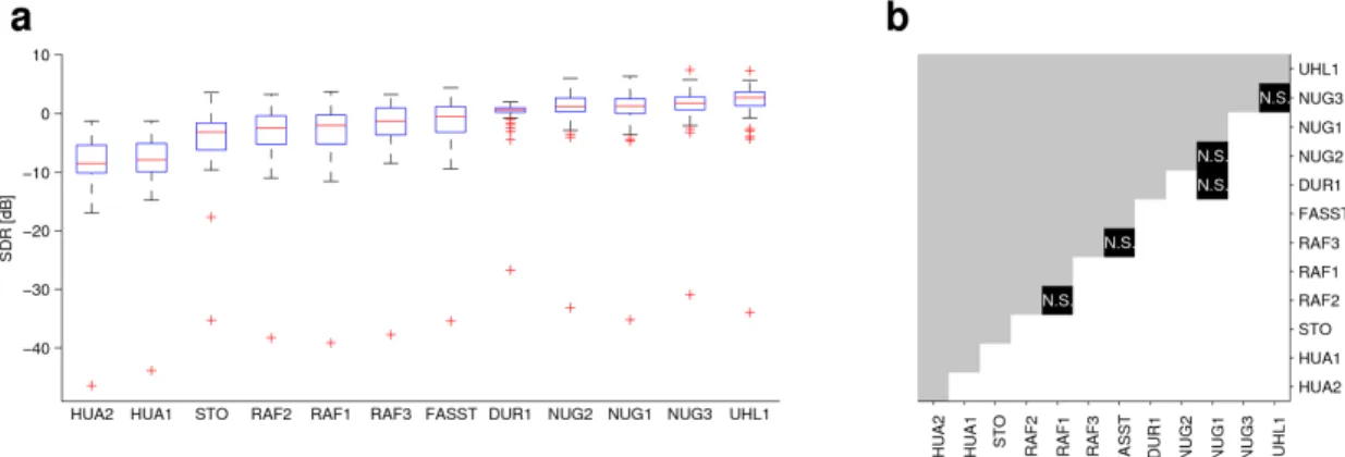
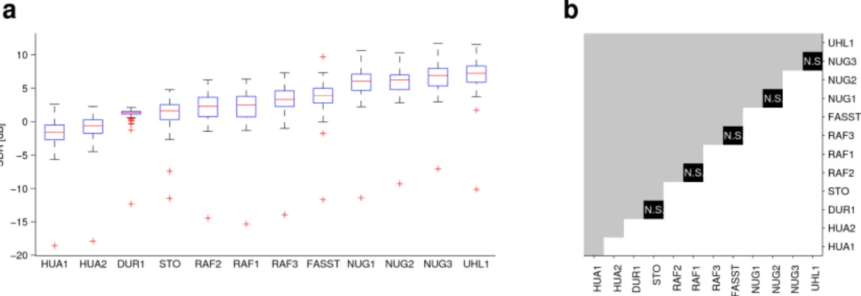
Figures 2a, 3a and 4a show box-plots for each of the models, also with the models ranked in order of median (as in Fig. 1). The boxplots show median (red), the box itself represents inter-quartile range (IQR) and the ‘whiskers’
represent 1.5 x IQR. Outliers (defined as data points outside the 1.5 x IQR ‘whiskers’) are given as red plusses. Fig. 2a shows the boxplots for the vocals. There is a wide spread of SDR but some of the distributions overlap to a large degree. This
generally indicates there may be a lack of evidence for significant differences between adjacent (in ranked order) models. Of particular interest is the fact that the top two models appear very similarly distributed. Fig. 3a shows the boxplots for the accompaniment data. The overall trend is similar to the vocals but the SDR range appears somewhat larger. Fig. 4a shows the boxplots of the overall performance (average across vocal and accompaniment) which supports the same general trends. Main effects (evidence for an effect) of model are seen for the vocal (P < 0.001, χ2 = 443.7, df = 49, Friedman test), for the accompaniment (P < 0.001, χ2 = 354.6, df = 49,
Friedman test) and for the vocal (P < 0.001, χ2 = 253.5, df =
49, Friedman test). Therefore, we proceed to the post-hoc planned contrasts (pair-wise tests).
Fig. 2b plots a significance matrix for the vocal data, also in ranked order (as in the boxplots) which shows the pair-wise comparison of the models via the Wilcoxon signed-rank test. Entries marked ‘N.S.’ indicate ‘Not Significant’ (P > 0.05,
Wilcoxon signed-rank test, two-tailed, Bonferroni corrected) –
all other comparisons are significant (P < 0.05, Wilcoxon
signed-rank test, two-tailed, Bonferroni corrected). This allows
us to select a model comparison of interest (e.g., from the
respective boxplot) and ascertain whether there is evidence for a significant difference. From this matrix we can see that there is no evidence of a significant difference in performance between the two top-ranked models (UHL1, NUG3). Fig. 3b plots the same for the accompaniment data and Fig. 4b plots the same for the average data. Again, in both cases, the same two models (UHL1, NUG3) are top-ranked and again there is no evidence for a significant difference between them.
We also note, in general, that for all the significance matrices there is a consistent trend of some adjacent (by ranks) models not being significantly different. This is not surprising but tends to suggest that the significance of small incremental differences can be difficult to confirm. Furthermore, our results do not find evidence of significant differences between several of the models which are effectively permutations on the same basic architecture. For example, for all three conditions (vocal / accompaniment / average), the pairs RAF1 / RAF2 and NUG1 / NUG2 show no significant inter-pair difference (P > 0.05,
Wilcoxon signed-rank test, two-tailed, Bonferroni corrected).
By contrast, the alternate versions (RAF3 and NUG3 respectively) of the two respective families of model are significantly different to their respective alternate models.
Figure 2. Vocal separation results and significant matrix. a boxplots of the vocal data for each model, ranked in order of median b pair-wise Wilcoxon signed-rank test results. All comparisons blocked in white are significant (P < 0.05, Wilcoxon signed-signed-rank test, two-tailed, Bonferroni corrected) unless annotated with
‘N.S.’. Also ranked in order of median. Note that the upper half of the matrix (in grey) is empty (meaning that the grey area does not convey any information).
Figure 3. Accompaniment separation results and significant matrix. a boxplots of the vocal data for each model, ranked in order of median b pair-wise Wilcoxon signed-rank test results. All comparisons shown in white are significant (P < 0.05, Wilcoxon signed-rank test, two-tailed, Bonferroni corrected) unless annotated
Figure 4. Average (of vocal and accompaniment) separation results and significant matrix. a boxplots of the vocal data for each model, ranked in order of median b pair-wise Wilcoxon signed-rank test results. All comparisons shown in white are significant (P < 0.05, Wilcoxon signed-rank test, two-tailed, Bonferroni
corrected) unless annotated with ‘N.S.’. Also ranked in order of median. Note that the upper half of the matrix (in grey) is empty.
IV. CONCLUSIONS
We have outlined a basic hypothesis-driven procedure for rigorous non-parametric statistical analysis of source separation model results. Our analysis has provided reliable evidence of significant differences in performance between most models. However, we found no evidence of any significant difference between the top two models, both of which are based on Deep Neural Networks (DNN). These two models mainly differ in the way they handle stereo information in music, so it is perhaps not surprising that their results should be similar. Since the dataset considered in this separation evaluation was mostly mono, this result was anticipated and so future work includes application of the same analysis to a stereo dataset.
ACKNOWLEDGMENT
AJRS, GR, EMG and MDP were supported by grants EP/L027119/1 and EP/L027119/2 from the UK Engineering and Physical Sciences Research Council (EPSRC). Data and materials are available from the authors on request.
REFERENCES
[1] P. Smaragdis, C. Fevotte, G. J. Mysore, N. Mohammadiha, M. Hoffman, “Static and dynamic source separation using nonnegative factorizations: A unified view”, Signal Processing Magazine, IEEE, 31(3), 66-75, 2014.
[2] N. Ono, Z Rafii, D. Kitamura, N. Ito, A. Liutkus, “The 2015 Signal Separation Evaluation Campaign.” In Latent Variable Analysis and Signal Separation: 12th International Conference, E. Vincent et al. (Eds.): LVA/ICA 2015, LNCS 9237, pp. 387–395, 2015.
[3] E. Vincent, R. Gribonval, C. Févotte “Performance measurement in blind audio source separation”, IEEE Trans. on Audio, Speech and Language Processing 14:1462-1469, 2006.
[4] J. L. Durrieu, B. David, G. Richard, “A musically motivated mid-level representation for pitch estimation and musical audio source separation”, IEEE J. Sel. Top. Sign. Process. 5(6), 1180–1191, 2011.
[5] P. S. Huang, S.D. Chen, P. Smaragdis, M. Hasegawa-Johnson, “Singing-voice separation from monaural recordings using robust principal component analysis”, In: Proceedings of ICASSP, pp. 57–60, 2012.
[6] A. A. Nugraha, A. Liutkus, E. Vincent, “Multichannel audio source separation with deep neural networks”, Research report RR-8740, Inria, 2015.
[7] Z. Rafii, B. Pardo, “REpeating pattern extraction technique (REPET): a simple method for music/voice separation”, IEEE Trans. ASLP 21(1), 71–82, 2013.
[8] J. Salamon, E. Gomez, “Melody extraction from polyphonic music signals using pitch contour characteristics”, IEEE Trans. ASLP 20(6), 1759–1770, 2012.
[9] F.R. Stoter, S. Bayer, B. Edler, “Unison source separation” In: Proceedings of DAFx, 2014
[10] S. Uhlich, F. Giron, Y. Mitsufuji, “Deep neural network based instrument extraction from music”, In: Proceedings of ICASSP, pp. 2135–2139, 2015.
[11] H. Erdogan, J. R. Hershey, S. Watanabe, J. Le Roux, “Phase-sensitive and recognition-boosted speech separation using deep recurrent neural networks”, In: Proceedings of ICASSP, pp. 708–712, 2015.
[12] A. Ozerov, E. Vincent, F. Bimbot, “A general flexible framework for the handling of prior information in audio source separation”, IEEE Trans. ASLP 20(4), 1118– 1133, 2012.
[13] Y. Salaun, E. Vincent, N. Bertin, N. Souviraa-Labastie, X. Jaureguiberry, D.T. Tran, F. Bimbot, “The flexible audio source separation toolbox version 2.0”, In: Proceedings of ICASSP, 4–9, 2014. [14] T. W. Anderson, D. A. Darling,. “Asymptotic theory of certain
"goodness-of-fit" criteria based on stochastic processes”. Annals of Mathematical Statistics 23: 193–212, 1952.
[15] M. Friedman “The use of ranks to avoid the assumption of normality implicit in the analysis of variance”. Journal of the American Statistical Association (American Statistical Association) 32 (200): 675–701, 1937. [16] M. Friedman, “A correction: The use of ranks to avoid the assumption of normality implicit in the analysis of variance”. Journal of the American Statistical Association (American Statistical Association) 34 (205): 109, 1939.
[17] M. Friedman, “A comparison of alternative tests of significance for the problem of m rankings”. The Annals of Mathematical Statistics 11 (1): 86–92, 1940.
[18] F. Wilcoxon, “Individual comparisons by ranking methods”. Biometrics Bulletin 1 (6): 80–83, 1945.
[19] C. E. Bonferroni, “Teoria statistica delle classi e calcolo delle probabilità”, Pubblicazioni del R Istituto Superiore di Scienze Economiche e Commerciali di Firenze, 1936.