Comparative Spectral Analysis and Correlation Properties of Observed and Simulated Total Column Ozone Records

HAL Id: hal-00850028

https://hal.archives-ouvertes.fr/hal-00850028

HAL is a multi-disciplinary open access

archive for the deposit and dissemination of sci-entific research documents, whether they are pub-lished or not. The documents may come from teaching and research institutions in France or abroad, or from public or private research centers.

L’archive ouverte pluridisciplinaire HAL, est destinée au dépôt et à la diffusion de documents scientifiques de niveau recherche, publiés ou non, émanant des établissements d’enseignement et de recherche français ou étrangers, des laboratoires publics ou privés.

Properties of Observed and Simulated Total Column

Ozone Records

Viktória Homonnai, Imre M. Jánosi, Franck Lefèvre, Marion Marchand

To cite this version:

Viktória Homonnai, Imre M. Jánosi, Franck Lefèvre, Marion Marchand. Comparative Spectral Analy-sis and Correlation Properties of Observed and Simulated Total Column Ozone Records. Atmosphere, MDPI 2013, 4 (2), pp.198-213. �10.3390/atmos4020198�. �hal-00850028�

atmosphere

ISSN 2073-4433 www.mdpi.com/journal/atmosphere Article

Comparative Spectral Analysis and Correlation Properties of

Observed and Simulated Total Column Ozone Records

Vikt´oria Homonnai1_{, Imre M. J´anosi}1,_{*, Franck Lef`evre}2 _{and Marion Marchand}2 1 _{Department of Physics of Complex Systems, E¨otv¨os Lor´and University, P´azm´any P. s. 1/A,}

H-1117 Budapest, Hungary; E-Mail: homonnai.viktoria@gmail.com

2 _{LATMOS-CNRS, Pierre et Marie Curie University, 4 place Jussieu, F-75252 Paris Cedex 05, France;}

E-Mails: franck.lefevre@latmos.ipsl.fr (F.L.); marion.marchand@latmos.ipsl.fr (M.M.) * Author to whom correspondence should be addressed; E-Mail: imre.janosi@ttk.elte.hu;

Tel.: +36-1-372-2878; Fax: +36-1-372-2866.

Received: 24 April 2013; in revised form: 9 May 2013 / Accepted: 11 May 2013 / Published: 14 June 2013

Abstract: We present a statistical analysis of total column ozone records obtained from satellite measurements and from two global climate chemistry models on global scale. Firstly, a spectral weight analysis is performed where the relative strength of semiannual, annual and quasi-biennial oscillations are determined with respect to the integrated power spectra. The comparison reveals some anomalies in the model representations at each spectral component. The tails of the spectra demonstrate that both models underestimate high frequency (daily) ozone variability, which might have a complex origin, since several dynamical processes affect short time changes of the ozone level at a given location. Secondly, detrended fluctuation analysis is exploited to analyze two-point correlations of anomaly time series. Both models reproduce the characteristic geographic dependence of correlation strength over the overlapping area with empirical observations (latitude band between 60◦S and 60◦N). The values of precise correlation exponents are hard to obtain over regions where quasi-biennial oscillations or other strong nonstationarities (ozone hole) are present. In spite of all the numerical difficulties, significant long range correlations are detected for total ozone over all geographic locations.

Keywords: total column ozone; daily time series; global observations; global CCM simulations; spectral properties; correlation properties; quasi-biennial oscillations

1. Introduction

The European project RECONCILE has comprehensively addressed several key questions in the context of polar ozone depletion, with the objective to quantify the rates of some of the most relevant, yet still uncertain physical and chemical processes [1]. The project used an extended toolkit of laboratory experiments, two field missions in the Arctic winter 2009/10 by the research aircraft M55-Geophysica (12 flights of 57 hours), a Match ozonesonde campaign in the winter 2010/11, together with microphysical and chemical transport modeling. One of the main goals was to construct an improved scheme of ozone chemistry for global chemistry climate model (CCM). Since CCMs provide the only tool for long-time projections, their validation and the evaluation of performance are crucial aspects of predicting the time evolution of the stratospheric ozone layer on global scale [2–4].

CCM activities within RECONCILE are carried out with the LMDz-Reprobus model coupling the Reprobus stratospheric chemistry package with the LMDz general circulation model [5–7]. The performance of the model was tested against observations and other CCM models [6,8–11]. The most extended comparison project was the CCM Validation Activity in two runs (CCMVal-1, CCMVal-2), where 18 leading global CCMs are investigated by several observationally-based performance metrics in order to quantify the ability of models in reproducing the dynamics of stratospheric ozone [12]. Various metrics based on climatological mean values, seasonal cycle, variability amplitudes and patterns, etc. are evaluated and compared [12]. Here we focus on the spectral properties and temporal correlations of daily total column ozone (TO) time series on the global scale. Empirical data are obtained from the database compiled and maintained by Bodeker Scientific (http://www.bodekerscientific.com) from satellite and ground based observations [13–15]. Two CCMs are used for the comparison: the LMDz-Reprobus mentioned above, and a quite similar model built up at the Meteorological Research Institute, Tsukuba, Japan [16,17]. The latter is chosen from the CCMVal-2 database because its setup is very close to LMDz-Reprobus (see the next section), however it is among the 6 models from the 18 producing dynamically the quasi-biennial oscillations (QBO) in the equatorial band [12]. This is known to be a difficult task, because it requires a high spatial and temporal resolution to reproduce a realistic spectrum (temporal and spatial) of upward propagating waves in the tropics [16,18,19]. The main question we pose is whether the presence of a QBO in a CCM has a global impact on the correlation properties. A similarly important point is that we intend to produce a reference analysis of two CCMs in order to detect any global effect of an improved ozone chemistry and microphysics to be developed from the findings of the RECONCILE project.

In Section 2, we provide a concise description of empirical and simulated datasets and the methodology of spectral and correlation analysis. Section 3 is devoted to the results of the statistical tests. Global maps of the spectral weight of semiannual, annual and QBO components of the time series are presented and compared for empirical and CCM data. Two-point correlations are investigated by detrended fluctuation analysis (DFA). The signature of long-range correlations (power-law behavior) is detected globally with different strength at different geographic locations. Zonal mean exponents indicate that the reproduction of correlation properties is satisfactory for both models. In Section 4 we discuss the CCM results for the polar regions, where continuous empirical data are missing. Both CCMs

predict an increased “memory” (stronger correlations), which seems to be in accordance with our present knowledge on the role of polar vortices.

2. Data and Methods

Semi-empirical total column ozone time series are obtained from Bodeker Scientific covering the time interval 1979–2011 with daily temporal, and 1.0◦× 1.25◦ _{(lat/lon) spatial resolution. Missing satellite}

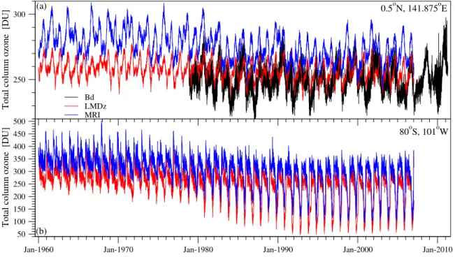
data are complemented by spatial linear interpolation [20,21]. (For this reason, in this work we use the term “empirical data” instead of “measurements”.) Satellite instruments use backscattered solar radiation to infer total column ozone, therefore measurements cannot be made during polar darkness. This fact limits the spatial coverage between 60◦S and 60◦N latitudes. Figure 1(a) illustrates a time series at an equatorial location north to Papua New Guinea (black line). It is easy to see that an annual cycle is missing, instead the variability is dominated by quasi-biennial oscillations.

Figure 1. (a) Empirical and simulated total column ozone (TO) time series for an equatorial location over the Pacific Ocean in Dobson units (DU). Black line belongs to the Bodeker Scientific record (label: Bd), red and blue denote CCM simulations by the LMDz-Reprobus (LMDz) and MRI models; (b) Model time series over the Antarctic (see label). Note the different vertical scales.

250 300

Total column ozone [DU]

Bd LMDz MRI

Jan-1960 Jan-1970 Jan-1980 Jan-1990 Jan-2000 Jan-2010

50 100 150 200 250 300 350 400 450 500

Total column ozone [DU]

0.5oN, 141.875oE

80oS, 101oW (a)

(b)

The two global chemistry climate models selected for comparisons are the LMDz-Reprobus and MRI as mentioned in the Introduction. Both have similar dynamical cores based on the primitive equations with a finite volume horizontal discretization on lat-lon grid [12]. Horizontal resolutions are 2.5◦× 3.75◦

(lat/lon) for the LMDz, and 2.8◦× 2.8◦ _{(T42) for the MRI model, respectively. The vertical grids are}

terrain following hybrid pressure levels in both models with somewhat different resolutions: 50 levels for LMDz, and 68 for MRI. The higher vertical resolution in MRI and weaker horizontal diffusivity in the middle atmosphere than in the troposphere facilitate a dynamical representation of QBO.

The CCMVal-2 project defined a transient run from 1960 (with a 10-year spin-up period) to 2006. Total column ozone (TO) data were obtained at daily temporal resolution by numerically integrating ozone mixing ratios at the individual pressure levels. All forcings in the simulations were taken from observation and included the most important anthropogenic and natural sources (changes in trace gases, solar variability, major volcanic eruptions, QBO, etc.) [12].

The chemistry module Reprobus calculates the chemical evolution of 55 species using 160 gas-phase and 6 heterogeneous reactions, and the sedimentation of polar stratospheric cloud particles is also taken into account. MRI comprises a stratospheric chemistry including 34 long-lived species of 7 families and 15 short-lived species with 79 gas phase reactions and 34 photo-dissociations.

Figure 1 demonstrates a comparison with the satellite data at two “problematic” locations at the equator and at the edge of Antarctica. While QBO is present in the former case (Figure 1(a)), in the latter case (Figure 1(b)) the missing observations make it more difficult to accurately reproduce total column ozone values. Note that the MRI model outputs exhibit a slight overall upward shift of the mean TO levels as it is clearly seen in Figure1.

Next we provide a short overview of the statistical methodology developed in [22], where long range correlations are already detected for ground measurements [23] and satellite TO data (TOMS Nimbus-7) [22]. Here the analysis covers a definitely longer time interval than in [22] and it is extended for global CCM time series.

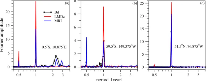
In order the characterize the relative strength of the different components, the spectral weight of a given peak is determined by calculating the area under the peak and normalizing by the total area under the whole spectrum. The estimates are somewhat inaccurate for the wide QBO peaks because the record lengths are limited and the resolution in the Fourier space strongly decays at low frequencies (see Figure2(a)).

Figure 2. Non-normalized power spectra for three different geographic locations (see legends) as a function of period. Note the logarithmic horizontal scales. Black lines with circles belong to the empirical Bodeker Scientific records (label: Bd), red and blue denote CCM simulations by the LMDz-Reprobus (LMDz) and MRI models. (a) Equatorial location (Gabon, Africa); (b) South Pacific Ocean; (c) Qu´ebec, Canada.

0.5 1 2 3 0 5 10 15 20 Fourier amplitude Bd LMDz MRI 0.5 1 2 3 period [year] 0 2 4 6 8 10 0.5 1 2 3 0 5 10 15 20 25 0.5oS, 10.875oE 59.5oS, 149.375oW 51.5oN, 76.875oW (a) (b) (c)

2.1. Spectral Weight Analysis

Power spectra at each grid point are determined by standard Fourier transformation for the three datasets described above. Visual inspection at several locations revealed that three main peaks characterize the TO time series depending on the geographic location: semiannual, annual and QBO components near the equator (see Figure2(a)), a marked semiannual component and missing QBO away from the equator at some places (Figure 2(b)), and a clean annual periodicity in the midlatitude bands, especially on the Northern hemisphere (Figure2(c)).

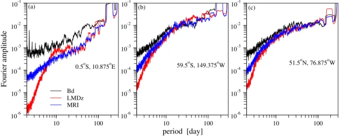
It is quite illuminating to inspect the high frequency tails of the power spectra shown in Figure3for the same geographic locations. A comparison with the empirical data (black lines) reveals that the high frequency variability is underestimated by both CCMs, especially in the equatorial band. (The same is visible already in Figure 1(a)). This might be the consequence of the limited spatial resolution of the global models producing rather smooth meteorological fields, where the representation of subgrid scale processes (e.g., small scale turbulent mixing, breaking internal waves, etc.) is restrained. However, this is a difficult question, because several collateral processes contribute to the short time changes of ozone levels.

Figure 3. The high frequency tails of the spectra in Figure2on double logarithmic scales. Note that the period on the horizontal axes is given in units of day. The same labels, coloring and notations are used. Eleven-point running mean smoothing is applied to suppress high frequency noise. 10 100 10-6 10-5 10-4 10-3 10-2 10-1 Fourier amplitude Bd LMDz MRI 10 100 period [day] 10-6 10-5 10-4 10-3 10-2 10-1 10 100 10-6 10-5 10-4 10-3 10-2 10-1 0.5oS, 10.875oE 59.5oS, 149.375oW 51.5 o N, 76.875oW (a) (b) (c)

Note that a direct quantitative cross-comparison of the empirical and model spectra cannot be easily performed. The standard method of simple normalization does not work because of the different shapes (see Figure3). When a given spectrum exhibits a faster decay at the high frequency tail, normalization gives too large relative weight for the low frequency part. Also matching characteristic peaks (e.g., the annual oscillation) is problematic, because there is no guarantee that a model accurately reproduces a particular component of a signal and fails only at other frequencies.

2.2. Detrended Fluctuation Analysis

The method of detrended fluctuation analysis (DFA) has been developed for quantifying two-point correlations in non-stationary signals, because the autocorrelation function (or power spectrum) can erroneously indicate long range correlations in the absence of strict stationarity. Since DFA has become a standard tool in time series analysis [24–26], we give a very concise summary of the procedure.

Apparent periodic components in a signal spoil the results [27,28], therefore the first step is to obtain an anomaly time series a(t) (t = 1...N ) by computing the difference between an instantaneous TO value and the climatic mean for the given calendar day (obtained from as many years as available). Note that this procedure effectively removes stationary semiannual and annual oscillations from a signal, however it cannot wipe out a global trend or quasi-periodic components such as QBO. DFA regards an anomaly time series as successive increments of a random walk process, thus the next step is the “reconstruction” of the “trajectory” by numerical integration: y(τ ) = Pτ

t=1a(t), τ = 1...N . This signal is divided into

equal segments (windows) of length n, and local trends are determined by a polynomial fit of order p, separately for each segment. The root mean square fluctuation value in a segment is obtained from the variance around the local trend. The DFAp fluctuation function F (n) is calculated as an average of local fluctuation values for a given window size n. This calculation can remove a weak polynomial trend of order p − 1 from the original signal, therefore it provides a more robust tool to quantify correlations than the direct determination of the autocorrelation function or power spectrum.

The presence of overall trends can be tested by comparing the DFAp fluctuation functions at increasing p values. In the case of ozone anomaly time series, we found that the shape of the curves does not change when p > 2, therefore we fixed the order of local polynomial detrending as p = 3. (A needlessly high order slows down the computations and results in higher inaccuracies, because the magnitude of fluctuation functions Fp(n) monotonously decreases with an increasing p.) There is no

methodological consensus around the maximum window size. Various ranges have been used in the literature, and values between nmax = N/10 and N/4 are the most common choices. Detailed tests with

computed model series suggest that even higher nmax values can bear some useful information when

long range correlations are expected [29], therefore we determined the DFA3 fluctuation function for the whole length N of each record. Finally we note that the curves are smoothed by using a sliding window technique, where the window of a given length n is shifted by 1 day along the time axis.

Figure 4 illustrates on double logarithmic scale the DFA3 fluctuation functions (p = 3) for three typical locations: at the equator (Figure4(a)), somewhat away from it (Figure4(b)), and at a midlatitude site (Figure4(c)). Long range correlations are present in the signal when the fluctuation function follows a power law F (n) ∼ nα (straight line in a log-log plot) with exponent values α > 1/2. Clean power law behavior is rarely obtained for empirical data, especially for such complex systems as the atmosphere [22,23,28,30]. The reason is that many different processes of different characteristic time scales affect the instantaneous value of any atmospheric parameter, therefore nonstationarities, various trends, cycles etc. “contaminate” the time series. For example, the apparent kink visible in Figure4(a) for the empirical (black) and MRI (blue) data denoted by a red arrow is a clear consequence of QBO which is not present in the LMDz time series (red). As we mentioned, it is difficult to filter out quasi-periodic components. We tested one possible method, i.e., the Wiener filter for the QBO frequency band, however

we decided not to apply it in the global analysis, because it affects long-range correlations in geographic locations where the QBO is not present at all. Instead, we determined a power law fit in two ranges for each F (n) curve: one is for the whole range of n (dashed lines in Figure4), and the other for a restricted range between 60 days and 15 years (thin solid lines in Figure 4(b,c)). We are fully aware of the fact that the fluctuation functions deviate from a clean power law especially at the terminals of the curves, therefore we use the fitted exponent values as an approximate parameter of correlations. There is no way to visually check thousands of curves in order to determine an optimal fitting range for each of them.

Figure 4. Logarithm of DFA3 fluctuation function log₁₀[F (n)] as a function of logarithmic window size log₁₀n for three different geographic locations (see legends). Black lines belong to the empirical Bodeker Scientific records (label: Bd), red and blue denote CCM simulations by the LMDz-Reprobus (LMDz) and MRI models. (a) Gulf of Guinea, near the equator; (b) Indian Ocean, close to Christmas Island; (c) Guo Dao, Xinjiang, China. Thin dashed lines indicate whole range fits for the LMDz data, thin straight lines in (b) and (c) denote the same for the restricted range (60 days–15 years), see text.

3. Results and Discussion 3.1. Spectral Peak Maps

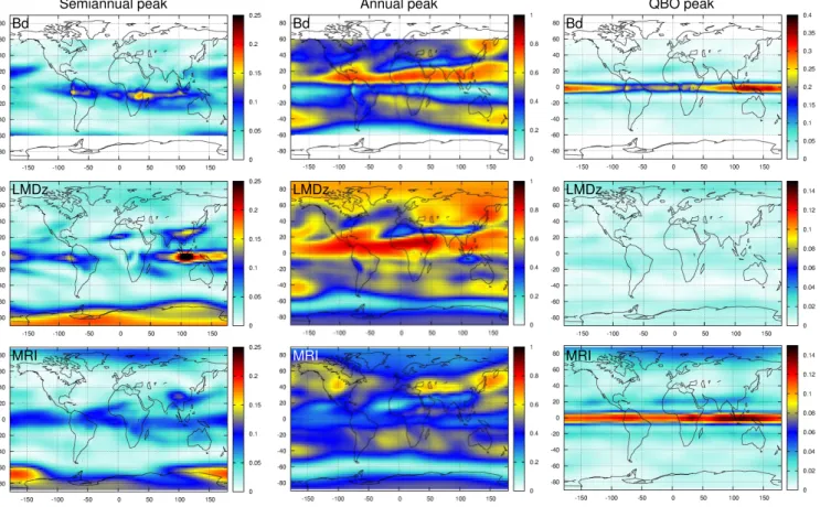
We determined the spectral weights of semiannual, annual and QBO peaks for each power spectrum by the method described in Subsection2.1. Figure5displays the geographic distribution of these weights for the empirical and the two simulated datasets. Semiannual oscillations are better reproduced by the LMDz-Reprobus model around the equator, however the area of strongest spectral weights is shifted towards the East by about 70 degrees (Figure 5, first column). This component is very weak in the MRI signals, however both models indicate its appearance over the Antarctic where empirical data is not available. A remarkable small detail is the visible local maximum over the Tibetan Plateau in both models (albeit weak in MRI again), which is missing from the empirical data.

The annual oscillations are much better represented by the LMDz-Reprobus model (Figure5, second column). The reproduction of the patterns at high latitude values over both hemispheres provides a strong confidence that the annual oscillations are properly simulated over the polar regions. The numerical

values are somewhat higher in the LMDz model than in the empirical data, which is the consequence of too small variability at high frequencies (observed already in Figure3) decreasing the overall area under each spectrum. The annual component is practically missing in the MRI signals around the equator and over the Arctic; even an area of maximal spectral weights appears over North America, which is missing from the empirical data.

Figure 5. Geographic distribution of the spectral peak weights for the empirical Bodeker Scientific records (label: Bd) and CCM simulations by the LMDz-Reprobus (label: LMDz) and MRI models (label: MRI). The columns from left to right display the weights of semiannual, annual and QBO peaks, respectively. Note the different color-scale ranges for the QBO maps.

Semiannual peak Annual peak QBO peak

Bd LMDz Bd LMDz MRI Bd MRI MRI LMDz

The missing QBO component from the LMDz-Reprobus time series is well-known and the reasons are understood [31] (Figure5, third column). The reproduction is more satisfying in the MRI model, however note the different color coded ranges for the empirical and model data: QBO is present but much weaker than in the measured records.

3.2. DFA Exponent Maps

Third order DFA3 fluctuation functions are determined for the three datasets after removing the climatic mean values (see Section 2.2). Although the curves are only approximately straight lines in the log-log plots, we performed power law fits in order to provide a simple characterization on a global

scale. The exponent values are definitely higher than 1/2 everywhere, indicating the presence of long memory processes in the dynamics and chemistry of ozone formation and decay.

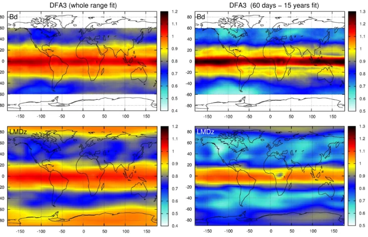
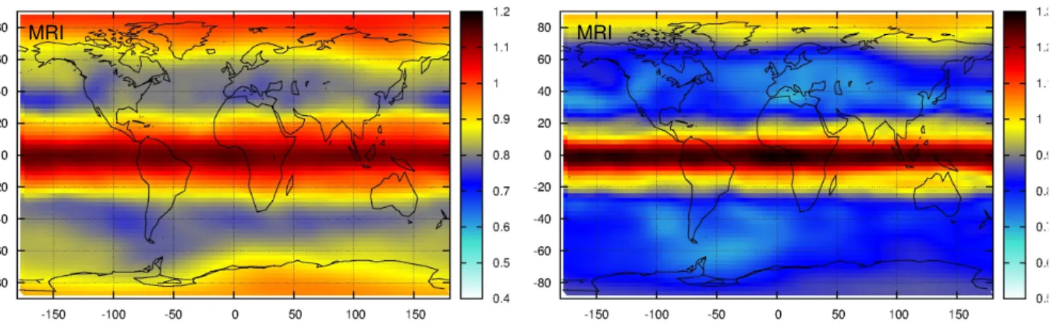
The geographic distribution of the exponent values are color coded and displayed in Figure6. The left column shows the results for whole-range fits, while exponents by restricted-range fits (60 days–15 years) are plotted in the right column. In general, both models seem to properly reproduce the fluctuation functions exhibited by the empirical data. The weak patterns around latitudes −60◦ and 60◦ appearing in the empirical data (Figure 6, top panels) are also present in the maps of model calculations, thus stronger correlations over the polar regions seem to be plausible. This observation is consistent also with our knowledge on stratospheric dynamics: meridional mixing is weaker across the walls of polar vortices, thus longer “memory” is expected in the internal regions. The stronger correlations (higher exponent values) around the equator were found already in [22] for shorter satellite records. The most probable reason for the weaker correlations in the midlatitude bands is the two-way coupling between the troposphere and stratosphere [32], e.g., the stronger dynamic activity in the troposphere in these geographic ranges excite more energetic internal gravity waves entering the stratosphere and inducing more intense mixing.

Figure 6. Geographic distribution of the DFA3 exponent values for the empirical Bodeker Scientific records (label: Bd) and CCM simulations by the LMDz-Reprobus (label: LMDz) and MRI models (label: MRI). The left column displays fitted values for the whole range of available data, the right column shows the results for the restricted range fits from 60 days to 15 years (from 1.78 to 3.74 on the log10axis), see Figure4.

DFA3 (whole range fit) DFA3 (60 days − 15 years fit)

LMDz LMDz

MRI MRI

Atmosphere2013, 4 207

Figure 6. Cont.

LMDz LMDz

MRI MRI

Figure7displays the zonal mean values of the exponents as a function of geographic latitudes. The model reproductions are satisfying, the main features (weaker correlations in the midlatitude bands) are present in both CCMs. The comparison of Figure6(a) (whole range fits) and Figure6(b) (restricted range fits) reveals the effect of QBO kinks present in the empirical and MRI model fluctuation functions (see Figure4(a), red arrow): the apparent exponent values are systematically higher than in the case of whole range fits. Since the LMDz model does not have QBO, such effect is missing (red curves in Figure 6). The changes of exponent values away from the equator are due to the tail effects, both for small and large segment sizes n.

Figure 7. Zonal mean values of the DFA3 exponents for the empirical Bodeker Scientific records (label: Bd) and CCM simulations by the LMDz-Reprobus (label: LMDz) and MRI models (label: MRI) as a function of geographic latitude. (a) Fitted values for the whole range of available data; and (b) restricted range fits from 60 days to 15 years (from 1.78 to 3.74 on the log10axis), see Figure4. Error bars represent the variability of exponent values

along a circle of latitude.

-90° -60° -30° 0° 30° 60° 90° latitude 0.5 0.6 0.7 0.8 0.9 1.0 1.1 1.2 1.3 1.4 < α > -90° -60° -30° 0° 30° 60° 90° latitude 0.5 0.6 0.7 0.8 0.9 1.0 1.1 1.2 1.3 1.4 < α > Bd LMDz MRI (a) (b)

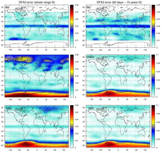
Deviations from a pure power law behavior are also detected by the numerical values of the standard error of fitted slope coefficient. This quantity is color coded and plotted in Figure 8 both for the whole and restricted range fits. The most prominent feature for the empirical data (Figure 8(top)) is a band of somewhat higher fitting error around the equator. This is explained by the presence of QBO, which cannot be easily filtered out, and it is manifested as a marked kink on DFA3 fluctuation curves

(cf. Figure 4(a)). This band is much weaker for the MRI simulations (Figure 8(bottom)), which is consistent with the results of spectral analysis ((Figure5(bottom right)) indicating a QBO component of a suppressed amplitude compared with empirical data.

Figure 8. Geographic distribution of the standard fitting error of DFA3 exponent values for the empirical Bodeker Scientific records (label: Bd) and CCM simulations by the LMDz-Reprobus (label: LMDz) and MRI models (label: MRI). The left column displays fitted values for the whole range of available data, the right column shows the results for the restricted range fits from 60 days to 15 years (from 1.78 to 3.74 on the log10 axis), see

Figure4. Note the different color scales at the two columns.

DFA3 error (whole range fit) DFA3 error (60 days − 15 years fit)

MRI MRI

LMDz

LMDz

Bd Bd

Anomalously strong fitting errors appear above the Antarctic for both sets of CCM simulations (Figure 8middle and bottom). Note that a precursor pattern is also visible in the empirical data close to −60◦ (lat), between −150◦ and −50◦(long), which is definitely enhanced toward the south pole. An explanation is given in Figure9, where DFA3 fluctuation functions and power spectra are plotted for two locations over the Antarctic. The main problem is caused by the extreme nonstationary behavior of the

ozone time series in this region associated with the ozone hole [33,34]. Figure1(b) clearly demonstrates a strong overall trend, which can be wiped out by a polynomial fit without any difficulty. However, besides the drop of mean ozone levels, the amplitude of the annual cycle is almost doubled since the 1980s, and this kind of variability change cannot be filtered out by computing climatic mean values. Figure9(c) shows that a residual annual (and even semiannual) periodicity remains in the signal, which leads to the appearance of the kinks in Figure9(a,b).

Figure 9. (a) and (b): Logarithm of DFA3 fluctuation function log₁₀[F (n)] as a function of logarithmic window size log₁₀n for two different geographic locations (see legends) over the Antarctic. Red and blue denote CCM simulations by the LMDz-Reprobus (LMDz) and MRI models, empirical data are not available; Red arrow on (b) indicates the characteristic kink appearing everywhere for locations over the Antarctic; (c) Power density spectra for the total column ozone anomaly records (annual cycle removed) simulated by the LMDz (red) and MRI (blue) models over an Antarctic location (see legend).

1 2 3 4 log 10(n) 1 2 3 4 log 10 [F(n)] LMDz MRI 1 2 3 4 log 10(n) 1 2 3 4 1 10 period [year] 0 2 4 6 8 10 Fourier amplitude 80oS, 101oW 77oS, 67.5oW 77oS, 67.5oW (a) (b) (c)

Besides [22] and the present work, the most comprehensive analyses of total ozone correlations were performed in [35,36] on global scale. In the latter studies, monthly mean data were evaluated at rather low spatial resolution (5◦× 10◦_{, lat-long). The period of 29 years provided short time series of}

length of 348 points. Each time series was fitted by a combined statistical model of 21 free parameters consisting of the mean, the seasonal cycle, the QBO component, the solar cycle, a long-term trend, and residuals (noise). Apart from side effects of possible over-fitting, e.g., Figure 3 in [36] demonstrates fully inconsistent results depending on the method of estimating correlation exponents. The detected behavior changes from uncorrelated noise to extremely strong long range correlations at the same geographic latitude. We also found that numerical values are sensitive to the way of filtering and range of fitting (see Figure7), however our results reflect consistency both for the three datasets and in a geographic sense: it is quite improbable that correlation properties change hectically from one latitude band to another. 4. Conclusions

• Both the LMDz and MRI models provide an adequate reproduction of empirical data in the period of comparison (see Figure 1), however the latter seems to slightly overestimate total column ozone values.

• Spectral analysis reveals that both models underestimate high frequency (daily) variability (see Figure 3), MRI performs better from this point of view. Such deficiency might have a rather complex origin, because several dynamical processes (advection, diffusion and mixing) contribute to short time fluctuations.

• Spectral weight analysis indicates some anomalies in the dynamical core of both CCMs. The geographic locations of semiannual oscillations are shifted in the models. MRI is known to reproduce the QBO mode along the equator (albeit it is definitely weaker than in the empirical records), however it underperforms with respect of the annual component.

• The presence of quasi-biennial oscillations decreases the accuracy of DFA analysis (see Figure 4(a)). Band pass Fourier filtering can remove such spectral component (see [22]), however one should be careful, because the DFA method is based on residual (anomaly) analysis. Specifically, the standard Wiener filtering consists of two steps: firstly, the Fourier transform of a given time series is produced and the amplitudes are set to be zero or to some assumed (practically interpolated) base line values in the required frequency ranges, and secondly, an inverse Fourier transform produces the filtered time series. When this method is applied on a global scale, obviously the filtered components disappear everywhere, also from signals where QBO oscillations are not present. Care should be taken especially when the target is to detect long range correlations, because such procedure might distort the original properties of the time series. Too strong filtering can yield (geographically) inconsistent results as probably demonstrated in [35,36].

Note that the low model values of high frequency variabilities are reflected by the fact that the initial parts of fluctuation functions remain systematically below the curve for empirical data (Figure4).

• The DFA3 fluctuation functions are adequately reproduced by both CCMs (see Figures6and7). We do not claim that the curves represent pure power law behavior (see Figure4); still the overall trends are close to linear on log-log scale, indicating the presence of long range correlations. (The appearance of clean power laws is not even expected, because many processes of various characteristic time scales contribute to the instantaneous value of any atmospheric variable at a given location.)

• Since the reproduction of correlation properties in the models is quite satisfactory in the overlapping geographic latitude band between −60◦ and 60◦, we can have a strong confidence in the prediction of both models that correlations are stronger over both polar regions. This observations is also supported by considering the role of polar vortices in the meridional transport processes.

• Classical methods of time series analysis have a limited applicability over the polar regions, especially over the Antarctic. Such strong nonstationary signals as represented by the total ozone level during the decades of ozone hole make any residual (anomaly) analysis very difficult. Standard methods to remove semiannual and annual oscillations fail when the amplitudes

change strongly (see Figure 9), however an over-filtering might yield information loss about correlation properties.

Acknowledgements

The present work is supported by the Hungarian Science Foundation under the grant number OTKA NK100296, and by the European Commission under the grant number RECONCILE-226365-FP7-ENV-2008-1.

Conflict of Interest

The authors declare no conflict of interest. References

1. Von Hobe, M.; Bekki, S.; Borrmann, S.; Cairo, F.; D’Amato, F.; Di Donfrancesco, G.; D¨onbrack, A.; Ebersoldt, A.; Ebert, M.; Emde, C.; et al. Reconciliation of essential process parameters for an enhanced predictability of Arctic stratospheric ozone loss and its climate interactions. Atmos. Chem. Phys. Discuss. 2012, 12, 30661–30754.

2. Butchart, N.A.; Charlton-Perez, A.J.; Cionni, I.; Hardiman, S.C.; Haynes, P.H.; Kr¨uer, K.; Kushner, P.J.; Newman, P.A.; Osprey, S.M.; Perlwitz, J.; et al. Multimodel climate and variability of the stratosphere. J. Geophys. Res. 2011, 116, D05102, doi:10.1029/2010JD014995.

3. Douglass, A.R.; Stolarski, R.S.; Strahan, S.E.; Oman, L.D. Understanding differences in upper stratospheric ozone response to changes in chlorine and temperature as computed using CCMVal-2 models. J. Geophys. Res. 2012, 117, D16306, doi:10.1029/2012JD017483.

4. Gettelman, A.; Eyring, V.; Fischer, C.; Shiona, H.; Cionni, I.; Neish, M.; Morgenstern, O.; Wood, S.W.; Li, Z. A community diagnostic tool for chemistry climate model validation. Geosci. Model Dev. 2012, 5, 1061–1073.

5. Hourdin, F.; Musat, I.; Bony, S.; Braconnot, P.; Codron, F.; Dufresne, J.-L.; Fairhead, L.; Filiberti, M.-A.; Friedlingstein, P.; Grandpeix, J.-Y.; et al. The LMDz4 general circulation model: Climate performance and sensitivity to parametrized physics with emphasis on tropical convection. Clim. Dyn. 2006, 27, 787–813.

6. Jourdain, L.; Bekki, S.; Lott, F.; Lef`evre, F. The coupled chemistry climate model LMDz-REPROBUS: Description and evaluation of a transient simulation of the period 1980–1999. Ann. Geophys. 2008, 26, 1391–1413.

7. Marchand, M.; Keckhut, P.; Lefebvre, S.; Claud, C.C.D.; Hauchecorne, A.; Lef`evre, F.; Lefebvre, M.-P.; Jumelet, J.; Lott, F.; Hourdin, F.; et al. Dynamical amplification of the stratospheric solar response simulated with the Chemistry-Climate model LMDz-Reprobus. J. Atmos. Solar-Terrest. Phys. 2012, 75–76, 147–160.

8. Austin, J.; Scinocca. J.; Plummer, D.; Oman, L.; Waugh, D.; Akiyoshi, H.; Bekki, S.; Braesicke, P.; Butchart, N.; Chipperfield, M.; et al. The decline and recovery of total column ozone using a multi-model time series analysis. J. Geophys. Res. 2010, 115, D00M10, doi:10.1029/2010JD013857.

9. Gettelman, A.; Hegglin, M.I.; Son, S.-W.; Kim, J.; Fujiwara, M.; Birner, T.; Kremser, S.; Rex, M.; A˜nel, J.A.; Akiyoshi, H.; et al. Multimodel assessment of the upper troposphere and lower stratosphere: Tropics and global trends. J. Geophys. Res. 2010, 115, D00M08, doi:10.1029/2009JD013638.

10. Hegglin, M.I.; Gettelman, A.; Hoor, P.; Krichevsky, R.; Manney, G.L.; Pan, L.L.; Son, S.W.; Stiller, G.; Tilmes, S.; Walkeret, K.A.; et al. Multimodel assessment of the upper troposphere and lower stratosphere: Extratropics. J. Geophys. Res. 2010, 115, D00M09, doi:10.1029/2010JD013884. 11. Hourdin, F.; Foujols, M.-A.; Codron, F.; Guemas, V.; Dufresne, J.-L.; Bony, S.; Denvil, S.;

Guez, L.; Lott, F.; Ghattas, J.; et al. Impact of the LMDZ atmospheric grid configuration on the climate and sensitivity of the IPSL-CM5A coupled model. Clim. Dyn. 2012, doi:10.1007/s00382-012-1411-3.

12. SPARC CCMVal. SPARC Report on the Evaluation of Chemistry-Climate Models; Eyring, V., Shepherd, T.G., Waugh, D.W., Eds.; SPARC Report No. 5; WCRP-132; WMO/TD-No. 1526; 2010. Available online: http://www.sparc-climate.org/publications/ (accessed on 15 June 2010). 13. Bodeker, G.E.; Shiona, H.; Eskes, H. Indicators of Antarctic ozone depletion. Atmos. Chem. Phys.

2005, 5, 2603–2615.

14. M¨uller, R.; Grooß, J.-U.; Lemmen, C.; Heinze, D.; Dameris, M.; Bodeker, G.E. Simple measures of ozone depletion in the polar stratosphere. Atmos. Chem. Phys. 2008, 8, 251–264.

15. Struthers, H.; Bodeker, G.E.; Austin, J.; Bekki, S.; Cionni, I.; Dameris, M.; Giorgetta, M.A.; Grewe, V.; Lef`evre, F.; Lott, F.; et al. The simulation of the Antarctic ozone hole by chemistry-climate models. Atmos. Chem. Phys. 2009, 9, 6363–6376.

16. Shibata, K.; Deushi, M.; Sekiyama, T.T.; Yoshimura, H. Development of an MRI chemical transport model for the study of stratospheric chemistry. Papers Meteorol. Geophys. 2005, 55, 75–119. 17. Shibata, K.; Deushi, M. Long-term variations and trends in the simulation of the middle atmosphere

1980–2004 by the chemistry-climate model of the Meteorological Research Institute. Ann. Geophys. 2010, 26, 1299–1326.

18. Giorgetta, M.A.; Manzini, E.; Roeckner, E. Forcing of the quasi-biennial oscillation from a broad spectrum of atmospheric waves. Geophys. Res. Lett. 2002, 29, 86:1—86:4.

19. Giorgetta, M.A.; Manzini, E.; Roeckner, E.; Esch, M.; Bengtsson, L. Climatology and forcing of the Quasi-Biennial Oscillation in the MAECHAM5 model. J. Clim. 2006, 19, 3882–3901.

20. Bodeker, G.E.; Scott, J.C.; Kreher, K.; McKenzie, R.L. Global ozone trends in potential vorticity coordinates using TOMS and GOME intercompared against the Dobson network: 1978–1998. J. Geophys. Res. 2001, 106, 23029–23042.

21. Bodeker, G.E.; Connor, B.J.; Liley, J.B.; Matthews, W.A. The global mass of ozone: 1978–1998. Geophys. Res. Lett. 2001, 28, 2819–2822.

22. Kiss, P.; M¨uller, R.; J´anosi, I.M. Long-range correlations of extrapolar total ozone are determined by the global atmospheric circulation. Nonlin. Proc. Geophys. 2007, 14, 435–442.

23. J´anosi, I.M.; M¨uller, R. Empirical mode decomposition and correlation properties of long daily ozone records. Phys. Rev. E 2005, 71, 056126, doi:10.1103/PhysRevE.71.056126.

24. Kantz, H.; Schreiber, T. Nonlinear Time Series Analysis; Cambridge University Press: Cambridge, UK, 2004.

25. Derby, N.B. Assessing the Detrended Fluctuation Analysis Method of Estimating the Hurst Coefficient; University of Washington: Seattle, WA, USA, 2004.

26. Lowen, S.B.; Teich, M.C. Fractal-Based Point Processes; John Wiley & Sons: Hoboken, NJ, USA, 2005.

27. Hu, K.; Ivanov, P.Ch.; Chen, Z.; Carpena, P.; Stanley, H.E. Effect of trends on detrended fluctuation analysis. Phys. Rev. E 2001, 64, 011114, doi:10.1103/PhysRevE.64.011114.

28. Kir´aly, A.; J´anosi, I.M. Stochastic modeling of daily temperature fluctuations. Phys. Rev. E 2002, 65, 051102, doi:10.1103/PhysRevE.65.051102.

29. Xu, L.; Ivanov, P.Ch.; Hu, K.; Chen, Z.; Carbone, A.; Stanley, H.E. Quantifying signals with power-law correlations: A comparative study of detrended fluctuation analysis and detrended moving average techniques. Phys. Rev. E 2005, 71, 051101, doi:10.1103/PhysRevE.71.051101. 30. Pattanty´us- ´Abrah´am, M.; Kir´aly, A.; J´anosi, I.M. Nonuniversal atmospheric persistence: Different

scaling of daily minimum and maximum temperatures. Phys. Rev. E 2004, 69, 021110, doi:10.1103/PhysRevE.69.021110.

31. Khosrawi, F.; M¨uller, R.; Urban, J.; Proffitt, M.H.; Stiller, G.; Kiefer, M.; Lossow, S.; Kinnison, D.; Olschewski, F.; Riese, M.; Murtagh, D. Assessment of the interannual variability and impact of the QBO and upwelling on tracer-tracer distributions of N2O and O3in the tropical lower stratosphere.

Atmos. Chem. Phys. 2013, 13, 3619–3641.

32. Gerber, E.P.; Butler, A.; Calvo Fernandez, N.; Charlton-Perez, A.; Giorgetta, M.; Manzini, E.; Perlwitz, J.; Polvani, L.M.; Sassi, F.; Scaife, A.A.; et al. Assessing and understanding the impact of stratospheric dynamics and variability on the Earth system. Bull. Am. Meteor. Soc. 2012, 93, 845–859.

33. Farman, J.C.; Gardiner, B.G.; Shanklin, J.D. Large losses of total ozone in Antarctica reveal seasonal ClOx/NOx interaction. Nature 1985, 315, 207–210.

34. Solomon, S. Stratospheric ozone depletion: A review of concepts and history. Rev. Geophys. 1999, 37, 275–316.

35. Vyushin, D.I.; Fioletov, V.E.; Shepherd, T.G. Impact of long-range correlations on trend detection in total ozone. J. Geophys. Res. 2007, 112, D14307, doi:10.1029/2006JD008168.

36. Vyushin, D.I.; Shepherd, T.G.; Fioletov, V.E. On the statistical modeling of persistence in total ozone anomalies. J. Geophys. Res. 2010, 115, D16306, doi:10.1029/2009JD013105.

c

2013 by the authors; licensee MDPI, Basel, Switzerland. This article is an open access article distributed under the terms and conditions of the Creative Commons Attribution license (http://creativecommons.org/licenses/by/3.0/).