Fluxes of carbon dioxide at Thetford Forest

HAL Id: hal-00305608

https://hal.archives-ouvertes.fr/hal-00305608

HAL is a multi-disciplinary open access archive for the deposit and dissemination of sci-entific research documents, whether they are pub-lished or not. The documents may come from teaching and research institutions in France or abroad, or from public or private research centers.

L’archive ouverte pluridisciplinaire HAL, est destinée au dépôt et à la diffusion de documents scientifiques de niveau recherche, publiés ou non, émanant des établissements d’enseignement et de recherche français ou étrangers, des laboratoires publics ou privés.

To cite this version:

P. G. Jarvis, J. B. Stewart, P. Meir. Fluxes of carbon dioxide at Thetford Forest. Hydrology and Earth System Sciences Discussions, European Geosciences Union, 2007, 11 (1), pp.245-255. �hal-00305608�

© Author(s) 2007. This work is licensed under a Creative Commons License.

Fluxes of carbon dioxide at Thetford Forest

Paul G. Jarvis

_{, John B. Stewart}

_{and Patrick Meir}

1_{School of GeoSciences, The Crew Building, The King’s Buildings, University of Edinburgh, Edinburgh EH9 3JN, UK} 2_{Department of Geography, University of Southampton, Highfield, Southampton SO17 1BJ, UK}

Email for corresponding author: margaretsjarvis@aol.com

Abstract

The Thetford Project (1968–1976) was a keystone project for the newly established Institute of Hydrology. Its primary objective was to elucidate the processes underlying evaporation of transpired water and intercepted rainfall from plantation forest, so as to explain hydrological observations that more water was apparently returned to the atmosphere from plantations than from grassland and heathland. The primary approach was to determine the fluxes of water vapour from a stand of Scots pine, situated within a larger area of plantations of Scots and Corsican pine, in Thetford Forest, East Anglia, UK, using the Bowen ratio approach. In 1976, advantage was taken of the methodology developed to add measurement of profiles of carbon dioxide concentration so as to enable the fluxes of CO2 also to be calculated. A team from

Aberdeen and Edinburgh Universities collected 914 hours of 8-point CO2 concentration profiles, largely between dawn and dusk, on days

from March to October, and the data from an ‘elite’ data set of 710 hours have been analysed. In conditions of moderate temperature (< 25o_C)

and specific humidity deficit (<15 g kg–1 _{with high solar irradiance (>500 W m}-2)_{, CO}

2 uptake reached relatively high rates for pine of up to

20 mmol m–2_s–1 _{in the middle of the day. This rate of CO}

2 uptake is higher than has been recently found for four Scots pine forests in

continental Europe during July 1997. However, the year of 1976 was exceptionally hot and dry, with air temperatures reaching 30 o_{C and the}

water deficit in the top 3 m of soil at the site of 152 mm by August. Air temperatures of over 25o_{C led to large specific humidity deficits,}

approaching 20 g kg–1_{, and associated severe reductions in CO}

2 uptake, as well as in evaporation. However, when specific humidity deficits

dropped below c. 15 g kg–1 _{on succeeding days, generally as a result of lower air temperatures rather than lower solar irradiance, there was}

rapid recovery in both uptake and evaporation, thus indicating that the large soil water deficit was not the main cause of the reductions in the CO2 and water fluxes. Based on earlier analysis of evaporation data on completely dry days, the concurrent reductions in CO2 flux and

evaporation are largely attributable to decrease in canopy stomatal conductance. The air temperature, specific humidity deficit, and soil water deficit in 1976 were exceptional and similar conditions have most likely not been experienced again until 2003. We conclude that the information gained at Thetford in 1976 on the response of the pine forest ecosystem to such weather, may provide a good guide to the response of English pine forests to the projected climate change over the next 25 years.

Keywords: Scots pine, 1976 drought, CO2 flux, Thetford Project

Introduction

In the 1950s, evidence was produced at the catchment scale in the UK showing that runoff from forested areas was less than from grassland. During this same period there was major planting of forests on upland areas, many of which were the catchments of water supply reservoirs. The then government set up the Hydrological Research Unit (later renamed the Institute of Hydrology, and now known as the Centre for Ecology and Hydrology, Wallingford) to investigate the effect of land-use changes on water resources. Studies by Howard Penman at Rothamsted Research Station, led him to postulate that all vegetation should behave like

green blotting paper, so there should be no major differences between the evaporation from short vegetation and that from forests, unless there were large soil moisture deficits. At that time the experimental results of Rutter had shown that the rates of transpiration and of evaporation of intercepted rainfall were very different, implying that total evaporation from forests would be larger than from grass. Thus there was a major disagreement between the theoretical studies of Penman and the experimental results of Rutter. The latter’s results were criticised, however, because they were based on small scale measurements within a forest canopy. Initially, the Hydrological Research Unit proposed to instrument

paired forested and grassed catchments to investigate any hydrological differences between these land uses, and indeed they did so.

However, catchment studies alone would be unable to determine the components of evaporation, which would be required to settle the opposing views of Penman and Rutter. This could only be done by a process study, so in 1967 a major study, which became known as the Thetford Project, was initiated in Thetford Forest, East Anglia, UK. By using micrometeorological techniques the two main components of the evaporation — transpiration and evaporation of intercepted rainfall — could be measured from an extensive area of generally homogeneous forest growing in an area with very little topographical variation (Gash and Stewart, 1975). The micrometeorological technique used to measure the evaporation components was based on the Bowen ratio energy budget with a thermometer interchange system (McNeil and Shuttleworth, 1975) to measure the very small temperature and humidity gradients that occur over aerodynamically rough forest canopies. The use of high tech (and expensive) Hewlett Packard Quartz Crystal™ thermometers to determine the wet and dry bulb temperatures overcame the problems of electrical resistances resulting from long leads and connectors, which had bedevilled the use of thermocouple and resistance thermometers used in earlier studies over forests.

The Thetford Project was also innovative at the time in that it used a computer housed in a caravan in the forest to control all the data acquisition and convert the raw data into suitable averages in engineering units in real time. By today’s standards the computer’s memory was very small indeed — only 32 kbytes — but physically it was very large, 1.5 m tall and weighing about 50 kg. The programming for the system had to be rigorously optimised for efficiency (Sylvia Oliver, personal communication).

To exploit the technological investment in the Thetford Project, a team from Aberdeen and Edinburgh Universities that had previously been making measurements of stomatal resistances and carbon dioxide fluxes in a Sitka spruce plantation in Fetteresso Forest, part of the Forest of Mearns, in Kincardinshire, joined the project for the final two years (1975–1976). The objectives were to add measurements of CO2 fluxes, using both porometer (Beadle et al., 1985a,b,c)

and micrometeorological techniques (Jarvis, 1994) to the Thetford Project. At the time, the main interest in the CO2

flux was in its net uptake for tree growth. Today, the main interest lies in the net removals of CO2 from the atmosphere

by forests, from the perspective of climate change. The 1976 summer in the south of England was one of the hottest and driest in the 20th Century, prior to the sequence of hot years in the 1990s. Thus these data on CO2 exchange provide an

indication of how native pine forests may be expected to respond to the projected rise in atmospheric temperature in the near future.

The extensive and flat Thetford Forest site had a major advantage for measurements of fluxes compared to the hilly Fetteresso site, where advection was more likely to be a problem. Furthermore, the more continental climate of East Anglia contrasted markedly with the cool, humid, oceanic climate of Kincardinshire. Thus the comparison between Sitka spruce and Scots pine would also be of interest and would lead to improved understanding of the processes controlling the fluxes of CO2 fluxes from forests. Before

this publication, a comparison between CO2 fluxes of Sitka

spruce and Scots pine growing in the UK had been made for just one day (Jarvis, 1981).

The research site

The site is near the centre of one of the three main blocks of Thetford Forest in the Breckland of East Anglia, 2 km SW of the village of Brandon, Norfolk (FC Compartment H122, latitude 52o _{25’ N, longitude 0}o _{40’ E, altitude 46 m). The}

area had previously been used for rough grazing but was planted in 1931 with native Scots pine (Pinus sylvestris L.) of Strathspey (Invernessshire/Morayshire) provenance and Corsican pine Pinus nigra var. maritima (Ait.) Melv., at a spacing of 1.4 × 1.4 m on parallel ploughed ridges. The instrument towers were situated in a stand of Scots pine; the surrounding area of stands of Scots and Corsican pine extended in most directions further than two kilometres. By 1976, the Scots pine stand had reached a height of 16.5 m and had been thinned several times, by both man and wind-throw, to a density of 619 stems per hectare. The average height of the stand was 16.5 m, dbh 226 cm, basal area 24.9 m2 _ha–1_{, and volume (over bark ) 212 m}3 _ha–1 _{(Beadle et al.,}

1982).

The live crowns of the trees extended from c. 9 m to tree top. At the beginning of the year, the leaf area index (LAI) was c. 1.9 declining to c. 1.7 prior to bud-burst, which commenced in mid-June, building up to a maximum LAI on 12th August of 2.73 m2 _m–2 _{of which 36% was made up}

of new, current-year needles (Beadle et al., 1982). Beneath the trees, bracken (Pteridium aquilinum (L.) Kuhn) grew up each summer to reach an average height of 1 m and gave a nearly complete ground cover, interspersed with small grassy patches. In 1976, the bracken LAI increased from zero in May to c. 1.1 at the end of June, remained steady from June to mid-September, apart from a short–lived decline to c. 0.6 in mid-August, before finally declining to c. 0.6 in mid-October, and zero again in November (Roberts et al., 1980). The bracken thus contributed appreciably to

the functional ‘leaf’ area through the productive part of the year.

The soil is part of the Worlington series and overlies deposits of c. 0.5 to1.5 m of chalk–sand drift. The surface horizon consists of c. 10 cm of litter and humus overlying variable depths of sand of aeolian origin (Corbett, 1973; Roberts, 1976). The topography is flat or gently undulating.

The weather of 1976

The long-term average annual maximum and minimum temperatures (1961–1990) for central East Anglia are 13.2 and 5.5o_{C, respectively; with June and July average maxima}

of 19.1 and 21.0o_{C, respectively, and average annual}

precipitation of 550 mm. The summers of 1975 and 1976 were, however, far from average. For the period following the dry summer of 1975, the rainfall over England was generally less than half the long term average. The exceptionally dry months of 1975 continued into 1976, when there was serious drought in the region through to the end of August. Birch trees were seen to be dying along roadsides; there were widespread bans on the use of hose-pipes, and water was available only at stand-pipes in several towns and villages. The drought was finally broken in the autumn with September–December having much above average rainfall, so that by the end of 1976 the annual rainfall over England was again close to the long-term average. Such extreme conditions have not reccurred at Thetford Forest until 2003 when there were widespread reductions in forest productivity in Europe (Ciais et al., 2005).

For Thetford Forest the summer of 1976 was also exceptional by comparison with England as a whole, because of the longest period in the last 100 years — in excess of 16 days — with maximum temperatures above 30°C, together with rainfall during the summer months June–August 88 mm below average. The water deficit of the soil profile increased almost linearly from zero in February to c. 152 mm in the upper 3 m of the profile by August, with half this deficit in the topmost metre where the soil is predominantly sand (Cooper, 1980).

On several of the measurement days in June and July, air temperatures above the forest canopy exceeded 28o_{C, the}

corresponding specific humidity deficit (D) approached 20 g kg–1_{, and the canopy surface temperature reached 30}o_C

(Table 1).

Methodology

THEORY

The CO2 flux has been derived using the sensible heat flux

as a tracer (Denmead and McIlroy, 1971). Over a defined height interval, the flux of CO2 is the product of the

concentration difference (DC, parts per million by volume, ppmv, mmol mol–1_{) across the height interval and the}

corresponding aerodynamic conductance, ga, as follows:

Fc = ga(DC)rc, (1)

where rc is the density of CO2.

The aerodynamic conductance for sensible heat flux is given by:

Table 1. Daytime fluxes of CO2 (Fc, mmol m–2 s–1) and water vapour

(E, g m–2 _s–1_{) on the 8}th _{and 9}th _{June and the 7}th _{and 8}th _{July, in} association with solar radiation (Q, mmol m–2 _s–1_{), air temperature} (T, ºC) and specific humidity deficit (D, g kg–1_{), to illustrate the} marked effects of extreme atmospheric conditions on such days. Negative signs indicate removal of CO2 from the atmosphere, i.e. uptake by photosynthesis in trees and bracken; positive signs indicate emissions of CO2 to the atmosphere, i.e. loss by respiration from plant and soil.

Date Hour T D Q Fc E 8 June 10 25.10 9.63 771 –13.39 0.06 8 June 11 26.34 14.44 819 –4.41 0.04 8 June 12 26.78 15.58 825 –7.81 0.06 8 June 13 27.00 15.72 771 –3.54 0.04 8 June 14 26.83 15.56 694 –0.43 0.05 8 June 15 26.61 15.58 585 –3.65 0.03 8 June 16 26.18 14.83 419 +9.63 0.03 9 June 10 27.17 14.62 768 –5.98 0.07 9 June 11 28.06 16.35 811 –7.31 0.06 9 June 12 28.86 17.89 768 +0.41 0.06 9 June 13 28.48 16.89 473 +1.01 0.05 9 June 14 28.78 16.83 536 +10.89 0.06 9 June 15 28.42 16.32 395 +9.14 0.05 9 June 17 27.05 15.37 160 +5.48 0.02 7 July 10 25.45 16.48 836 –3.30 0.05 7 July 11 26.19 17.578 876 –5.34 0.04 7 July 12 26.91 18.38 866 –3.20 0.05 7 July 13 27.09 19.00 827 +1.3 0.04 7 July 14 27.08 19.19 745 +0.51 0.05 7 July 15 26.54 18.35 627 –2.37 0.03 7 July 16 25.76 17.45 492 –1.56 0.02 8 July 10 24.57 13.61 818 –6.91 0.05 8 July 11 25.72 15.47 858 –2.88 0.04 8 July 12 26.59 16.52 847 –5.04 0.05 8 July 13 27.30 17.31 806 –1.31 0.05 8 July 14 27.84 18.23 720 –1.10 0.04 8 July 15 27.99 18.15 598 –2.06 0.02 8 July 16 27.00 16.21 465 –3.18 0.03

ga = –H/(rcp(DT)), (2)

where H is the sensible heat flux, r is the density of air, cp is

the specific heat of dry air at constant pressure, and (DT) is the overall difference in potential air temperature over a defined height interval.

Thus using the sensible heat flux as the tracer, the flux of CO2, is given by:

Fc = {–H/(rcp(DT))} {(DC)rc} (3)

where DC is the difference in CO2 concentration over the

same height interval as DT.

The sensible heat flux H is obtained from the Bowen ratio:

H = Ab/(1 + b), (4)

where A is the available energy and b is the Bowen ratio, defined as

b = cp(DT)/l(Dq), (5)

where (Dq) is the overall difference in specific humidity over the same height interval as (DT) and l is the latent heat of vaporisation of water.

The evaporation rate, E, is obtained from the Bowen ratio as

lE = H/b and E = lE/l. (6)

The height interval is taken as being the difference in height between the bottom of the lower temperature and humidity interchange system and the top of the upper interchange system (see below), a total distance of 8.9 m, so as to obtain accurately measured differences above the canopy in potential temperature together with the Bowen ratio. The difference in carbon dioxide concentration over the same height interval, DC, has been obtained from profile measurements of carbon dioxide concentration on a neighbouring tower (see below).

MEASUREMENTS

Radiation components. The average hourly incoming total and diffuse solar radiation were measured at a height of 18.3 m using Kipp solarimeters (CM3, Kipp and Zone, Delft, The Netherlands) and the photon flux density with a quantum sensor (LI 191, LiCor Inc., Lincoln, Nebraska, USA). The net radiation, Rn, was measured every 15 s by

three Funk-type net radiometers (Swisstecho Pty Ltd, Hawthorn, Australia) mounted at a height of 17.9 m with

different aspects, and averaged over 20 minutes. The available energy, A, was derived from the three net radiometers.

Temperature and humidity profiles. Because the gradients of temperature and humidity are extremely small above forest canopies, particularly at the heights at which this energy balance approach, the Bowen ratio method, can be used to measure sensible and latent heat fluxes (Jarvis et al.,1976), an interchange system was developed by the Institute of Hydrology to eliminate systematic errors resulting from inherent errors in the absolute measurements of dry and wet bulb temperatures, particularly the latter (McNeil and Shuttleworth,1975). There were four interchange systems above the canopy, one above the other, on two sides of a tower with contrasting aspects, so as to minimise additional errors resulting from local heating of the air by the tower. Dry and wet bulb temperatures were measured using Quartz Crystal™ thermometers (Hewlett Packard, Reading, UK) capable of measuring temperatures within calibration errors of order 0.01o_{C. Each interchange}

system mechanically exchanged the position of pairs of shielded and ventilated dry and wet bulb thermometers at intervals of 10 minutes, over distances of 4.3 metres between 18.9 and 23.2 m (lower interchangers) and between 23.5 and 27.8 m (upper interchangers) to provide differential measurements of the dry and wet bulb temperatures at the two heights, as described by McNeil and Shuttleworth (1975). The differences in potential temperature and specific humidity were measured every minute by the thermometer interchange systems and the temperature differences for sequential 10 minute periods were summed before the Bowen ratio was calculated for each 20 minute period for each height interval. The hourly average value of the Bowen ratios given by the upper and lower interchangers was used in Eqn. 4 to give the sensible heat flux, H, which was then used in Eqn. 3, together with the total temperature difference, DT, obtained by summing the temperature differences derived from the lower and upper interchangers to give the first term on the right hand side.

Hourly measurements of differential air temperature for upper and lower interchangers, together with the corresponding Bowen ratios were available over the measurement period, March to October 1976. In addition, average hourly temperature and specific humidity were measured above the canopy at 23.3 m, and at six heights within the canopy space and one below the canopy at heights of 3.0, 10.0, 11.9, 13.8, 15.6, 17.0 and 18.4 m.

CO2 profiles. Air was drawn continuously from eight heights

measurement heights (27.74, 24.78, 22.45, 20.55, 18.71, 17.39, 15.89 m), and ducted through insulated, heated, laminated (pvc, aluminium, polyethylene) tubing (Dekabon 1300) to a caravan, situated near the tower. Within the caravan there were damping bottles to remove transient fluctuations in concentration (10 dm3 _{on each air line), an}

epoxy-lined reference [CO2] cylinder (each cylinder

contained c. 330.0 mmol mol–1 _CO

2,individually

pre-calibrated to 0.1 mmol mol–1_{), a data-monitor and a rack}

containing a differential infra-red gas analyser (IRGA) (URAS II, Hartmann & Braun (UK) Ltd, Northampton, UK), a pair of dew-point hygrometers, dew-point, line flow and pressure regulators, air pumps and trays of switching solenoid valves for the air streams and pumps (for details, see Appendix 3 in Jarvis, 1976).

There were six sampling cycles per hour, each one lasting 10 minutes. The IRGA was modified to have two flow paths to enable differential measurement of the CO2 concentration

and one path was modified to contain a very short cell for calibration by the Rothamsted ‘tube-length’ method (Parkinson and Legg, 1978). In each 10-minute measurement cycle, air from each of the seven measurement heights was passed through the IRGA in sequence for 1 minute during which it was compared against air from the reference height. Air from the reference height was (i) compared against itself to give a zero reading, (ii) compared against itself with CO2-free air in the short cell to give a

calibration, and (iii) compared against air of pre-calibrated, known [CO2] from the gas cylinder to determine its absolute

concentration. All the readings were recorded during the final 10 seconds of each minute and averaged over that period. The data from each of the six sampling cycles were recorded and averaged to give a mean hourly profile of CO2

concentration. The hourly average of [CO2] differences at

each height from the [CO2] at the reference height (obtained

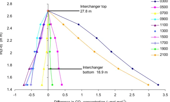
from the six measurement cycles) were plotted against ln(z – d), where z is height of measurement and d is the zero plane displacement, taken as a constant 13 m, based on previous measurements of wind speed profiles (Stewart and Thom, 1973) . Most of the time good straight lines resulted, leading to reliable estimates of the net CO2 flux. Examples

of hourly [CO2] profiles during a day are shown in Fig. 1.

Soil moisture measurements. The soil moisture content was measured once every few days using a neutron probe (Bell, 1969) at depths of 0.2, 0.35, 0.5, 0.8 and 1.1 m in 16 access tubes.

Leaf Area Index. The seasonal variation in leaf area index of the pine trees was measured by sampling the needle population on harvested and wind-thrown trees covering the range of girth sizes (Beadle et al., 1982). The LAI of the bracken was measured on sampled fronds with a planimeter (Roberts et al., 1980). 1.4 1.6 1.8 2 2.2 2.4 2.6 2.8 -1 -0.5 0 0.5 1 1.5 2 2.5 3 3.5

Difference in CO2 concentration (Pmol mol-1)

ln (z -d ) (l n m ) 0300 0500 0700 0900 1100 1300 1500 1700 1900 2100 Interchanger top 27.8 m Interchanger bottom 18.9 m

Fig. 1. An example of the mean hourly CO2 concentration profiles on 16th June; night-time emission to the right, daytime uptake to the left.

Some hours only are shown for clarity. The lines shown join the concentrations at the different heights; they are not fitted. Every hour of data was individually inspected; lines drawn through the points were used in some instances but in most cases the mean difference in concentration between 27.8 and 18.9 m was read directly from the computed hourly output. In general, resolution of the mean hourly difference in [CO2] represented by the slopes of the profiles was better than +/- 0.03 mmol mol-1_.

Leaf wetness. Leaf wetness was assessed using 48 artificial leaves consisting of strips of printed circuit board exposed in the forest canopy. The resistance between parallel strips of copper was measured; when the surface was wet the resistance decreased dramatically.

Other measurements. There was a large number of other instruments making ancillary supporting measurements on the site (for details see McNeil and Shuttleworth, 1975; Oliver, 1975; Gash and Stewart, 1975; Stewart, 1988).

The data resource

Between March and October, 914 hours of data were collected on a total of 65 days. 37 hours of data were rejected because of evident instrument failure, giving 877 hours of potentially useful data. Of those, a further 167 were rejected for the following reasons. Firstly, during and after appreciable rainfall there was so much water on the canopy and thermometer shields that the interchanger measurements of specific humidity were inaccurate, leading to spurious Bowen ratios. Secondly, some hours of data were also rejected at dawn and dusk, at which times the available energy, potential temperature gradient and Bowen ratio all change sign. If the change of signs is not synchronous and

is spread over more than one hour, the derived values of ga

will be negative. Furthermore, as the Bowen ratio passes through zero, the algebraic solution (Eqns. 3 and 4 above) becomes undefined. This left an elite set of 710 hours of data, from which the following, key, flux-related measurements were abstracted: average interchanger Bowen ratio, total interchanger potential temperature difference (18.9 to 27.8 m), and CO2 concentration difference D[CO2]

over the same height interval. The last was derived from the [CO2] profiles, as shown in Fig. 1. Hourly values of the

following descriptive variables were also abstracted for use in this analysis: hour number, date, surface wetness, air temperature, wind-speed, specific humidity deficit, D, solar radiation, Q, and available energy, A.

Results

The weather during the measurements. The period from March to October has been divided into spring, summer and autumn periods, for which there are 23, 24 and 18 days of flux data, respectively. Figure 2 shows ensemble means of the four most relevant weather variables (Q, A, T and D) for the three seasons. Whilst ensemble means do hide the extremes, they show clearly the daily and monthly changes over the seasons. The consistently high values of solar

(g k D 4 -100 0 100 200 300 400 500 600 700 1 6 11 16 21 Hour of day Q (W m -2) Mar_May Jun_Aug Sep_Oct -100 0 100 200 300 400 500 600 700 1 6 11 16 21 Hour of day A (W m -2) Mar_May Jun_Aug Sep_Oct 0 2 6 8 10 12 1 6 11 16 21 Hour of day g -1) Mar_May Jun_Aug Sep_Oct 0 5 10 15 20 25 1 6 11 16 21 Hour of day T ( oC) Mar_May Jun_Aug Sep_Oct

Fig. 2. Daily ensemble means of solar radiation (Q), available energy (A), air temperature above the canopy (T) and specific humidity deficit (D) above the canopy for three periods of the year. The ensembles were obtained from the original, complete data-set by binning the hourly values for each of the variables for each hour of the days in the seasonal periods indicated. The number of values represented by each point varies between 6 and 24. There were fewest observations overnight and fewer at the start and end of each day than in the middle of the day.

radiation, available energy, temperature and humidity deficit in the summer period are very evident.

CO2 flux in relation to time of day. Specimen daily CO2

fluxes at different times of the year are shown in Fig. 3. As the seasons progress, the CO2 flux increases in duration and

size as the days lengthen and the solar radiation increases. There is a clear correlation between CO2 fluxes and Q for

these days of moderate D (< 10 g kg–1_{). However, on days}

when D becomes larger (> 10 g kg–1_{) during the morning,}

the CO2 flux starts a decline that continues throughout the

remainder of the day (Table 1). This decline in Fc at large D

(>10 g kg–1_{) is just visible on the last day shown for August}

in Fig 3 (lower panel) and is evident in the relatively small fluxes at high Q visible in the data from June–August shown in Fig. 5.

Seasonal change in CO2 flux. Using ensemble means, Fig.

4 shows the seasonal variation in Fc and E. Somewhat

surprisingly, the CO2 fluxes reach ‘peaks’ of very similar

size in the three seasons but the effect of day length clearly limits the area between the curves and the base line. By contrast, E shows a strong seasonal variation, most likely because of its much stronger positive dependence on D than

on available energy (or solar radiation) because of the strong aerodynamic coupling to the atmosphere of pine forest (Jarvis and McNaughton, 1986).

Discussion

CO2 FLUX IN RELATION TO WEATHER VARIABLES

Figure 5 shows the scatter of the entire population of data points of the CO2 and water vapour fluxes in relation to

solar radiation, available energy and specific humidity deficit, identified by colour with respect to the three seasons. Clearly it is difficult to derive a great deal of sense from the data by inspection. Employing a model is desirable to extract the most information. However, the use of ensemble means gives a fair indication of the practically important variables. Ensemble means of the data in Fig. 5, sorted by season, are shown in Fig. 6. It is clear from Fig. 6 that Fc closely follows

solar radiation up to Q of c. 550 W m–2_{. There are practically}

no values of Q higher than 550 W m–2 _{in spring and autumn,}

but in summer Q reached 857 W m–2 _{on 8th June and 10th}

July. At Q>550 W m–2_{, there are not as many values of F} c

per point as at Q<550 W m–2_{, and that may account for some}

of the waywardness in the relationship. In addition, it is

Fig. 3. Seasonal diurnal plots of specimen days on 31st _{March, 11}th _{June and 21}st _{September (upper panel) and a sequence of days in August}

(4th_-6th _{and 9}th_-11th_{) (lower panel). The August data show days for which data were collected nearly continuously over 24 hours, but note that}

there is a gap between 1900 hrs on the 6th _{and 0400 hrs on the 9}th_.

-30 -25 -20 -15 -10 -5 0 5 10 15 4 8 12 16 20 Fc (P mo l m -2 s -1 ) o r D (g k g -1 ) March 4 8 12 16 20 Hour of day June -30 -25 -20 -15 -10 -5 0 5 10 15 4 11 17 23 5 11 17 23 6 12 18 9 15 22 4 10 16 22 4 10 16 Hour of day Fc (P mo l m -2 s -1 ) o r D (g kg -1 ) -100 0 100 200 300 400 500 600 700 800 Q ( W m -2 ) D Fc Q August 4 8 12 16 20 -100 0 100 200 300 400 500 600 700 800 Q (W m -2 ) Sept

-0.02 -0.01 0 0.01 0.02 0.03 0.04 0.05 0.06 1 6 11 16 21 Hour of day E (g m -2 s -1) Mar_May Jun_Aug Sep_Oct -20 -15 -10 -5 0 5 10 1 6 11 16 21 Hour of day Fc (P mo l m -2 s -1) Mar_May Jun_Aug Sep_Oct

Fig. 4. Daily ensemble means of the elite data set of CO2 flux (Fc) and evaporation rate (E) for spring, summer and autumn. The ensemble

means were obtained by binning the hourly values for each of the variables for each hour of the days in the monthly periods indicated. The number of values represented by each point varies between 6 and 24. There were fewest observations overnight and fewer at the start and end of each day than in the middle of the day.

-40 -30 -20 -10 0 10 20 -100 100 300 500 700 900 Q (W m-2 ) Fc (P mo l m -2 s -1) Mar_May Jun_Aug Sep_Oct -0.02 0.00 0.02 0.04 0.06 0.08 0.10 -100 100 300 500 700 900 A (W m-2 ) E (g m -2 s -1) Mar_May Jun_Aug Sep_Oct -0.02 0.00 0.02 0.04 0.06 0.08 0.10 0 5 10 15 20 25 D (g kg-1₎ E (g m -2 s -1) Mar_May Jun_Aug Sep_Oct -40 -30 -20 -10 0 10 20 -0.02 0.00 0.02 0.04 0.06 0.08 0.10 E (g m-2 s-1) Fc ( P mo l m -2 s -1) Mar_May Jun_Aug Sep_Oct

Fig. 5. Scatter plots of the CO2 flux (Fc) in relation to the solar radiation radiation (Q) and the evaporation rate (E) (right side); and between

the evaporation rate (E) and the available energy (A) and the specific humidity deficit (D) (left side). The source dataset is identical to that used in Fig. 4, and is similarly separated into spring, summer and autumn.

likely that Fc may become saturated with respect to Q at

such high irradiances. However, high values of Q are correlated with high temperatures and thus with large D which, as seen earlier (Table 1), leads to severe reduction in Fc, and this is also likely to be part of the reason for the

somewhat erratic levelling off of Fc.

The ensemble mean of the evaporation flux also shows a

good correlation with available energy, A, up to about 300 W m–2_{,beyond which the spring and autumn data diverge}

from the summer data. Evaporation in all three seasons is well correlated with D up to c. 10 g kg–1_{, beyond which the}

summer data continue erratically, without further systematic increase in E.

response of canopy (stomatal) conductance (gc), as

elucidated by Stewart (1988), based on analysis of the interchanger data for dry days, and by Beadle et al. (1985c) based on extensive porometer measurements within the canopy. They found that the canopy conductance declines drastically as D increases, reaching low values at D > c. 10 g kg–1 _{and thereby accounting for the lack of further increase}

in both E and Fc. Based on his earlier analysis of evaporation

data on completely dry days (Stewart, 1988), the concurrent reductions in CO2 flux and evaporation can largely be

attributed to decrease in canopy conductance. One consequence of this is that Fc has a close relationship with

E as shown in Fig. 6, and as was first shown long ago by Monteith (1963) for field crops.

Treating the relationship as linear, the ratio of E/Fc (= j)

in comparable units is approximately 195 mol of H2O

evaporated per mol of CO2 assimilated, or 80 g of H2O per

g of CO2. Analogous values of j in the range 100 to 200

were found for Sitka spruce at Fetteresso Forest, but larger values of 400 to 500 for oak–hickory woodland in Tennessee, in all three cases in average weather conditions; much larger values of j were found at low Q or large D; and values for crops were also in general larger (Jarvis, 1986). Clearly, assessing j on the basis of ensemble means

hides a great deal of significant variation in the relationship. Jarvis (1986) modelled j in relation to Q, D, T and gc to

understand what was controlling its variation. E is strongly dependent on gc and D (both positively and negatively) and

to a lesser extent on A; Fc depends strongly on Q and to a

lesser extent on gc and T (both positively and negatively

through its impacts on both carbon assimilation and tree and soil respiration). This data set provides an opportunity for further exploration of the coefficient j in relation to the quite extreme conditions that occurred, making use of the better models now available.

The contribution that the bracken might be making to the water and CO2 fluxes should also be considered. Its LAI

adds considerably to that of the pine canopy, increasing the total LAI after bud burst to c. 3.6. Porometer measurements on the bracken (Roberts et al., 1980) showed a small bracken canopy conductance almost insensitive to D, contributing about 50% of the total canopy conductance gc when D > 8 g

kg–1_{. Calculations by Roberts et al. (1980) indicate that the}

bracken contributed around 20% of E in June and September, but that the relative contribution increased as D increased, reaching a maximum of 65% of E in the extreme conditions on the 9th of July. This increase in the role of the bracken occurs because increase in D causes relatively more

Fig. 6 Ensemble means of the CO2 flux (Fc) in relation to the solar radiation (Q) and the evaporation rate (E) (right side); and between the

evaporation rate (E) and the available energy (A) and the specific humidity deficit (D) (left side) for the same data set as in Figure 5. The number of values represented by each point varies between 6 and 24. The ensembles were obtained by sorting the hourly values of the fluxes into bins of the variables. There were fewest observations overnight and fewer at the start and end of each day than in the middle of the day.

-0.01 0 0.01 0.02 0.03 0.04 0.05 0.06 -100 100 300 500 700 900 A (W m-2₎ E (g m -2 s -1) Mar_May Jun_Aug Sep_Oct -20 -15 -10 -5 0 5 10 -100 100 300 500 700 900 Q (W m-2₎ Fc ( P mo l m -2 s -1) Mar_May Jun_Aug Sep_Oct -20 -15 -10 -5 0 5 10 0 0.02 0.04 0.06 0.08 E (g m-2 s-1₎ Fc ( P mo l m -2 s -1) Mar_May Jun_Aug Sep_Oct -0.01 0 0.01 0.02 0.03 0.04 0.05 0.06 0 5 10 15 20 D (g kg-1₎ E g m -2 s -1) Mar_May Jun_Aug Sep_Oct

reduction in the pine shoot conductance (Beadle et al., 1985) and in the overall forest conductance, gc (Stewart 1988) than

in the bracken conductance, which is relatively insensitive to D.

The Thetford Scots pine results can be compared with similar data for the younger, denser stand of Sitka spruce (Picea sitchensis (Bong.) Carr.) (with no understorey) obtained in 1973 during the Fetteresso Project, in the somewhat more oceanic climate of eastern Scotland, where a very similar approach and some of the same technology was used (Jarvis, 1994). The Sitka spruce stand showed appreciably larger daytime CO2 fluxes reaching 30 mmol

m–2 _s–1_{, in conditions of Q c. 700 W m}-2_{, T c. 15} o_{C and D <}

10 g kg–1_{. But with T> 20}o_{C and D > 15 g kg}–1_{, there were}

analagous, but stronger, reductions in gc, accompanied by

large reductions in Fc, which went positive or hovered

around zero for much of the day; i.e. the results were very similar to those for Scots pine at Thetford but the physiological responses were triggered by less extreme conditions (Jarvis, 1994). More comprehensive data on Sitka spruce, obtained more recently in central Scotland within the EU EUROFLUX programme using eddy covariance, endorse these results and provide greater opportunities for analysis (Clement, 2004).

The results from Thetford can also be compared with the exchanges of other stands of predominantly Scots pine that have been investigated in more continental climates within the EU EUROFLUX programme, using the eddy-covariance methodology (Ceulemans et al., 2003). Ensemble means for CO2 fluxes in July 1997 peaked at –9, –10, –11

and –19 mmol m–2 _s–1 _{for sites in Belgium, The Netherlands,}

Finland and Sweden, respectively. That is, the fluxes in these stands are of similar magnitude but smaller than those at Thetford, where Fc reached 20 mmol m–2 s–1, in moderate

conditions. One advantage of the eddy-covariance methodology is that the measurement is independent of the energy and humidity fluxes so that CO2 fluxes can be

measured at night, albeit with some other potential problems. For the continental sites, the ensemble mean night time fluxes for July data 1997 lie between 2 and 8 mmol m–2 _s–1_.

For those few days for which there are 24-hourThetford data, for example the August data shown in Fig. 3, the night-time fluxes lie between 5 and 10 mmol m–2 _s–1_{. Thus in}

general the Scots pine stand in Thetford forest in 1976 was functioning in a similar manner to contemporary, more continental, European Scots pine stands, but with larger fluxes and greater sensitivity to periods of extreme atmospheric specific humidity deficit. This may be a portent for forests of Scottish provenance in England with respect to the projected increases in atmospheric temperature.

Conclusions

(1) High air temperatures of 25 to 30o_{C led to large specific}

humidity deficits, which caused severe reductions in CO2 uptake, as well as in evaporation.

(2) There was rapid recovery in both CO2 uptake and

evaporation when specific humidity deficits dropped below c. 15 g kg–1_{, generally as a result of lower air}

temperatures, rather than lower irradiance, indicating that the large soil water deficit was not the main cause of the reductions.

(3) In conditions of moderate temperature and specific humidity deficit and high solar irradiance, the rate of CO2 uptake reached 20 mmol m–2 s–1, a higher rate than

recently found for four pine forests in continental Europe during July 1997.

(4) The air temperature, specific humidity deficit and soil water deficit in 1976 were quite exceptional and similar conditions were probably not experienced again until 2003. Thus the information gained at Thetford in 1976 on the response of the forest ecosystem may provide a good guide to the response of English pine forests to climate change over the next 25 years.

(5) There is still more valuable information to be obtained from the 1976 Thetford data with respect to the likely impacts of the projected climate change.

Acknowledgements

Oliver Beveridge is thanked for carefully entering the data into Excel and Sylvia Oliver for help with interpretation of the original Teleprinter output.

References

Beadle, C.L., Talbot, H. and Jarvis, P.G., 1982. Canopy structure and leaf area index in a mature Scots pine forest. Forestry, 55, 105–123.

Beadle, C.L., Neilson, R.E., Talbot, H. and Jarvis, P.G., 1985a. Stomatal conductance and photosynthesis in a mature Scots pine forest. I. Diurnal, seasonal and spatial variation in shoots. J. Appl. Ecol., 22, 557–571.

Beadle, C.L., Jarvis, P.G., Talbot, H. and Neilson, R.E., 1985b. Stomatal conductance and photosynthesis in a mature Scots pine forest. II. Dependence on environmental variables of single shoots. J. Appl. Ecol., 22, 573–586.

Beadle, C.L., Talbot, H., Neilson, R.E. and Jarvis, P.G., 1985c. Stomatal conductance and photosynthesis in a mature Scots pine forest. III. Variation in canopy conductance and canopy photosynthesis. J. Appl. Ecol., 22, 587–595.

Bell, J.P., 1969. A new design principle for neutron soil moisture gauges: the Wallingford Neutron Probe. Soil Science, 103, 160– 164.

Ceulemans, R., Kowalski, A.S., Berbigier, P., Dolman, H., Grelle, A., Janssens, I.A., Lindroth, A., Moors, E., Rannik, U. and Vesala, T., 2003. 5. Coniferous forests (Scots and maritime pine):

carbon and water fluxes, balances, ecological and ecophysiological determinants. In: Fluxes of Carbon, Water and Energy of European Forests, R. Valentini (Ed.), Springer-Verlag, Berlin, Germany. 71–97.

Ciais, Ph. and 32 others, 2005. Europe-wide reduction in primary productivity caused by the heat and drought in 2003. Nature,

437, 529–533.

Clement, R.J., 2004. Mass and energy exchange of a plantation forest in Scotland using micrometeorological methods. Ph.D. Thesis, The University of Edinburgh, 496 pp.

Cooper, J.D., 1980. Measurement of fluxes in unsaturated soil in Thetford Forest. Institute of Hydrology Report No. 66, 97 pp. Corbett, W.M., 1973. Breckland Forest Soils. The Soil Survey.

Rothamsted Experimental Station, 120 pp.

Denmead, O.T. and McIlroy, I.C., 1971. Measurement of carbon dioxide exchange in the field. In: A Manual of Photosynthetic Methods, Z. Sestak, J. Catský,. and P.G. Jarvis, (Eds.), Dr. W. Junk NV, The Hague. 467–516.

Gash, J.H.C. and Stewart J.B., 1975.The average surface resistance of a pine forest derived from Bowen ratio measurements. Bound.-Layer Meteorol., 8, 453–464.

Jarvis, P.G., 1976. The interpretation of the variations in leaf water potential and stomatal conductance found in canopies in the field. Phil. Trans. R. Soc. London, Ser. B, 273, 593–610. Jarvis, P.G., 1981. Production efficiency of coniferous forest in

the UK. In: Physiological Processes Limiting Plant Productivity, C.B. Johnson, (Ed.), Butterworth Scientific Publications, London. 81–107.

Jarvis, P.G. (with an Appendix by P.G. Jarvis & Y.-P. Wang), 1986. Coupling of carbon and water interactions in forest stands. Tree Physiol., 2, 347–368.

Jarvis, P.G., 1994. Capture of carbon dioxide by coniferous forest. In: Resource Capture by Crops, J.L. Monteith, R.K. Scott and M.H. Unsworth, (Eds.), Nottingham University Press, Nottingham, UK. 351–374.

Jarvis, P.G. and Sandford, A.P., 1985. The measurement of carbon dioxide in air. In: Instrumentation for Environmental Physiology, B. Marshall and F.I. Woodward, (Eds), CUP, Cambridge, UK. 29–57.

Jarvis, P.G. and McNaughton, K.G., 1986. Stomatal control of transpiration: scaling up from leaf to region. Adv. Ecology Res.,

15, 1–49.

Jarvis, P.G., James, G.B. and Landsberg, J.J., 1976. Coniferous Forest. In: Vegetation and The Atmosphere, Volume 2, Case Studies, J.L. Monteith, (Ed.), Academic Press, New York, USA. 171–240.

McNeil, D.D. and Shuttleworth, W.J., 1975. Comparative measurements of the energy fluxes over a pine forest. Bound.-Layer Meteorol., 9, 297–313.

Monteith, J.L., 1963. Gas exchange in plant communities. In: Environmental Control of Plant Growth, L.T. Evans (Ed.), Academic Press, New York, USA. 95–112.

Oliver, H., 1975. Ventilation in a forest. Agr. Meteorol., 14, 347– 355.

Parkinson, K.J. and Legg, B.J., 1978. Calibrations of infra-red analysers for carbon dioxide. Photosynthetica, 12, 65–67. Roberts, J.M., 1976. A study of root distribution and growth in a

Pinus sylvestris L. plantation in East Anglia. Plant and Soil,

44, 607–621.

Roberts, J., Pymar, C.F., Wallace, J.S. and Pitman, R.M., 1980. Seasonal changes in leaf area, stomatal and canopy conductances and transpiration from bracken below a forest canopy. J. Appl. Ecol., 17, 409–422.

Stewart, J.B., 1978. A micrometeorological investigation into the factors controlling the evaporation from a forest. Ph.D. Thesis, Reading University, 211 pp.

Stewart, J.B., 1988. Modelling the surface conductance of pine forest. Agr. Forest Meteorol., 43, 19–35.

Stewart, J.B. and Thom, A.S., 1973. Energy budgets in pine forest. Quart. J. Roy. Meteorol. Soc., 99, 164–170.