HAL Id: hal-00296446
https://hal.archives-ouvertes.fr/hal-00296446
Submitted on 14 Feb 2008
HAL is a multi-disciplinary open access
archive for the deposit and dissemination of
sci-entific research documents, whether they are
pub-lished or not. The documents may come from
teaching and research institutions in France or
abroad, or from public or private research centers.
L’archive ouverte pluridisciplinaire HAL, est
destinée au dépôt et à la diffusion de documents
scientifiques de niveau recherche, publiés ou non,
émanant des établissements d’enseignement et de
recherche français ou étrangers, des laboratoires
publics ou privés.
of very large solar proton events
C. H. Jackman, D. R. Marsh, F. M. Vitt, R. R. Garcia, E. L. Fleming, G. J.
Labow, C. E. Randall, M. López-Puertas, B. Funke, T. von Clarmann, et al.
To cite this version:
C. H. Jackman, D. R. Marsh, F. M. Vitt, R. R. Garcia, E. L. Fleming, et al.. Short- and medium-term
atmospheric constituent effects of very large solar proton events. Atmospheric Chemistry and Physics,
European Geosciences Union, 2008, 8 (3), pp.765-785. �hal-00296446�
www.atmos-chem-phys.net/8/765/2008/ © Author(s) 2008. This work is licensed under a Creative Commons License.
Chemistry
and Physics
Short- and medium-term atmospheric constituent effects of very
large solar proton events
C. H. Jackman1, D. R. Marsh2, F. M. Vitt2, R. R. Garcia2, E. L. Fleming1, G. J. Labow1, C. E. Randall3, M. L´opez-Puertas4, B. Funke4, T. von Clarmann5, and G. P. Stiller5
1NASA/Goddard Space Flight Center, Greenbelt, MD, USA 2National Center for Atmospheric Research, Boulder, CO, USA 3University of Colorado, Boulder, CO, USA
4Instituto de Astrofisica de Andalucia, CSIC, Granada, Spain
5Institut f¨ur Meteorologie und Klimaforschung, Forschungszentrum Karlsruhe and Univ. Karlsruhe, Karlsruhe, Germany
Received: 26 June 2007 – Published in Atmos. Chem. Phys. Discuss.: 23 July 2007 Revised: 28 November 2007 – Accepted: 15 January 2008 – Published: 14 February 2008
Abstract. Solar eruptions sometimes produce protons, which impact the Earth’s atmosphere. These solar proton events (SPEs) generally last a few days and produce high energy particles that precipitate into the Earth’s atmosphere. The protons cause ionization and dissociation processes that ultimately lead to an enhancement of hydrogen and odd-nitrogen in the polar cap regions (>60◦ geomagnetic lati-tude). We have used the Whole Atmosphere Community Climate Model (WACCM3) to study the atmospheric im-pact of SPEs over the period 1963–2005. The very largest SPEs were found to be the most important and caused at-mospheric effects that lasted several months after the events. We present the short- and medium-term (days to a few months) atmospheric influence of the four largest SPEs in the past 45 years (August 1972; October 1989; July 2000; and October–November 2003) as computed by WACCM3 and observed by satellite instruments. Polar mesospheric NOx(NO+NO2) increased by over 50 ppbv and mesospheric
ozone decreased by over 30% during these very large SPEs. Changes in HNO3, N2O5, ClONO2, HOCl, and ClO were
in-directly caused by the very large SPEs in October–November 2003, were simulated by WACCM3, and previously mea-sured by Envisat Michelson Interferometer for Passive At-mospheric Sounding (MIPAS). WACCM3 output was also represented by sampling with the MIPAS averaging kernel for a more valid comparison. Although qualitatively similar, there are discrepancies between the model and measurement with WACCM3 predicted HNO3and ClONO2enhancements
being smaller than measured and N2O5enhancements being
larger than measured. The HOCl enhancements were fairly Correspondence to: C. H. Jackman
similar in amounts and temporal variation in WACCM3 and MIPAS. WACCM3 simulated ClO decreases below 50 km, whereas MIPAS mainly observed increases, a very perplex-ing difference. Upper stratospheric and lower mesospheric NOx increased by over 10 ppbv and was transported during
polar night down to the middle stratosphere in several weeks past the SPE. The WACCM3 simulations confirmed the SH HALOE observations of enhanced NOxin September 2000
as a result of the July 2000 SPE and the NH SAGE II ob-servations of enhanced NO2in March 1990 as a result of the
October 1989 SPEs.
1 Introduction
The Earth’s atmosphere is occasionally bombarded by a large flux of protons during solar proton events (SPEs). Although relatively infrequent, some of the especially large SPEs have been documented to have a substantial influence on chemical constituents in the polar middle atmosphere, especially HOx,
NOy, and ozone (e.g. Weeks et al., 1972; Heath et al., 1977;
Reagan et al., 1981; McPeters et al., 1981; Thomas et al., 1983; McPeters and Jackman, 1985; McPeters, 1986; Jack-man and McPeters, 1987; Zadorozhny et al., 1992; JackJack-man et al., 1995, 2001, 2005a; Randall et al., 2001; Seppala et al., 2004, 2006; L´opez-Puertas et al., 2005a, b; von Clarmann et al., 2005; Orsolini et al., 2005; Degenstein et al., 2005; Ro-hen et al., 2005; Verronen et al., 2006). The influx of solar protons during large events, which are more frequent near so-lar maximum, can strongly perturb the chemical composition of the polar middle atmosphere via ionization, dissociation, dissociative ionization, and excitation processes.
The important constituent families of HOx (H, OH,
HO2) and NOy (N(4S), N(2D), NO, NO2, NO3, N2O5,
HNO3, HO2NO2, ClONO2, BrONO2)are produced either
directly or through a photochemical sequence as a result of SPEs. The SPE-produced HOxconstituents are important in
controlling ozone in the upper stratosphere and mesosphere (pressures less than about 2 hPa). Short-term ozone destruc-tion via the HOxspecies proceeds through several catalytic
loss cycles such as OH+O3→HO2+O2
followed by HO2+O → OH + O2
Net: O+O3→O2+O2
and H+O3→OH+O2
followed by OH+O → H+O2
Net: O+O3→O2+O2.
The SPE-produced NOx (NO+NO2) constituents lead
to short- and longer-term catalytic ozone destruction in the lower mesosphere and stratosphere (pressures greater than about 0.5 hPa) via the well-known NOx-ozone loss cycle
NO+O3→NO2+O2
followed by NO2+O → NO+O2
Net: O+O3→O2+O2.
There have been a number of modeling studies focused on understanding and predicting the atmospheric influence of SPEs (e.g. Warneck, 1972; Swider and Keneshea, 1973; Crutzen et al., 1975; Swider et al., 1978; Banks, 1979; Fabian et al., 1979; Jackman et al., 1980, 1990, 1993, 1995, 2000, 2007; Solomon and Crutzen, 1981; Rusch et al., 1981; Solomon et al., 1981, 1983; Reagan et al., 1981; Jackman and McPeters, 1985; Roble et al., 1987; Reid et al., 1991; Vitt and Jackman, 1996; Vitt et al., 2000; Krivolutsky et al., 2001, 2003, 2005, 2006; Verronen et al., 2002, 2005, 2006; Seme-niuk et al., 2005). Most of these studies were carried out with lower dimensional models (0-D, 1-D, 2-D); however, a few used three-dimensional (3-D) models (e.g. Jackman et al., 1993, 1995, 2007; Semeniuk et al., 2005; Krivolutsky et al., 2006) to investigate the more detailed global effects of SPEs.
In this study we have used version 3 of the Whole Atmo-sphere Community Climate Model (WACCM3), which is a fully coupled general circulation with photochemistry model with a domain that extends from the ground to the lower thermosphere. WACCM3 allows study of the detailed time-dependent 3-D atmospheric response to a variety of pertur-bations. Earlier studies of SPEs with 3-D models focused
on single very large SPE periods. For example, Jackman et al. (1993, 1995) studied the October 1989 SPEs; Semeniuk et al. (2005) and Jackman et al. (2007) investigated the Oc-tober/November 2003 SPEs; and Krivolutsky et al. (2006) considered the July 2000 SPE. The purpose of this work is to use WACCM3 to investigate the global effects of four very large SPE periods over solar cycles 20–23 (years 1963– 2005), namely, the August 1972, October 1989, July 2000, and October 2003 SPEs. The atmosphere was undergoing substantial changes from 1963–2005 with ground chlorine source gas amounts increasing from about 0.9 to 3.3 ppbv and ground carbon dioxide amounts increasing from about 317 to 380 ppmv. Also, the SPE periods themselves were somewhat different with significant variations in the tem-poral and altitudinal extent and intensity of the particular events.
Some recent work (e.g., Jackman et al., 2001, 2005a; Ro-hen et al., 2005; Krivolutsky et al., 2006) has indicated that the observed NOxenhancements and ozone decreases during
and shortly after SPEs can be fairly reasonably simulated. However, recent measurements of SPE-caused short-term enhancements of HOCl, ClO, and ClONO2(von Clarmann
et al., 2005) and HNO3 and N2O5 (L´opez-Puertas et al.,
2005b) have not yet been compared with global model sim-ulations in the literature to the best of our knowledge. Also, the medium-term polar enhancements in NOxin September
2000 attributed to the July 2000 SPE (Randall et al., 2001) have not yet been modeled with a general circulation model as far as we know.
This investigation will focus on the short-and medium-term (days to months) atmospheric influence caused by the very large SPE periods in August 1972, October 1989, July 2000, and October–November 2003. We will compare our WACCM3 predictions with observations from several satel-lite instruments documenting SPE effects during these four periods. As part of this analysis we will discuss SPE-caused short-term enhancements in HNO3, N2O5, HOCl,
ClONO2, and ClO and compare WACCM3 and satellite
mea-surements in October–November 2003. We will also com-pare WACCM3 with observations of the medium-term NOx
enhancements caused by the SPEs (up to several months past the events). This study will ultimately provide a test of the ability of a general circulation model with chemistry to sim-ulate several different SPE periods.
This paper is divided into seven primary sections, includ-ing the Introduction. The solar proton flux and ionization rate computation are discussed in Sect. 2 and SPE-induced pro-duction of HOxand NOyare discussed in Sect. 3. A
descrip-tion of the satellite instrument measurements and WACCM3 is given in Sect. 4. WACCM3 model results for short-term (days) constituent changes, with comparisons to measure-ments for some very large SPEs of the past 45 years, are shown in Sect. 5 while medium-term (months) constituent changes caused by SPEs are discussed in Sect. 6. The con-clusions are presented in Sect. 7.
2 Proton measurement/ionization rates
Solar proton fluxes have been measured by a number of satel-lites in interplanetary space or in orbit around the Earth. The National Aeronautics and Space Administration (NASA) In-terplanetary Monitoring Platform (IMP) series of satellites provided measurements of proton fluxes from 1963–1993 (Jackman et al., 1990; Vitt and Jackman, 1996). The Na-tional Oceanic and Atmospheric Administration (NOAA) Geostationary Operational Environmental Satellites (GOES) were used for proton fluxes from 1994–2005 (Jackman et al., 2005b).
Proton flux data from IMP 1–7 were used for the years 1963–1973. These data were taken from T. Armstrong and colleagues (University of Kansas, private communication, 1986; see Armstrong et al. (1983) for a discussion of the IMP 1–7 satellite measurements). A power law was used to fit these flux data as a function of energy, which were as-sumed to be valid over the range 5–100 MeV (Jackman et al., 1990) and then degraded in energy using the scheme first discussed in Jackman et al. (1980). The scheme includes the deposition of energy by all the protons and associated sec-ondary electrons. The energy required to create one ion pair was assumed to be 35 eV (Porter et al., 1976).
IMP 8 was used for the proton flux data for the years 1974– 1993. Vitt and Jackman (1996) take advantage of the mea-surements of alpha particles by IMP 8 as well and use pro-ton fluxes from 0.38–289 MeV and alpha fluxes from 0.82– 37.4 MeV in energy deposition computations. The energy deposition methodology is similar to that discussed in Jack-man et al. (1980). Alpha particles were found to add about 10% to the total ion pair production during SPEs.
Four GOES satellites are used for the proton fluxes in years 1994–2005: 1) GOES-7 for the period 1 January 1994 through 28 February 1995; 2) GOES-8 for the period 1 March 1995 through 8 April 2003, and 10 May 2003 to 18 June 2003; 3) GOES-11 for the period 19 June 2003 to 31 December 2005; and 4) GOES-10 to fill in the gap of miss-ing proton flux data from 9 April through 9 May 2003. The GOES satellite proton fluxes are fit with exponential spec-tral forms in three energy intervals: 1–10 MeV, 10–50 MeV, and 50–300 MeV. The energy deposition methodology again is that discussed in Jackman et al. (1980).
There are uncertainties associated with these proton fluxes, especially given the large number of satellite instruments used to compile the measurement record. We have made some straightforward comparisons of particular proton flux measuring instruments and estimate the proton flux uncer-tainties to be up to 50%. Although it is beyond the scope of the present study to undertake a more detailed comparison, we recommend that such an investigation be accomplished by experts in the field of solar particle observations.
The daily average ion pair production rates for years 1963– 2005 were computed from the energy deposition assuming 35 eV/ion-pair. An example of the daily average ionization
Fig. 1. Daily average ion pair production rates using the GOES 11 proton flux measurements for 26 October through 7 Novem-ber 2003. Contour levels are 100, 200, 500, 1000, 2000, and 5000 cm−3s−1.
rate (cm−3s−1)is given in Fig. 1 for a thirteen day period
in October–November 2003, a very intense period of SPEs. The 28–31 October 2003 SPE period was the fourth largest of the past 45 years (see Table 1). Very large daily aver-age ionization rates of >5000 cm−3s−1extending from 0.01
to 1 hPa are computed for 29 October 2003. Large ioniza-tion rates >1000 cm−3s−1extending from the upper
strato-sphere through the mesostrato-sphere are computed for 28–30 Oc-tober 2003.
These ionization rate data are provided as functions of pressure between 888 hPa (∼1 km) and 8×10⁻⁵hPa
(∼115 km) at the SOLARIS (Solar Influence for SPARC) website (http://www.geo.fu-berlin.de/en/met/ag/strat/ research/SOLARIS/Input data/index.html) and can be used in model simulations.
3 Odd hydrogen (HOx) and odd nitrogen (NOy)
pro-duction
3.1 Odd hydrogen (HOx)production
Protons and their associated secondary electrons produce odd hydrogen (HOx). The production of HOx takes place after
the initial formation of ion-pairs and is the end result of com-plex ion chemistry (Swider and Keneshea, 1973; Frederick, 1976; Solomon et al., 1981). Generally, each ion pair results in the production of approximately two HOxspecies in the
upper stratosphere and lower mesosphere. In the middle and upper mesosphere, an ion pair is calculated to produce less than two HOx species. The HOx production from SPEs is
included in WACCM3 using a lookup table from Jackman et al. (2005a, Table 1), which is based on the work of Solomon et al. (1981). The HOx constituents are quite reactive with
each other and with other constituents and have a relatively short lifetime (∼hours) throughout most of the mesosphere
Table 1. Largest 15 Solar Proton Event Periods in Past 45 Years.
Date of SPE(s) Rank Computed NOyProduction
In Middle Atmosphere (Gigamoles1) 19–27 October 1989 1 11. 2–10 August 1972 2 6.0 14–16 July 2000 3 5.8 28–31 October 2003 4 5.6 5–7 November 2001 5 5.3 9–11 November 2000 6 3.8 24–30 September 2001 7 3.3 13–26 August 1989 8 3.0 23–25 November 2001 9 2.8 2–7 September 1966 10 2.0 15–23 January 2005 11 1.8 29 September–3 October 1989 12 1.7 28 January–1 February 1967 13 1.6 23-29 March 1991 14 1.5 7–17 September 2005 15 1.5
1Gigamole=6.02×1032atoms and molecules
NOy Production; Sunspot No.
1965 1975 1985 1995 2005 Year NO y production (Gigamoles/year) SPE source 10-4 10-3 10-2 10-1 100 101 102 0 50 100 150 200 0 Sunspot Number SC SC SC SC 20 21 22 23
Fig. 2. The NOyproduction (gigamoles per year) in the middle
at-mosphere by SPEs is indicated by the histogram with the left ordi-nate showing the scale; the annual averaged sunspot numbers are in-dicated by the dashed line with the right ordinate showing the scale; and the number of the solar cycle (SC) is also indicated (SC 19, SC 20, SC 21, SC 22, SC 23). Plotted values for NOyproduction
are taken from Jackman et al. (1980, 1990, 2005b), Vitt and Jack-man (1996), and recent computations.
(Brasseur and Solomon, 1984, see Fig. 5.28) and thus are important only during and shortly after solar events. 3.2 Odd nitrogen (NOy)production
Odd nitrogen is produced when the energetic charged par-ticles (protons and associated secondary electrons) collide with and dissociate N2. We assume that ∼1.25 N atoms are
produced per ion pair and divide the proton impact of N atom production between ground state (∼45% or ∼0.55 per ion pair) and excited state (∼55% or ∼0.7 per ion pair) nitrogen atoms (Porter et al., 1976). Following the discussion in Jack-man et al. (2005a), we assume production of 0.55 ground state N(4S) atoms per ion pair and 0.7 N(2D) atoms per ion pair for our model simulations.
SPEs can also lead to a reduction in odd nitrogen via production of N(4S), when the NOy loss reaction,
N(4S)+NO→N2+O, is increased. This NOy loss
mecha-nism is important during especially large SPEs, when a huge amount of NOyis produced in a short period of time (Rusch
et al., 1981). In spite of the associated enhanced loss of NOy
during these disturbed periods, SPEs usually lead to a net increase in NOy. Figure 2 shows a time series of our
com-puted annually averaged global NOyproduction from SPEs
in the middle atmosphere. The NOyproduction roughly
fol-lows the solar cycle with maximum (minimum) production near sunspot maximum (minimum).
Although the solar UV-induced oxidation of nitrous oxide (N2O+O(1D)→NO+NO) provides the largest source of NOy
in the middle atmosphere (52–58 gigamoles per year; Vitt and Jackman 1996), the SPE source of NOy can be
signifi-cant during certain years. This is especially true at polar lati-tudes where the transport from lower latilati-tudes and the larger solar zenith angles result in a somewhat smaller local source of NOydue to N2O oxidation. Table 1 shows the magnitude
of the fifteen largest individual SPEs, in terms of the com-puted middle atmospheric NOy production, during the past
45 years. Note that eight of these event periods occurred during the current solar cycle (1996–2007).
The NOy family has a lifetime of months to years in the
middle and lower stratosphere (e.g. Randall et al., 2001; Jackman et al., 2005a). Therefore, the effects of the SPE-produced NOycan last for several months, especially when
large solar events occur in late fall or winter.
4 Model and measurement information
4.1 Description of the Whole Atmosphere Community Cli-mate Model (WACCM3)
The Whole Atmosphere Community Climate Model is based on the National Center for Atmospheric Research’s Commu-nity Atmospheric Model (CAM). The current version of the model, WACCM3, is derived from CAM, version 3 (CAM3), and includes all the physical parameterizations of that model. A description of CAM3 is given in Collins et al. (2004), which details the governing equations, physical parameter-izations and numerical algorithms. The reader is referred to the CAM Web site (http://www.ccsm.ucar.edu/models/ atm-cam/) for more information.
WACCM3 has fully interactive dynamics, radiation, and chemistry. WACCM3 not only incorporates modules from CAM3, but also the Thermosphere-Ionosphere-Mesosphere-Electrodynamics General Circulation Model (TIME-GCM) and the Model for OZone And Related chemical Tracers (MOZART-3). WACCM3 is a global model and has 66 verti-cal levels from the ground to 4.5×(10−6) hPa (approximately
145 km geometric altitude). Vertical resolution is ≤1.5 km between the surface and about 25 km. Above that altitude, vertical resolution increases slowly to 2 km at the stratopause and 3.5 km in the mesosphere; beyond the mesopause, the vertical resolution is one half the local scale height. The lat-itude and longlat-itude grids have spacing of 4◦and 5◦, respec-tively.
WACCM3 incorporates most of the CAM3 ingredients, however, its gravity wave drag and vertical diffusion param-eterizations are modified somewhat and described in Garcia et al. (2007). WACCM3 differs from CAM3 in other ways in that it includes a detailed neutral chemistry model for the middle atmosphere; heating due to chemical reactions; a model of ion chemistry in the mesosphere/lower thermo-sphere (MLT); ion drag and auroral processes; and parame-terizations of shortwave heating at extreme ultraviolet (EUV) wavelengths and infrared transfer under nonlocal thermody-namic equilibrium (NLTE) conditions. WACCM3’s neutral chemistry module including reactions and solver is described in Kinnison et al. (2007). The neutral constituent photo-chemical reaction rates and photodissociation cross sections are taken from Sander et al. (2003). As a full GCM with chemistry, WACCM3 implicitly includes the diurnal cycle for all constituents at all levels in the model’s domain. The other processes and parameterizations, which are unique to WACCM3, are described in Garcia et al. (2007). Other
de-tails about WACCM3 and model results are given in Sassi et al. (2002, 2004), Forkman et al. (2003), Richter and Garcia (2006), and Marsh et al. (2007).
4.2 WACCM3 simulations
WACCM3 was forced with observed time-dependent sea sur-face temperatures (SSTs), observed solar spectral irradiance and geomagnetic activity changes, and observed concentra-tions of greenhouse gases and halogen species over the simu-lation periods (see Garcia et al., 2007). We have completed a number of WACCM3 simulations, either with or without the daily ionization rates from SPEs. The ionization rates, when included, were applied uniformly over both polar cap regions (60–90◦N and 60–90◦S geomagnetic latitude) as solar pro-tons are guided by the Earth’s magnetic field lines to these areas (McPeters et al., 1981; Jackman et al., 2001, 2005a). The effects are not expected to be symmetric between the hemispheres because of the differing offsets of geomagnetic and geographic poles. Other differences between the hemi-spheres are primarily driven by seasonal differences in the northern and southern polar regions. Transport and solar an-gle disparities due to seasonal changes are the main causes of these inter-hemispheric variances.
A list of the WACCM3 simulations and their designation in this study is given in Table 2. Usually an ensemble consist-ing of four simulations with different initial conditions was run for each experiment. Simulation 1(a, b, c, d) with SPEs covered the full period 1 January 1963–31 December 2005. Since the year 1989 was very active in terms of SPEs (see Table 1), simulations with SPEs (see 2a, b, c, d) and with-out SPEs (see 2w, x, y, z) were performed to study the 16 month period, 1 January 1989–30 April 1990. The very large July 2000 SPE was studied in further detail over the period 2 July–30 September 2000 using simulations with SPEs (see 3a, b, c, d) and without SPEs (see 3w, x, y, z). The very large late October/early November 2003 SPEs were studied in fur-ther detail over the period 25 October–14 November 2003 using a simulation with SPEs (see 4a) and without SPEs (see 4w). Simulations 5(w, x, y, z) without SPEs run over the period 2 July 2000–31 December 2004 provided necessary daily information for computing the statistical significance of the WACCM3 results as a function of latitude and altitude. Throughout the paper we discuss 2σ statistical significance levels to illustrate how the SPE effects compares to the back-ground variability simulated in the model.
Simulations 1(a, b, c, d), 2(a, b, c, d), and 2(w, x, y, z) have model output every five days. Simulations 3(a, b, c, d), 3(w, x, y, z), 4(a), 4(w), and 5(w, x, y, z) have model output every day. For short periods (∼two weeks), different real-izations produce similar results; thus it is appropriate to use only a single realization for simulation 4. WACCM3 output, whether daily or every five days, is a snap-shot of model re-sults at 00:00 GMT.
Table 2. Description of WACCM3 simulations. Simulation designation Number of realizations Time period SPEs included 1 (a, b, c, d) 4 1963–2005 Yes
2 (a, b, c, d) 4 1 January 1989–30 April 1990 Yes 2 (w, x, y, z) 4 1 January 1989–30 April 1990 No 3 (a, b, c, d) 4 2 July–30 September 2000 Yes 3 (w, x, y, z) 4 2 July–30 September 2000 No 4 (a) 1 25 October–14 November 2003 Yes 4 (w) 1 25 October–14 November 2003
5 (w, x, y, z) 4 2 July 2000–31 December 2004 No
4.3 Satellite instrument measurements
Several satellite instruments have recorded atmospheric con-stituent change caused by SPEs. We will compare WACCM3 results with:
1. Nimbus 4 Backscatter Ultraviolet (BUV) ozone mea-surements (August 1972 SPEs);
2. Stratospheric Aerosol and Gas Experiment (SAGE) II ozone and NO2and NOAA 11 Solar Backscatter
Ultra-violet 2 (SBUV/2) ozone measurements (October 1989 SPEs);
3. NOAA 14 SBUV/2 ozone and Upper Atmosphere Re-search Satellite (UARS) Halogen Occultation Experi-ment (HALOE) NOx(July 2000 SPE);
4. UARS HALOE NOx and Envisat Michelson
Interfer-ometer for Passive Atmospheric Sounding (MIPAS) ozone, NOx, HNO3, N2O5, ClONO2, HOCl, and ClO
(October/November 2003 SPEs). The MIPAS ozone, NO2, HNO3, N2O5, ClONO2, and ClO are reprocessed
data versions of those previously published in L´opez-Puertas et al. (2005a, b) and von Clarmann et al. (2005) providing, except for ClO, higher altitude resolution.
5 SPE-induced short-term (days) changes in composi-tion
The very large SPEs (see Table 1) caused the most profound changes in atmospheric composition. Satellite instrument observations exist for several constituents during SPEs that occurred in solar cycle 23. The October 2003, July 2000, August 1972, and October 1989 SPEs – the fourth, third, second, and first largest SPE periods in the past 45 years, re-spectively – were ideal candidates for comparing WACCM3
results to measurements. Previous studies of these four SPE periods have documented significant changes associated with the events (e.g. Heath et al., 1977; Reagan et al., 1981; McPeters et al., 1981; Jackman and McPeters, 1987, 2004; Jackman et al., 1990, 1993, 1995, 2001, 2005a; Zadorozhny et al., 1992; Randall et al., 2001; Seppala et al., 2004; Degen-stein et al., 2005; L´opez-Puertas et al., 2005a, b; Orsolini et al., 2005; von Clarmann et al., 2005; Rohen et al., 2005). We compare the WACCM3 results with some of these satellite measurements in Sects. 5.2 through 5.4.
Several large solar eruptions occurred in Octo-ber/November 2003, the so-called “Halloween Storms”. The most intense SPE period accompanying these solar eruptions was during 28–31 October 2003, the fourth largest SPE period in the past 45 years. The short-term atmospheric effects from these SPEs are probably the best documented for any solar events. At least five satellite instruments measured the atmospheric effects of these SPEs, including UARS HALOE, NOAA-16 SBUV/2, and Envisat’s MIPAS, SCIAMACHY, and GOMOS (Seppala et al., 2004; Jackman et al., 2005a; L´opez-Puertas et al., 2005a, b; von Clarmann et al., 2005; Orsolini et al., 2005; Degenstein et al., 2005; Rohen et al., 2005). The middle atmospheric effects from the SPEs were largest during and several days after these events.
To be clear: We focus only on the impact of the so-lar protons associated with the soso-lar eruptions in October– November 2003. It is likely that huge increases in lower ther-mospheric NOx were created by lower-energy electron
pre-cipitation, which occurred in conjunction with these SPEs. The very large enhancements in mesospheric and upper stratospheric NOx observed by UARS HALOE, the
Cana-dian Space Agency (CSA) Atmospheric Chemistry Exper-iment (ACE), and MIPAS in the Northern Hemisphere in February–April 2004 were possibly caused by the downward transport of this thermospheric NOx to lower atmospheric
Fig. 3. Temporal evolution of HOx (H, OH, HO2) abundance
changes relative to 25 October during and after the October– November 2003 SPEs for the Southern Hemisphere (70–90◦S) (top left) and Northern Hemisphere (70–90◦N) (top right) polar caps
predicted by WACCM simulation 4(a). Contour levels plotted are –70, –40, –20, 0, 20, 40, 70, 100, 200, 400, and 700%. Bottom plots are the top plots repeated with the colored areas indicating the regions which are statistically significant at the 2σ level.
levels (Natarajan et al., 2004; Rinsland et al., 2005, and Ran-dall et al., 2005).
5.1 HOx(H, OH, HO2)constituents
The “Halloween Storms” of 2003 caused SPEs, which pro-duced HOx constituents. The HOx changes simulated by
WACCM3 are presented in Fig. 3 for the southern (70–90◦S; top left) and northern (70–90◦N; top right) polar regions from simulation 4(a). Statistically significant 2σ changes are shown in the colored areas in the bottom two plots of Fig. 3 for the same latitude regions. Huge HOx increases
are predicted during the most intense periods of the SPEs reaching over 100% and 700% near 0.1 hPa in the southern and northern polar regions, respectively. Although the SPE-produced HOxconcentrations are roughly the same in both
hemispheres, the percentage change in HOx shows a huge
interhemispheric difference. This interhemispheric HOx
en-hancement difference is a result of the ambient levels of HOxwhich are greater in the southern hemisphere (e.g., see
Solomon et al., 1983) due to the different solar zenith angles and hence greater HOxproduction relative to the NH.
Since the HOx species have a relatively short lifetime
(hours), these very short-term effects disappear almost en-tirely by the end of 6 November. HOxchanges after this date
are due to the normal seasonal behavior in those regions as sunlight increases (decreases) in the southern (northern) po-lar regions, leading to increases (decreases) in the sources of HOx [H2O+O(1D)→2OH and H2O+hν→H+OH]. The
en-hanced HOxconstituents produced by the SPEs led to
short-term ozone destruction, especially in the mesosphere and up-per stratosphere. This will be discussed in Sect. 5.3.
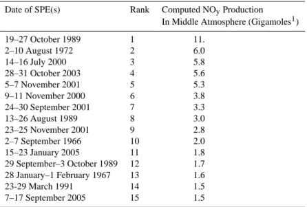
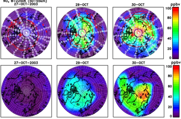
Fig. 4. Top three plots are taken from Fig. 2 of L´opez-Puertas et al. (2005a) and show the Northern Hemisphere polar atmospheric abundance of NOx(ppbv) for days 27, 29, and 30 October 2003,
which is just before and during a major solar proton event at a potential temperature of 2250 K. Contours are zonally smoothed within 700 km. Individual measurements are represented by dia-monds. The polar vortex edge is represented with a red curve and the geomagnetic pole is marked with a red plus sign. The circle around the pole represents the polar night terminator. Bottom three plots are from WACCM3 simulation 4(a) for the same three days at 0.55 hPa (∼55 km).
5.2 NOx(N, NO, NO2)constituents
The NOxspecies have considerably longer lifetimes than the
HOx species and are produced in great abundance during
very large SPEs. For example, we have evidence of huge enhancements of NOxas a result of the “Halloween Storms”
of 2003. The Envisat MIPAS instrument provided simulta-neous observations of NOx in both polar regions. Atomic
nitrogen (N) is quite small in the mesosphere and strato-sphere; thus, the MIPAS measurements of NO and NO2
es-sentially provide a measure of the polar NOxenhancements
during the “Halloween Storms” of 2003. We show the MI-PAS Northern Hemisphere polar NOxon three days (27, 29,
and 30 October) in Fig. 4 (top) at the 2250 K (50–55 km) surface. The polar vortex edge has been calculated using the criteria discussed in Nash et al. (1996) but modified so that a long-lived chemical constituent influenced by dynam-ics (CH4 below 1500 K and CO above) has been used,
in-stead of the mean zonal winds. That is, the vortex edge is de-fined where there coexists a pronounced gradient in potential vorticity and a large gradient in the dynamically-influenced constituent. This vortex boundary is represented with a red curve and the geomagnetic pole is marked with a red plus sign. Some individual NOxvalues reached 180 ppbv, about
a factor of ten larger than normal under unperturbed condi-tions. Generally, the largest average NOxvalues were close
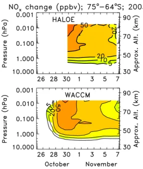
Fig. 5. Top plot is adapted from Fig. 7 of Jackman et al. (2005a) and shows the daily average HALOE sunset-measured polar Southern Hemisphere NOxchange caused by the late October–early
Novem-ber 2003 SPEs beyond the ambient atmosphere amounts measured 12–15 October 2003. The HALOE measurements were at latitudes between 64◦and 75◦S. Bottom plot is derived from WACCM3
sim-ulation 4(a) in a similar way and indicates the NOxchange caused
by the October–November 2003 SPEs beyond the ambient atmo-sphere amounts on 25 October (before the SPEs). Contour levels plotted are 5, 10, 20, 50, and 100 ppbv. The colored region indi-cates statistically significant changes at the 2σ level in the bottom plot.
We present WACCM3 results for the same three days in Fig. 4 (bottom) from simulation 4(a). The model shows sim-ilar qualitative and quantitative behavior with polar NOx
lev-els reaching over 90 ppbv. There are differences in the shape of the SPE-perturbed region, which are probably due to dif-ferences between the transport in WACCM3 and the Earth’s atmosphere at this level. WACCM3 is a free-running climate model, so the computations cannot be expected to reproduce in detail the conditions prevailing in the atmosphere at any particular time.
NOx levels were also measured during this period by
UARS HALOE. We show the excess NOxbeyond baseline
amounts before the SPE period in Fig. 5 (top) (adapted from Fig. 7 of Jackman et al., 2005a). This plot was constructed with HALOE sunset profiles taken at high southern latitudes (64◦ and 75◦S) in the SPE-disturbed period 30 October–7 November 2003 differenced with those sunrise profiles taken at high southern latitudes before the SPE (12–15 October 2003). Since NO and NO2are tightly coupled and the
quan-tity NO+NO2 is highly conserved during a 24-h period in
the upper stratosphere and mesosphere, it is possible to
com-Fig. 6. Temporal evolution of nighttime NO2abundance changes relative to 26 October for the polar Northern Hemisphere (70– 90◦N) from MIPAS with the reprocessed version V3O NO
29 data
(top). Middle plot is derived from WACCM3 simulation 4(a), which includes SPEs, and indicates nighttime NO2changes relative to 25
October in 70–90◦N. The colored areas in the middle plot demon-strate the 2σ statistically significant regions. Bottom plot is derived from WACCM3 simulation 4(w), which does not include SPEs, and indicates NO2seasonal changes relative to 25 October for night in
70–90◦N. Contour levels plotted are –4, –3, –2, –1, 0, 2, 5, 10, 20,
30, 40, 50, 60, 70, 80, and 90 ppbv.
pare sunrise NOxmeasurements with sunset NOx
measure-ments and derive the perturbed atmospheric NOxchanges for
a short period (approximately a week).
We present WACCM3 results from simulation 4(a) for NOx during this same period in Fig. 5 (bottom). The
WACCM3 results are zonal average values over the same latitude band as HALOE. These model/measurement com-parisons are valid because the NOxfamily changes so slowly
with time. The values in the plot show the excess NOx
be-yond the 25 October 2003 levels (quiet period). The colored region indicates 2σ statistically significant changes. Both the observations and the model indicate a very similar tempo-ral structure. Huge NOx increases of greater than 100 ppbv
(red color) were produced in the middle to upper meso-sphere (0.03 to 0.006 hPa) for 30–31 October . The lower mesosphere showed NOxincreases of greater than 20 ppbv
throughout the period, compared with unperturbed values of less than 1 ppbv (Jackman et al., 2005a). There are some modest differences between the WACCM3 predictions and the HALOE measurements. However, given the huge NOx
changes from this perturbation, WACCM3 and HALOE are in reasonable agreement.
The nighttime NH MIPAS NO2 enhancements are
com-pared with WACCM3 results in Fig. 6. The reprocessed MI-PAS version V3O NO29 data are given here. WACCM3
simulation 4(a) (Fig. 6, middle) shows NO2 increases over
90 ppbv and MIPAS (Fig. 6, top) observes maximum NO2
increases of about 70 ppbv in the lower mesosphere. The enhanced NO2 is long-lasting with amounts greater than
30 ppbv in both MIPAS and WACCM3 between 45 and 55 km through 14 November. The downward transport of NO2over this time period is also evident in both MIPAS and
WACCM3. Figure 6 (bottom) shows WACCM3 results from a simulation without SPEs, simulation 4(w), which indicates that the seasonal changes are generally negative at this time of year. The colored areas Fig. 6 (middle) illustrate the re-gions where the perturbation is statistically significant at the 2σ level. For these altitudes nighttime NO2 is essentially
NOx. The WACCM3 results qualitatively agree with MIPAS.
However, WACCM3 is generally larger than MIPAS (usu-ally 15 ppbv or more) at most altitudes above 45 km. From 35–45 km MIPAS mostly measures higher levels of NO2
en-hancement than predicted. Below 35 km both MIPAS and WACCM3 show seasonal NO2decreases.
5.3 Ozone
Ozone was also impacted by these SPEs. The SPE-produced HOxand NOxconstituents led to short- and longer-term
cat-alytic ozone destruction in the lower mesosphere and strato-sphere (pressures greater than about 0.5 hPa). The tempo-ral evolution of changes in ozone abundance measured by MIPAS during and after the October–November 2003 SPEs is given in Fig. 7 (top). These values are presented for the Southern Hemisphere (SH) (70–90◦S) and Northern Hemi-sphere (NH) (70–90◦N) polar caps. The reprocessed MIPAS version V3O O3 9 data are shown here. The measurements
are compared to WACCM3 predictions from simulation 4(a) in the same regions in Fig. 7 (upper middle). Due to the short lifetime of HOxconstituents (see Fig. 3), their ozone
influ-ence lasts only during and for a few hours after the SPEs. This explains the huge measured and modeled ozone deple-tion above 50 km on 29–30 October and, to a lesser extent, on 3–4 November. Note that Fig. 1 shows ion pair production, which is essentially a proxy for the NOxand HOxproduction.
WACCM3 predictions in Fig. 7 (lower middle) are the same as Fig. 7 (upper middle) except the colored areas illustrate the regions where the perturbation is statistically significant at the 2σ level. Figure 7 (bottom) shows WACCM3 results from a simulation without SPEs, simulation 4(w), indicating the seasonal changes at this time of year.
Fig. 7. Top two plots are similar to Fig. 4 of L´opez-Puertas et al. (2005a) but with the reprocessed MIPAS version V3O O3 9
data and show the temporal evolution of changes in ozone relative to 25 October during and after the October–November 2003 SPEs for the Southern Hemisphere (SH) (70–90◦S) (left) and Northern
Hemisphere (NH) (70–90◦N) (right) polar caps. Upper middle two
plots are derived from WACCM3 simulation 4(a) and indicate ozone changes relative to 25 October. Lower middle two plots are the same as the upper middle two plots except the colored areas demonstrate the 2σ statistically significant regions. Bottom plots are derived from WACCM3 simulation 4(w), which does not include SPEs, and indicates ozone seasonal changes relative to 25 October. Contour levels plotted are –70, –65, –60, –55, –50, –45, –40, –35, –30, –25, –20, –15, –10, –5, 0, 5, 10, 20, and 40%.
SPE impacts in the NH are larger than the SH in both mod-els and simulations. NH ozone depletion exceeds 50% dur-ing the SPEs in late October. These interhemispheric dif-ferences in ozone depletion are caused by the difdif-ferences in solar zenith angle between the NH and SH. The NH with the larger solar zenith angle has a larger percentage HOxchange
(see Fig. 3) than the SH and thus a larger short-term impact on ozone (for further discussion see Solomon et al., 1983). Polar NH upper stratospheric ozone depletion greater than 30% continues through 14 November, the end of the plot-ting period. The polar SH shows ozone reduction greater
Fig. 8. Left plot shows NOAA-14 SBUV/2 Northern Hemisphere polar ozone percentage change at 0.5 hPa from 13 July 2000 (before the SPE) to 14–15 July 2000 (maximum proton intensity). Right plot shows WACCM3 “snapshot” using simulation 3(a) of polar ozone percentage change at 0.5 hPa for 00:00 GMT from 13 July to 15 July 2000. The colored areas in the right plot demonstrate the 2σ statistically significant regions.
than 30% during the SPEs in late October with lower meso-spheric ozone depletion from 5–10% continuing through 14 November.
The measured and modeled ozone depletions show some differences. The NH modeled ozone indicates a larger re-covery (ozone enhancement) above ∼57 km after 7 Novem-ber, than indicated in the measurements. This apparent NH ozone recovery is due to seasonal changes (see bottom plots in Fig. 7), wherein ozone is enhanced via transport from above. The SH modeled ozone below ∼45 km indicates a larger ozone depletion after 2 November, than indicated in the measurements. The reason(s) behind these NH and SH model-measurement differences are still unclear, but is prob-ably caused in part by the fact that transport and temperature in WACCM do not correspond to any specific year.
Other measurements of short-term ozone loss caused by solar protons are available for other SPEs. For example, a very large SPE commenced on 14 July 2000, the so-called “Bastille Day” solar storm, which was the third largest SPE period in the past 45 years. This SPE took place over the 14–16 July period. Jackman et al. (2001) showed Northern Hemisphere polar ozone changes (in ppmv) from the NOAA 14 SBUV/2 instrument at 0.5 hPa due to the July 2000 SPE between 13 July (before SPE) and 14–15 July (during SPE), 2000. We provide a similar plot in Fig. 8, which shows the percentage change for ozone from 13 July to 14–15 July for NOAA 14 SBUV/2 and from 13 July to 15 July at 0:00 GMT from the average of WACCM3 simulations 3(a, b, c, d). Fig-ure 8 (left) is constructed from 24 h of NOAA 14 SBUV/2 orbital data during the maximum intensity of the event and Fig. 8 (right) is a difference of model “snapshots.” The col-ored areas in Fig. 8 (right) demonstrate the 2σ statistically significant changes.
The polar cap edge (60◦ geomagnetic latitude), wherein the protons are predicted to interact with the atmosphere, is indicated by the white circle. Large ozone decreases of 30–40% are seen at this pressure level in both the SBUV/2 observations and WACCM3 calculations, which are primar-ily caused by the SPE. These ozone decreases are driven by catalytic destruction from the HOxincreases of ∼100% and
are mostly confined to the polar cap areas (e.g. Jackman et al., 2001). The polar cap changes are nearly all statistically significant at 2σ . Overall there is good agreement between WACCM3 and SBUV/2.
5.4 Other constituents
Several other constituents appear to have been influenced as a result of the SPEs during the “Halloween Storms” of 2003, including HNO3, N2O5, ClONO2, HOCl, and ClO (Orsolini
et al., 2005; von Clarmann et al., 2005; L´opez-Puertas et al., 2005b). Here we show WACCM3 comparisons with all of these constituents.
5.4.1 HNO3change
Figure 9 (top) shows the temporal change in Envisat MIPAS V3O HNO3 9 measurements of HNO3 during the
night-time in the polar Northern Hemisphere (70–90◦N). L´opez-Puertas et al. (2005b) argued that the observed HNO3
in-creases in the upper stratosphere and lower mesosphere were probably primarily caused by the gas-phase reaction, NO2+OH+M→HNO3+M. Both OH and NO2enhancements
were simulated when WACCM3 was run with SPEs and the inclusion of this reaction in WACCM3 led to increases in HNO3.
We show WACCM3 results in Fig. 9 for two types of rep-resentation: 1) usual representation on the model grid, called WACCM; and 2) after application of the MIPAS averaging kernel (AK), called WACCM (AK). This second represen-tation can significantly change the model results for con-stituents HNO3, N2O5, ClONO2, HOCl, and ClO, but is
of minor influence on the WACCM3/MIPAS ozone compar-isons (Fig. 7). MIPAS retrievals are based on constrained least squares fitting of modeled to measured spectra (von Clarmann et al., 2003). The applied constraint smooths the vertical profiles and affects the retrieval particularly at alti-tudes where MIPAS is not very sensitive to the emission of the particular constituent. The model and MIPAS data are more comparable when the MIPAS AKs are applied to the WACCM data (Rodgers, 2000). The result WACCM (AK) is what MIPAS would see if it would sound the atmospheric state as modeled by WACCM.
The usual representation of model results from simula-tion 4(a) (see Fig. 9, middle left) suggest that HNO3
in-creases were largest above 45 km and below 30 km in the period plotted. The sampling of simulation 4(a) results with the MIPAS AK moves the peak of the HNO3 increases to
a lower altitude (by a few km), reduces the peak amounts, and does not significantly improve the model/measurement agreement. The colored areas in Fig. 9 (middle plots) illustrate the regions where the perturbation simulated in WACCM3 is statistically significant at the 2σ level. Fig-ure 9 (bottom plots) shows WACCM3 results from a simu-lation without SPEs, simusimu-lation 4(w), which indicates that there are seasonal changes, but none that are very important above 35 km.
It is difficult to understand the large observed changes in the 35–55 km altitude range which are not simulated in WACCM3, given the ionization rates of Fig. 1, without involving some other pathway for HNO3production such as
ion chemistry. L´opez-Puertas et al. (2005b) discussed the following ion chemistry scheme for HNO3production:
O+2H2O+H2O → H3O+·OH+O2
H3O+·OH+H2O → H+·(H2O)2+OH
H+·(H
2O)2+NO−3 →HNO3+H2O+H2O
Net : H2O+NO3→HNO3+OH
This pathway for HNO3 production, first proposed by
Solomon et al. (1981), requires the production of NO−3 and functions under dark conditions. Although ion chemistry in-volving N+2, O+2, N+, NO+, O+, and electrons is included in WACCM3, ion reactions involving water are presently not included. It is beyond the scope of this paper to include such a water cluster ion scheme for HNO3 production. Another
possible reason behind the model/measurement discrepancy could be a faster reaction rate for NO2+OH+M→HNO3+M
than was given in Sander et al. (2003) and employed in WACCM3.
The enhanced HNO3measured by MIPAS during the peak
of the solar event is rather temporary with a peak over 2.5 ppbv on 29–31 October 2003 between 42 and 50 km de-creasing rapidly to less than 0.4 ppbv by 8 November 2003 and increasing again to greater than 0.8 ppbv by 15 Novem-ber 2003. Although the latter MIPAS HNO3enhancement
(between 8 and 15 November) is still somewhat different from the WACCM3 predictions, both observations and model prediction show relatively slow HNO3 changes over this
week period (8–15 November). 5.4.2 N2O5change
Envisat MIPAS V3O N2O5 9 measurements and WACCM3
computations of N2O5are presented for the polar Northern
Hemisphere (70–90◦N) in Fig. 10. The temporal change in Envisat MIPAS N2O5 during the nighttime in the polar
Northern Hemisphere (70–90◦N), shown in Fig. 10 (top), is fairly similar to that given in Fig. 5 of L´opez-Puertas et
Fig. 9. Top plot is similar to Fig. 2a of L´opez-Puertas et al. (2005b) but with the reprocessed version V3O HNO39 data and shows the temporal evolution of MIPAS HNO3abundance changes relative to
26 October for nighttime in the polar Northern Hemisphere (70– 90◦N). Middle plots are derived from WACCM3 simulation 4(a), which includes SPEs, and indicate HNO3 changes relative to 25
October. The colored areas in the middle plots demonstrate the 2σ statistically significant regions. Bottom plots are derived from WACCM3 simulation 4(w), which does not include SPEs, and in-dicates HNO3seasonal changes relative to 25 October. Middle and
bottom plots indicate usual sampling of the model [WACCM] and MIPAS averaging kernel applied to the WACCM results [WACCM (AK)]. Contour levels plotted are –0.6, –0.4, –0.2, 0.0, 0.2, 0.4, 0.6, 0.8, 1.0, 1.2, 1.4, 1.6, 1.8, 2.0, 2.5, and 3.0 ppbv.
al. (2005b) even though the reprocessed level-1b data and re-vised retrieval control parameters were used.
The usual sampling of model results from simulation 4(a) (see Fig. 10, middle left) show that N2O5modeled
enhance-ments peaked at about 45 km near the last day plotted (14 November), about 5 km higher than the MIPAS peak. Also, WACCM3 predicted N2O5increases of 5–6 ppbv (primarily
driven by the SPEs) in Fig. 10 (middle left) were significantly larger than the MIPAS measured increases of about 1 ppbv. The sampling of simulation 4(a) results with the MIPAS AK moves the peak of the N2O5increases to about 40 km, in
bet-ter agreement with MIPAS. However, the predicted increases are still significantly higher than MIPAS with peak levels at about 4–5 ppbv. The colored areas in Fig. 10 (middle plots)
Fig. 10. Top plot is similar to Fig. 5 of L´opez-Puertas et al. (2005b) but with the reprocessed version V3O N2O59 data and shows the
temporal evolution of MIPAS N2O5abundance changes relative to 26 October for nighttime in the polar Northern Hemisphere (70– 90◦N). Middle plots are derived from WACCM3 simulation 4(a)
and indicate N2O5 changes relative to 25 October for night in
70–90◦N. The colored areas in the middle plots demonstrate the
2σ statistically significant regions. Bottom plots are derived from WACCM3 simulation 4(w) and indicate N2O5seasonal changes
rel-ative to 25 October. Middle and bottom plots indicate usual sam-pling of the model [WACCM] and MIPAS averaging kernel applied to the WACCM results [WACCM (AK)]. Contour levels plotted are –0.6, –0.4, –0.2, –0.1, –0.05, 0.0, 0.05, 0.1, 0.15, 0.2, 0.25, 0.3, 0.35, 0.4, 0.6, 0.8, 1.0, 1.5, 2, 3, 4, 5, and 6 ppbv.
illustrate the regions where the perturbation is statistically significant at the 2σ level.
WACCM3 predicted seasonal changes in N2O5are shown
in Fig. 10 (bottom plots) from a computation without SPEs [simulation 4(w)]. These plots indicate the importance of the seasonal changes in forcing the N2O5 enhancement of
0.6 ppbv between 29 and 33 km from 26–31 October 2003. The seasonal changes contribute somewhat to the N2O5
in-creases in the mid- to upper stratosphere (30–50 km) in November 2003 for both the usual sampling and the MIPAS AK sampling of the model results.
The cause of the discrepancy between the model and mea-surements at these altitudes could be related to the speed at
which N2O5is produced via
NO2+NO3+M → N2O5+M.
For example, if this reaction proceeds much slower than indi-cated in Sander et al. (2003), then the build-up of N2O5will
be reduced after a large solar event. Conversely, the thermal decomposition reaction
N2O5+M → NO2+NO3+M
and/or the photodissociation of N2O5 may be proceeding
more rapidly than indicated in Sander et al. (2003), prevent-ing a larger build-up of N2O5after a large solar event. At the
present time, it is impossible to determine what reaction(s) need to be corrected in WACCM3 to simulate better agree-ment with MIPAS. Also, the production of N2O5is very
sen-sitive to the temperature and dynamics. Differences between the predicted/real temperatures and/or differences in the dy-namics (downward transport of earlier-produced NO2)might
explain some of these differences. 5.4.3 ClONO2change
We show Envisat MIPAS V3O ClONO2 9 measurements
and WACCM3 computations of ClONO2in Fig. 11 for the
polar Northern Hemisphere (70–90◦N). The MIPAS obser-vations showed ClONO2 maximum enhancements at 35–
40 km of 0.3–0.4 ppbv starting right after the largest proton fluxes on 29–30 October (Fig. 11, top). The usual representa-tion of model results from simularepresenta-tion 4(a) (see Fig. 11, mid-dle left) show predicted ClONO2increases at approximately
the same amounts, however, the peak production was at a higher altitude (40-45 km) and several days later than mea-sured.
The sampling of simulation 4(a) results with the MIPAS AK moves the peak of the ClONO2increases to about 40 km,
in better agreement with MIPAS. However, the predicted peak increases are reduced substantially to about 0.2 ppbv, about a factor of two less than observed. The colored areas in Fig. 11 (middle plots) illustrate the regions where the per-turbation is statistically significant at the 2σ level.
The SPE-produced NOxleads to enhanced ClONO2
pro-duction via
ClO+NO2+M → ClONO2+M.
The cause of the discrepancy between the model and mea-surements at these altitudes could be related to the speed of this reaction. If this reaction proceeds much faster than indi-cated in Sander et al. (2003), then the build-up of ClONO2
will be enhanced to larger amounts more quickly after a large solar event. However, any changes in the rate for this reac-tion will also impact the ClO amounts (discussed below) and need to be considered carefully. Predicted seasonal changes (Fig. 11, bottom) mostly indicated increases over the time period although they appear to be primarily important below 35 km.
Fig. 11. Top plot is similar to Fig. 1 (bottom) of von Clarmann et al. (2005) and Fig. 8 of L´opez-Puertas et al. (2005b) but with the reprocessed version V3O ClONO29 data and shows the
tem-poral evolution of MIPAS ClONO2abundance changes relative to 26 October for nighttime in the polar Northern Hemisphere (70– 90◦N). Middle plots are derived from WACCM3 simulation 4(a)
and indicate ClONO2seasonal changes relative to 25 October. The
colored areas in the middle plot demonstrate the 2σ statistically sig-nificant regions. Bottom plots are derived from WACCM3 simula-tion 4(w) indicates ClONO2seasonal changes relative to 25
Octo-ber. Middle and bottom plots indicate usual sampling of the model [WACCM] and MIPAS averaging kernel applied to the WACCM re-sults [WACCM (AK)]. Contour levels plotted are –0.05, 0.0, 0.05, 0.1, 0.15, 0.2, 0.25, 0.3, 0.35, and 0.4 ppbv.
5.4.4 HOCl change
Envisat MIPAS V2 HOCl 1 measurements and WACCM3 computations of HOCl simulation 4(a) are presented for the polar Northern Hemisphere (70–90◦N) in the top and bot-tom of Fig. 12, respectively. The measurements show sig-nificant HOCl enhancements in the altitude range 30–55 km. The mechanism for increasing HOCl as a result of the SPEs involves enhancing the HOx constituents, which then speed
up the following gas-phase three reaction sequence: OH+HCl → H2O+Cl
Cl+O3→ClO+O2
ClO+HO2→HOCl+O2.
Fig. 12. Top plot is adapted from Fig. 1 (middle) of von Clarmann et al. (2005) and shows the temporal evolution of MIPAS V2 HOCl 1 measurements of HOCl changes relative to 26 October for nighttime in the polar Northern Hemisphere (70–90◦N). Bottom plot is
de-rived from WACCM3 simulation 4(a) and indicates HOCl changes relative to 25 October. The colored areas in the bottom plots demon-strate the 2σ statistically significant regions. Bottom plots indicate usual sampling of the model [WACCM] and MIPAS averaging ker-nel applied to the WACCM results [WACCM (AK)]. Contour levels plotted range from –0.05 to 0.5 ppbv with an interval of 0.05..
The usual representation of model results from simula-tion 4(a) (see Fig. 12, bottom left) show WACCM3 predicted HOCl increases from 35 km up to 60 km and above. The modeled peak enhancement is about 0.2–0.25 ppbv larger than measured. WACCM3 results also show a secondary HOCl peak on 4 November due to a smaller SPE in this pe-riod (Fig. 1).
The application of the MIPAS averaging kernels to the simulation 4(a) results moves the peak of the HOCl increases to the altitude range 30–55 km and totally eliminates the sec-ondary HOCl peak, in better agreement with MIPAS. The predicted peak increases are reduced substantially and now are only about 0.1 ppbv larger than observed. The colored areas in Fig. 12 (bottom plots) illustrate the regions where the perturbation is statistically significant at the 2σ level.
We also investigated model predictions in the WACCM3 computation without SPEs [simulation 4(w), not shown] and found very small seasonal changes over this period, imply-ing that practically all of the measured and modeled HOCl changes were due to the SPEs.
5.4.5 ClO change
ClO is closely coupled to HOCl and ClONO2. We show
Envisat MIPAS V3O ClO 11 measurements and WACCM3 computations of ClO in Fig. 13 for the polar Northern
Fig. 13. Top plot is similar to Fig. 1 (top) of von Clar-mann et al. (2005) and shows the temporal evolution of MIPAS V3O ClO 11 measurement of ClO changes relative to 26 October for nighttime in the polar Northern Hemisphere (60–80◦N). Middle
plots are derived from WACCM3 simulation 4(a) and indicate ClO changes relative to 25 October. The colored areas in the middle plot demonstrate the 2σ statistically significant regions. Bottom plots are derived from WACCM3 simulation 4(w) indicate ClO seasonal changes relative to 25 October. Middle and bottom plots indicate usual sampling of the model [WACCM] and MIPAS averaging ker-nel applied to the WACCM results [WACCM (AK)]. Contour levels plotted range from –0.35 up to 0.45 ppbv with an interval of 0.05.
Hemisphere (60–80◦N). MIPAS provides better ClO mea-surements in this latitude band than that used for the other constituents in this section (i.e., 70–90◦N). Generally, the MIPAS observations show ClO enhancements in the 30– 50 km altitude range, peaking over 0.2 ppbv on three sepa-rate days (30 Oct, 1 Nov, and 8 Nov), although there are two days (4 and 10 Nov) when decreases are measured. The usual representation of model results from simulation 4(a) (see Fig. 13, middle left) show predicted ClO increases only above 55 km and then only for about 3 days (28–31 Oct). Between 40 and 55 km, the WACCM3 ClO shows a de-crease throughout the time period with peak reductions over 0.3 ppbv.
The application of the MIPAS averaging kernels to the simulation 4(a) results moves the decreases in ClO to lower altitudes and diminishes the peak ClO reductions to
∼0.15 ppbv. The colored areas in Fig. 13 (middle plots)
il-lustrate the regions where the perturbation is statistically sig-nificant at the 2σ level. Predicted seasonal changes (Fig. 13, bottom) mostly indicated decreases over the time period that are about 1/3 to 1/2 of the computed changes occurring at this time of year.
The production of ClO during SPEs was discussed in von Clarmann et al. (2005). SPE-produced OH can release reactive chlorine (Cl) from the reservoir HCl (OH+HCl→H2O+Cl) and lead to the creation of ClO
(Cl+O3→ClO+O2). Loss of ClO during SPEs is also
pos-sible through the SPE-produced HO2(HOx) and NO2(NOx)
creating HOCl and ClONO2via the reactions ClO+HO2→
HOCl+O2and ClO+NO2+M → ClONO2+M.
The reasons behind the significant differences between MIPAS and WACCM3 ClO are presently not known. A study with a simpler model, which would allow easier addition or subtraction of included reactions and/or modifications in re-action rates, would be helpful in elucidating the major causes of these discrepancies.
6 SPE-induced medium-term (months) changes in com-position
Very large SPEs produced NOxin the polar mesosphere and
upper stratosphere (Zadorozhny et al., 1992; Jackman et al., 2001, 2005; L´opez-Puertas et al., 2005b). These NOx
pertur-bations were significantly reduced in the sunlit hemisphere through the two step process [NO+hν→N+O followed by N+NO→N2+O]. However, the SPE-caused NOx
enhance-ments in the darker hemisphere had a very long lifetime (∼months) and ended up being transported to the middle and lower stratosphere. This increased NOx had associated
ozone decreases over its lifetime. We will discuss this pro-cess following the very large SPEs of July 2000 and October 1989 and show measurements and model simulations for 2– 5 months past these SPEs. We will also show evidence of longer lasting (∼two months) SPE-caused ozone depletion following the August 1972 SPEs, likely caused by the SPE-produced NOxenhancements.
6.1 July 2000 Solar Proton Event
The July 2000 SPE produced large amounts of NOx, which
was observed by HALOE and simulated in a 2-D model (Jackman et al., 2001). We computed an ensemble aver-age of the two groups of simulations 3(a, b, c, d) and 3(w, x, y, z) and differenced the two to derive the results shown in Fig. 14. Note the near anti-correlation of NOx (Fig. 14,
left) and ozone (Fig. 14, right) over most of this period. The HOx constituents (not shown) produced during the SPE on
days 196–198 (14–16 July) are responsible for the short-lived large ozone decreases (>40%). The SPE-caused NOx
en-hancement then drives the ozone depletion after this period. This is consistent with the downwelling associated with the
Fig. 14. Derived from WACCM3 output showing the difference of the ensemble average of simulations 3(a, b, c, d) compared to the ensemble average of simulations 3(w, x, y, z) for the latitude band 60–90◦S from day 195 (13 July) through day 275 (1 October)
for year 2000. Top left plot indicates NOx change with contour
levels of 0, 5, 10, 15, 20, 30, 40, 60, 80, and 100 ppbv. Top right plot indicates ozone change with contour levels of –40, –30, –20, –15, –10, –5, 0, and 5%. Bottom plots are the top plots repeated with the colored areas indicating the regions which are statistically significant at the 2σ level for NOxand ozone.
residual circulation over the SH polar regions during July. By about day 255 (11 September), a NOx increase of >5 ppbv
appears to cause an ozone loss of >10%. The rate of de-scent of the NOxand ozone perturbation is about 140 m/day
(∼0.16 cm/s) over this period consistent with the residual cir-culation velocities during this time. Near the end of the plot-ted period (day 274), predicplot-ted NOx enhancements greater
than about 4 ppbv and ozone decreases greater than about 20% are statistically significant at 2σ , which are indicated by the colored areas in the bottom plots in Fig. 14.
Is there any evidence of SPE-caused NOxenhancements
lasting at least six weeks after the event period, as simu-lated by WACCM3? Yes: Randall et al. (2001) showed ev-idence from HALOE observations of large NOx(NO+NO2)
enhancements two months after this July 2000 SPE in the Southern Hemisphere. Ten years of HALOE observations are presented in Fig. 15 (left). Although there is evidence of interannual variability, the year 2000 shows enhancements of NOxby about a factor of 2–3 beyond the normal range near
1000 K (∼33 km).
We have sampled the WACCM3 output of simulation 1(a) in a similar manner and present the results in Fig. 15 (right). The WACCM3 results indicate somewhat larger interannual variability above about 32 km, and less variability below this altitude. Both HALOE and WACCM3 show NOx
enhance-ments in year 2000 greater than 10 ppbv beyond the normal range. NOx changes greater than about 4 ppbv are
statisti-cally significant at the 2σ level throughout this altitude range at this time of year. Thus the July 2000 SPE likely led to these September 2000 NOxincreases.
Fig. 15. Left plot is an adaptation of Fig. 5a of Randall et al. (2001) showing Southern Hemisphere (SH) polar vortex HALOE NOx
(ppbv) profiles in September/October for years 1991–2000. Right plot shows WACCM3 simulation 1(a) predicted SH polar vortex NOx(ppbv) profiles for the same periods.
The sharper peak in WACCM3 is likely related to the coarser altitude grid in the model. There are differences in the interannual variability in WACCM3 compared with HALOE near the top level shown (1500 K, ∼40 km) in Fig. 15. The cause of these differences in the upper strato-sphere between WACCM3 and HALOE may be related to A) a larger production in WACCM3 of lower thermospheric NOxvia auroral electrons than exists in the atmosphere; B)
a larger downward transport in WACCM3 of NOxfrom the
lower thermosphere to the stratosphere; C) a combination of A) and B); or D) other differences between WACCM3 and the atmosphere. It is unclear what the differences in the lower stratosphere between WACCM3 and HALOE mean. A strong possibility is that there are different dynamics in the model and actual atmosphere. For instance, the local maxima near 700–800 K in the HALOE data likely result from downward transport of NOx produced earlier in the
winter at higher altitudes by energetic particle precipitation (see Randall et al., 2007); WACCM3 might not be simulat-ing this transport adequately. Recall that since the version of WACCM3 used here is not forced by analyzed winds, we do not expect the model dynamics to match the atmospheric dynamics in detail for any specific year.
6.2 August 1972 Solar Proton Events
The second largest SPE period in the past 45 years oc-curred 2–10 August 1972 (days 215–223). Although this SPE period occurred about 35 years ago, there were recorded measurements of its ozone impact (e.g. Heath et al., 1977; Reagan et al., 1981; McPeters et al., 1981; Jackman and McPeters, 1987; Jackman et al., 1990). We compare our WACCM3 predicted ozone changes to measured ozone changes from the backscattered ultraviolet (BUV) instrument on the Nimbus 4 satellite between about 32 and 53 km for 60 days in Fig. 16. The BUV changes (Fig. 16a) were de-rived by comparing 1972 to 1970 ozone data (Jackman et al.,
Fig. 16. Plot (a) is taken from Fig. 6 of Jackman et al. (1990) and shows the temporal evolution of measured ozone abundance changes in 1972 relative to 1970 by the backscattered ultraviolet (BUV) instrument aboard the Nimbus 4 satellite for the latitude band 70–80◦N. Plot (b) is derived from the WACCM3 ensemble average of simulations 1(a, b, c, d) and indicates ozone changes in 1972 relative to 1970 in the same latitude bands. The shaded area in plot (b) demonstrates the 2σ statistically significant region. Con-tour levels plotted are –30, –20, –15, –10, –5, and 0%.
1990) in latitude band 70–80◦N. The WACCM3 computed ozone changes (Fig. 16b) were derived by averaging the en-semble of simulations 1(a, b, c, d) and comparing 1972 to 1970 for the same latitude band. The shaded area in Fig. 16b illustrate the regions where the perturbation is statistically significant at the 2σ level.
There is reasonable agreement between the model and measurement with both showing significant ozone depletion (>10%) in the upper stratosphere (∼40–50 km) over most of the 60-day time period in the 70–80◦N latitude band. Both model and measurement show modest ozone depletion (5– 10%) in the altitude region 40–45 km over most of the pe-riod in the 50–60◦N latitude band (not shown). Also, the measurements indicate a larger ozone depletion in the 33– 40 km region for both latitude bands than simulated by the model. As explained in Jackman et al. (2000), only proton
Fig. 17. Temporal evolution of WACCM3-computed percentage ozone change in 1989 for the ensemble average of simulations 2(a, b, c, d) average compared to the ensemble average of simula-tions 2(w, x, y, z) at 70◦N for NO2(top left) and Ozone (top right).
Contour levels for NO2are –40, –20, –10, 0, 10, 20, 40, 70, 100,
and 1000%. Contour levels for Ozone are –20, –15, –10, –5, 0, 5, 10, and 15%. Bottom plots are the top plots repeated with the col-ored areas indicating the regions which are statistically significant at the 2σ level for NO2and ozone.
fluxes with energies less than 100 MeV were included for these SPEs. The August 1972 events probably had protons with energies greater than 100 MeV, which affect altitudes below 35 km. These high-energy protons, however, could not be reliably included into our computations.
6.3 October 1989 Solar Proton Events
The largest SPE period in the past 45 years occurred 19–27 October (Days 292–300), 1989. The NOyproduced during
this period was nearly a factor of two larger than the second largest SPE period (see Table 1). Both rocket measurements (NO; Zadorozhny et al., 1992) and satellite measurements (ozone and NO2; Jackman et al., 1993, 1995) showed
atmo-spheric changes as a result of these extremely intense SPEs. We computed an ensemble average of the two groups of simulations 2(a, b, c, d) and 2(w, x, y, z) and differenced the two to derive the percentage change shown for NO2(Fig. 17,
left) and ozone (Fig. 17, right) at 70◦N. Very large upper stratospheric enhancements of NO2greater than 100% from
late October to early December drive ozone decreases greater than 20%. The substantial ozone depletion (>10%) between 2 and 4 hPa before the 19–27 October SPE period was mainly caused by prior large SPE periods in 13–26 August 1989 and 29 September–3 October 1989 (see Table 1), which produced sufficient NOxto cause a longer-lived ozone loss. The NO2
enhancement in March 1990 was caused by a medium sized SPE (Fig. 17, left). No associated short-term ozone loss by HOxconstituents is seen in Fig. 17 (right) because WACCM3
output was only every five days for these simulations and the SPE’s influence on mesospheric and upper stratospheric ozone on 19–20 March 1990 was missed.