HAL Id: hal-01384457
https://hal.archives-ouvertes.fr/hal-01384457
Submitted on 19 Oct 2016HAL is a multi-disciplinary open access
archive for the deposit and dissemination of sci-entific research documents, whether they are pub-lished or not. The documents may come from teaching and research institutions in France or abroad, or from public or private research centers.
L’archive ouverte pluridisciplinaire HAL, est destinée au dépôt et à la diffusion de documents scientifiques de niveau recherche, publiés ou non, émanant des établissements d’enseignement et de recherche français ou étrangers, des laboratoires publics ou privés.
The improvement of soil thermodynamics and its effects
on land surface meteorology in the IPSL climate model
F. Wang, F. Cheruy, J.-L. Dufresne
To cite this version:
F. Wang, F. Cheruy, J.-L. Dufresne. The improvement of soil thermodynamics and its effects on land surface meteorology in the IPSL climate model. Geoscientific Model Development Discussions, Copernicus Publ, 2016, 9 (1), pp.363 - 381. �10.5194/gmd-9-363-2016�. �hal-01384457�
The improvement of soil thermodynamics and its effects on
1land surface meteorology in the IPSL climate model
23
Fuxing WANG1, *, Frédérique CHERUY1, and Jean-Louis DUFRESNE1
4
1Laboratoire de Météorologie Dynamique du CNRS, Tour 45-55, 3ème étage, 5
Case Postale 99, 4 place Jussieu, 75252 Paris Cedex 05, France
6 7
Abstract
8
This paper describes the implementation of an improved soil thermodynamics in
9
the hydrological module of Earth System Model (ESM) developed at the Institut
10
Pierre Simon Laplace (IPSL) and its effects on land surface meteorology in the IPSL
11
climate model. A common vertical discretization scheme for the soil moisture and for
12
the soil temperature is adopted. In addition to the heat conduction process, the heat
13
transported by liquid water into the soil is modeled. The thermal conductivity and the
14
heat capacity are parameterized as a function of the soil moisture and the texture.
15
Preliminary tests are performed in an idealized 1D framework and the full model is
16
then evaluated in the coupled land/atmospheric module of the IPSL ESM. A nudging
17
approach is used in order to avoid the time-consuming long-term simulations required
18
to account for the natural variability of the climate. Thanks to this nudging approach,
19
the effects of the modified parameterizations can be modeled. The dependence of the
20
soil thermal properties on moisture and texture lead to the most significant changes in
21
the surface energy budget and in the surface temperature, with the strongest effects on
22
the surface energy budget taking place over dry areas and during the night. This has
23
important consequences on the mean surface temperature over dry areas and during
24
the night and on its short-term variability. The parameterization of the soil thermal
25
properties could therefore explain some of the temperature biases and part of the
26
dispersion over dry areas in simulations of extreme events such as heat waves in
27
state-of-the-art climate models.
28 29
2 1 Introduction
1
The soil thermodynamics implemented in the Land Surface Models (LSM) partly
2
controls the energy budget at the land surface. Most of the LSM rely on the resolution
3
of a Fourier Law of diffusion equation for heat with a zero flux condition at a limited
4
soil depth and use classical numerical methods to solve it (Lawrence et al., 2011;
5
Ekici et al., 2014). However, differences are identified in adopted soil depth, in the
6
vertical discretization of the numerical schemes, in the additional physical processes
7
other than heat diffusion taken into account and in the degree of complexity of the
8
parameterization of thermal properties.
9
Several studies investigated the effect of the bottom boundary depth of LSM on
10
the evolution of the subsurface temperature (e.g., Lynch-Stieglitz, 1994; Stevens et al.,
11
2007). Sun and Zhang (2004) suggested that at least 6-15 m depth is required to
12
simulate the temperature annual cycle. However, the location of the lower boundary in
13
LSM used in climate models and describing identical heat transfer processes ranges
14
from 2 m to 10 m (Anderson et al., 2004; Table 1).
15
The heat transfer into the soil results from both heat conduction and heat
16
transport by liquid water (e.g., Saito et al., 2006). The heat transported by liquid water
17
can modify the temperature at the surface and below (e.g., Gao et al., 2003, 2008) but
18
this latter process is often neglected in LSM. Several studies investigated the
19
influence of this process on the land-surface parameters based on 1D experiments
20
based on site observations (e.g., Kollet et al., 2009). However, to our knowledge, the
21
impact of the heat convection has never been evaluated on the global scale.
22
The soil thermal conductivity and the soil heat capacity control the evolution of
23
the subsurface temperature and the energy exchanges between the atmosphere
24
boundary layer and the land surface. Besides water content, the soil thermal properties
25
are affected by many factors such as soil types, soil porosity, and dry density
26
(Peters-Lidard et al., 1998; Lawrence and Slater, 2008). The level of complexity of the
27
parameterization of the thermal properties in state-of-the-art LSM is highly variable
28
(e.g., Balsamo et al., 2009; Gouttevin et al., 2012). Moreover, whereas the soil heat
transfer and the moisture diffusion are coupled through the moisture dependence of
1
the thermal properties, the equations of the soil heat transfer and those of moisture
2
diffusion are often solved on different grids. This choice, made for numerical reasons,
3
can lead to energy conservation issues and a unified vertical discretization might be
4
more appropriate.
5
This paper describes the implementation of an improved soil thermodynamics in
6
the Organizing Carbon and Hydrology In Dynamic EcosystEms (ORCHIDEE;
7
Krinner et al., 2005) LSM. The following issues are addressed: (1) the implementation
8
of the same vertical discretization scheme for soil moisture and soil temperature in
9
climate models; (2) the coupling of soil heat convection by liquid water transfer with
10
soil heat conduction process; (3) the parameterization of the thermal conductivity and
11
heat capacity as a function of soil moisture and texture; (4) the sensitivity of the
12
relevant near surface climate variables simulated by a coupled land/atmospheric
13
model to the soil vertical discretization, the soil heat convection processes and to the
14
soil thermal properties. The ORCHIDEE LSM is coupled to the atmospheric model
15
LMDZ (developed at the Laboratoire de Météorologie Dynamique), which physical
16
parameterizations are described in Hourdin et al. (2013) and in Rio et al. (2013).
17
LMDZOR refers to the atmosphere-land component of the Institute Pierre Simon
18
Laplace Climate Model (IPSL-CM; Dufresne et al., 2013). In the standard version of
19
ORCHIDEE, the soil heat transfer is solved with a classical 1D soil heat conduction
20
approach (Hourdin, 1992). The soil heat convection in ORCHIDEE is neglected. The
21
vertical grid for temperature and moisture are different; the soil depth for the
22
temperature is 5 m with 7 layers (5M7L hereafter) and 2 m for the moisture with 11
23
layers (2M11L hereafter). The moisture profile must therefore be interpolated when
24
diagnosing the soil-moisture-dependent soil thermal conductivity and the soil heat
25
capacity in order to solve the soil heat transfer equation.
26
The new developments for the soil thermodynamics, the soil heat
27
conduction-convection model, its boundary conditions, the choice of the soil depth
28
and the vertical grid are described in Section 2. Land-Surface/Atmosphere coupled
4
sensitivity experiments are performed with the full 3D LMDZOR model and analyzed
1
in Section 3 to evaluate the impact of the new developments for the soil
2
thermodynamics on the global scale. The impact of the soil thermodynamics on the
3
global mean surface temperature and on the short-term temperature variability are
4
discussed in Section 4. Conclusions are drawn in Section 5.
5 6
2 The soil thermodynamics model
7
2.1 Model description
8
The governing equation for heat conduction coupled with the energy transferred
9
by liquid water transport in the soil is described by the following energy conservation
10
equation (Saito et al., 2006):
11
, , 1
where CP and CW are volumetric heat capacities (Jm-3K-1) of moist soil and liquid
12
water, respectively; θ is the volumetric soil moisture (m3m-3); st stands for the soil
13
texture; T is the soil temperature (K); t is the time (s); z is the soil depth (m); λ is the
14
soil thermal conductivity (Jm-1s-1K-1); qL is the flux density of liquid water (ms-1);
15
CWST represents a sink of energy associated with the root water uptake that can be
16
neglected for bare soil (i.e. without any plant); and S is the transpiration amount per
17
second (m-3m-3s-1).
18
Equation (1) is solved using an implicit Finite Difference Method (FDM) with
19
zero heat flux condition at the lower boundary of LSM (see Appendix A1; Hourdin,
20
1992). The bedrock effects in deep soil are not parameterized. At the surface, the
21
energy budget equation is:
22
2
where G1 is the soil heat flux due to heat conduction process; H1 is the sensible heat 1
flux of rainfall due to the difference of temperature between the rainwater and the soil
2
surface (Kollet et al., 2009); Train and TS are the temperature of the rainfall and the soil
3
surface, respectively (K); qL,0 is the infiltrated water flux (ms-1); Frad, , and
4
are the net radiation, sensible heat and latent heat flux respectively (Wm-2); CS is the
5
‘layer’ heat capacity per unit area (Jm-2K-1) and is related to the thickness of the first
6
soil layer. Train is the estimated by wet bulb temperature (Gosnell et al., 1995).
7
The unsaturated soil water flow is described by the 1D Fokker-Planck equation
8
obtained by combining the equation of motion (i.e. Darcy law applied to unsaturated
9
1D ground water flow in an isotropic and homogeneous soil) with the mass balance
10
equation (de Rosnay et al., 2000):
11
, , , , 4
, ,
5 where K(θ) and D(θ) are the hydraulic conductivity (ms-1) and diffusivity (m2s-1),
12
respectively.
13 14
2.2 The parameterization of soil thermal properties
15
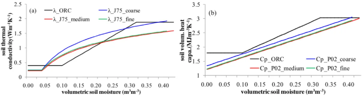
λ and CP are parameterized as a function of moisture and texture (Fig. 1). CP is
16
computed as the sum of heat capacities of soil and water (de Vries, 1963; Yang and
17
Koike, 2005; Abu-Hamdeh, 2003),
18
, , ∆ , 6
where Cv,d and Cv,w are the volumetric heat capacity for dry soil and water (Jm-3K-1),
19
respectively; W is the total water content in the soil layer (m); Δz is the thickness of
20
the soil layer (m), and Cv,d is prescribed and taken from Pielke (2002) (P02, Table 2).
21
There are many ways to compute the soil thermal conductivity, including the
22
method proposed by Johansen (1975, J75 hereafter) recommended by many studies
6
(e.g., Peters-Lidard et al., 1998). Here, the soil freezing process is neglected. The
1
equation for the soil thermal conductivity is given by:
2
λ , 0.7 log 1.0 λ λ λ 7
λ 0.135 1 2700 64.7
2700 0.947 1 2700 8
λ λ λ λ 9
where λdry and λsat are the dry and saturated thermal conductivity, respectively
3
(Wm-1K-1); λw, λq and λo are the thermal conductivity of water, quartz and other
4
minerals, respectively (Wm-1K-1); np is the soil porosity; and q is the quartz content.
5
The variables np and q depend on the soil texture (Table 2). The soil thermal
6
conductivity at the layer interface is linearly interpolated according to the thickness of
7
the layers using the soil thermal conductivity at the nodes where the soil moisture is
8
computed.
9
The soil thermal inertia (I, Wm-2K-1·s0.5) and the soil heat diffusivity (KT, m2s-1)
10
are introduced to help interpreting the results. The soil thermal inertia measures the
11
resistance of the soil to a temperature change induced by an external periodic forcing.
12
The higher I is, the slower the temperature varies during a full heating/cooling cycle
13
(e.g., 24-hour day). KT depicts the ability of the soil to diffuse heat. The larger KT is,
14
the more rapidly the heat diffuses into the ground.
15
, , , 10
, ,
, 11
16
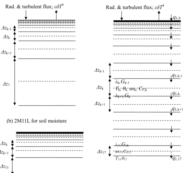
2.3 The vertical discretization in the soil thermodynamics model
17
A common vertical discretization for the soil moisture and for the soil
18
temperature is proposed (Fig. 2c). Using this discretization, the soil moisture profile
does not need to be interpolated in order to diagnose the moisture-dependent thermal
1
properties when solving the heat transfer equation, as it is done in the standard version
2
of ORCHIDEE. For the first 2 m, the same vertical discretization as the one used for
3
the moisture in the standard version of ORCHIDEE is adopted (de Rosnay et al., 2000;
4
Fig. 2b). The distance of the nodes in each layer below 2 m is fixed to 1 m (i.e. the
5
largest node distance for 2M11L).
6
The minimum soil depth (DDy) required to properly simulate the
7
temperature/heat flux annual cycle with a zero-flux assumption is estimated as the
8
depth where the amplitudes of temperature and soil heat flux variations attenuate to e-3
9
of the annual amplitude at the surface (Sun and Zhang, 2004):
10 , , √365 , , 12 with 11 , , , 2 , , √2 , , 2 , , 4 4 4 , , 412 1 2 (13) 12 , , , 14 , , / 15 where WL is the liquid water flow rate (m3m-2s-1) and τ is the harmonic period of the
13
surface temperature (τ=86400s, for the diurnal cycle). The soil damping depth (DDd,
14
unit: m) is the depth at which the temperature amplitude decreases to the fraction e-3
15
of the surface daily amplitude. DDd can be computed from the analytical solution of
16
the coupled soil conduction-convection model under a steady water flow (λ, Cp, qL are
17
constant and CwST is 0 in Eq. (1); Gao et al., 2003, 2008). DDd and DDy depend on the
18
soil properties and on the liquid water flux.
19
Fig. 3a shows the variation of DDy with the volumetric soil moisture for three
20
different soil textures (i.e. Coarse, Medium and Fine). DDy varies with the soil texture
21
because a larger depth (~8 m) is necessary for coarser textures. DDy increases when
8
the soil heat convection process is considered (with qL set to a medium value 1.0×10⁻⁷
1
ms-1, 8.64 mm d-1; dashed line in Fig. 3a). For the coarse soil and when the soil heat
2
convection is considered (black dashed line in Fig. 3a), the maximum DDy is around 8
3
m. Fig. 3b shows the variation of the soil temperature/heat flux amplitude decay ratio
4
(i.e. the ratio of the amplitude of the bottom variation and the amplitude of the surface
5
variation) with the soil depth. The deeper the soil, the larger the decay of the
6
amplitude of the soil temperature/heat flux. In the bottom layer, the amplitude decay
7
ratio for the soil temperature and the heat flux decay to less than e-3. The soil depth is
8
therefore chosen to be 8 m, which corresponds to 17 layers according to the criteria
9
previously described (Fig. 2c, Table 2, Appendix A2).
10
The soil thermodynamics model with the proposed vertical discretization
11
(8M17L) is evaluated in a 1D framework. The FDM numerical solution is compared
12
with the analytical solution for the diurnal and the annual cycle and for a steady water
13
flow. CP (2.135E×106 Jm-3K-1) and λ (1.329 Wm-1K-1) are set to constant values. To
14
ensure numerical robustness and accuracy, a quite large value of steady water flow qL
15
is chosen (1.0×10⁻⁷ ms-1, 8.64 mm d-1, 3135.6 mm year-1). Figs. 4a and 4c show the
16
soil temperature and soil heat flux in the first and in the 17th layers (i.e. 16th layer for
17
heat flux). The time series of the soil temperature and the soil heat flux for the FDM
18
are in good agreement with the analytical solutions. The vertical profiles of daily soil
19
temperature (T) and soil heat flux (G) simulated with the FDM are close to the
20
analytical solution as well (Figs. 4b and 4d). The soil temperature and the soil heat
21
flux are almost constant in the bottom layer as required by the zero flux assumption.
22
The results are robust when changing the amplitude of the external forcing (not
23
shown).
24 25
3 Evaluation of the revised soil thermodynamics scheme in a coupled
26
atmosphere-land model
27
3.1 The evaluation approach
When evaluating new parameterizations in a climate model, a challenge is to
1
isolate the effects of the modified parameterizations from the model internal
2
variability, especially when the signal is weak. The traditional way of doing this is to
3
run paired experiments (with and without modification) under unconstrained
4
meteorology over decades or hundreds of years (Forster et al., 2006). This traditional
5
approach requires long computing time to simulate the full range of climate variability
6
(Kooperman et al., 2012). A way to reduce the internal variability is to constrain the
7
large-scale atmosphere dynamics towards prescribed atmospheric conditions using a
8
‘nudging’ approach (Coindreau et al., 2007). This method has been successfully used
9
to evaluate the parameterizations related to the land-surface/atmosphere coupling (e.g.
10
Cheruy et al., 2013). The simulated wind fields (zonal u; meridional v) are relaxed
11
towards the ECMWF reanalyzed winds with a 6-hour relaxing time (τnudge) by adding
12
a relaxation term to the model equations:
13
16 where X is u or v, F is the operator describing the dynamical and physical processes
14
that determine the evolution of X, and Xa is the analyzed field of ECMWF.
15
Several experiments are performed to evaluate step by step the impact of the
16
various modifications. EXP8m is designed with the ‘8M17L’ discretization, a constant 17
soil thermal conductivity (1.329 Wm-1K-1) and heat capacity (2.135 Jm-3K-1), which
18
are typical of intermediate soil moisture conditions (0.21 m3m-3). EXP8m is used as a 19
control experiment. Three sensitivity experiments (EXPs) are designed to individually
20
test the impact of the soil depth/vertical discretization, the energy transfer by the
21
liquid water, and the parameterization of soil thermal properties. The differences
22
between the experiments are mapped only when the modification is statistically
23
significant (t-test), otherwise the pixels are left blank. For all experiments, a 7-year
24
spin-up is performed in order for the temperature to reach equilibrium. This spin-up
25
period might be short over some regions for the moisture in the deep soil layers.
10
However, the global soil temperature was shown to have reached equilibrium in all
1
experiments after 7 years.
2 3
3.2 The soil vertical discretization and soil depth with constant soil thermal
4
properties
5
To test the vertical discretization and the soil depth EXP5m is designed to be 6
identical to the EXP8m except for the soil vertical discretization, which is replaced by 7
the standard one (Table 4). Fig. 5 shows the annual average volumetric soil moisture
8
(0-1.5m), the surface temperature, the sensible heat flux and the latent heat flux for
9
EXP8m, as well as the difference between EXP8m and EXP5m. The high-latitude regions 10
ofthe northern hemisphere (60N-90N) are not considered since the surface thermal
11
properties are modified by the snow thermal properties, whose description is beyond
12
the scope of this paper.The differences of volumetric soil moisture between 0 and
13
1.5m between EXP8m and EXP5m are less than 0.05 m3m-3 with the largest difference in 14
the tropical humid regions (e.g., over Congo Basin and Amazonia, Fig. 5b). The
15
impact of soil vertical discretization on the surface temperature and on the turbulent
16
fluxes is almost negligible everywhere except over very humid regions such as Brazil
17
where the differences can reach 0.5-1 K for the temperature (Figs. 5c-5d) and 10-15
18
Wm-2 for the turbulent fluxes (Figs. 5e-5h).
19
Fig. 6 shows the vertical profiles of soil temperature in a region centered on
20
Brazil (50W-70W, 20S-5S) for EXP8m (black line) and EXP5m (red line) and for the 21
four seasons. In JJA, the soil temperature increases with soil depth, releasing heat (Fig.
22
6b) whereas the soil temperature decreases with soil depth, absorbing heat, in SON
23
(Fig. 6c). In the deepest soil layer, the annual amplitude of the soil temperature for
24
EXP5m (0.8 K, ~15% of the surface temperature) is much larger than that for EXP8m 25
(0.15 K, ~3% of the surface temperature) and the gradient of the bottom soil
26
temperature for EXP5m is much higher than that for EXP8m. These results show that in 27
very moist regions, an 8 m-depth is needed for the zero-flux condition to be satisfied.
1
3.3 The effects of the rainfall heat flux at the surface
2
The difference between the temperature of the rain reaching the surface and the
3
temperature of the surface itself during rainy events induces a sensible heat flux.
4
Together with the energy transported by liquid water into the soil, this sensible heat
5
flux impacts the energy budget. These two processes have been included in the soil
6
thermodynamics scheme and their effect on the near-surface variables is evaluated by
7
comparing EXP8m and EXP8m,LT (Table 4). The latter is identical to EXP8m but with the 8
parameterization of the above-mentioned processes activated. Fig. 7a shows the
9
8-year annual mean rain water flux (qL,0 in Eq. (3)) at the surface. This flux is 10
maximum in tropical regions (approximately 3-5 mm d-1), corresponding to -0.5 to
11
-0.75 Wm-2 rainwater heat flux (H1 in Eqs. (2)-(3)). The overall effect on the 12
temperature is very weak and results in a slight cooling (less than 0.3 K, Fig. 7d)
13
because the rainfall is colder than the soil surface (Fig. 7b). The impact of the energy
14
transported by the liquid water into the sub-surface ( in Eq. (1)) is
15
even weaker than the rainwater heat flux at the surface (not shown).
16 17
3.4 Evaluation of the full soil thermodynamics scheme
18
The experiment EXP8m,LT,TP where the full scheme is implemented (e.g. new 19
vertical discretization and depth, soil heat convection process and new soil thermal
20
properties; Table 4) is now compared with the reference experiment EXP8m where 21
only the new vertical discretization and depth are implemented. The soil thermal
22
conductivity, soil heat capacity, and soil thermal inertia decrease (increase,
23
respectively) over arid (humid, respectively) regions as a result of the texture and the
24
moisture dependence of the soil thermal property (Figs. 8a-8c). A lower thermal
25
inertia corresponds to lower heat storage ability in the soil. The soil heat diffusivity
26
decreases over the whole globe with large decreases over arid areas such as Sahara,
27
west Australia, South Africa and South America (Fig. 8d). The downwards energy
12
transport from the heated surface during the day is slower with a smaller heat
1
diffusivity, but less heat is transferred towards the surface to compensate the radiative
2
cooling during the night. However, the effect is larger during the night than during the
3
day: the daily maximum air temperature increases by ~0-1 K (Figs. 8g-8h) while the
4
daily minimum air temperature decreases by ~1-5 K over more than 50% of the
5
regions (Figs. 8i-8j), resulting in a net cooling. These results were analyzed by Kumar
6
et al. (2014) and Ait Mesbah et al. (2015). From the energy point of view, the surface
7
cooling induces a net radiation increase due to a decreased radiative cooling (Figs.
8
8k-8l). This net radiation increase is compensated by an increased sensible heat flux
9
(Figs.8m-8n). The effect of the soil thermal properties is stronger during the dry
10
season over the Sahara (20E-35E, 10N-35N, not shown). The lower soil thermal
11
inertia also induces a ~20-30 Wm-2 decrease of the diurnal amplitude of the ground
12
heat flux over the Sahara (not shown).
13 14
4 The impact of the soil thermodynamics on the temperature variability
15
The new soil thermodynamics induces an overall increase of the mean Diurnal
16
Temperature Range (DTR, the difference between the daily maximum temperature
17
and the daily minimum temperature) and the intra-annual Extreme Temperature Range
18
(ETR, the difference between the highest temperature of one year and the lowest
19
temperature of the same year). DTR increases by 1 to 3 K over ~60% of the regions
20
and 4 K over 5% of the regions (Figs. 9a-9b) and ETR increases by 1-4 K over ~60%
21
of the regions and 5-6 K over 8% of the regions (Figs. 9c-9d), respectively. The
22
impact of the new soil thermodynamics is strong over arid and semi-arid areas but
23
also over mid-latitude regions such as the Central North America and in particular
24
over the South Great Plains, where the soil-moisture/atmosphere coupling plays a
25
significant role (Koster et al., 2004). These results show that the parameterization of
26
the soil thermal properties has a significant impact on the temperature on the daily to
27
annual time scale. Together with the evaporative fraction and the cloud radiative
28
properties (e.g. Cheruy et al., 2014, Lindvall and Svenson, 2014), the
parameterization of the soil thermal properties can be a source of bias and dispersion
1
for the mean temperature as well as for its short-term variability in climate
2
simulations.
3
Beyond the mean climate, the inter-diurnal distribution of the temperature is
4
another important feature of the climate. In order to understand if and how it varies
5
with the soil thermodynamics, the inter-diurnal temperature variability (Kim et al.,
6
2013) of the daily mean (ITV) and of the minimum temperature (ITNV) are evaluated 7
for the control experiment and for the experiment with the full soil scheme. ITV
8
increases by 0.1 K (10% of the average value) over 30% of the regions and by 0.2 K
9
(5% of the average value) over 5% of the regions (e.g. China and the central US, Figs.
10
9e-9f). ITNV increases by 0.1-0.2 K (10-20% of the average value) over 50% of the 11
regions and 0.3-0.4 K (30-40%) over 15% of the regions (e.g. the Sahara and Western
12
Australia, Figs. 9g-9h). These results are statistically significant at the 5% level
13
(t-test). To further analyze the results the regional probability density function (PDF)
14
of DTR and ITNV are computed. Four regions are identified where DTR and ITNV are 15
largely affected by the modification of the soil thermal properties: the Sahara, the
16
Sahel, Central United States and North China (Figs. 10a-10b, 10e-10f, 10i-10j, and
17
10m-10n). The PDF is asymmetrical with a heavier tail towards low values for DTR
18
and towards high values for ITNV. However, the overall increase of the mean values 19
for both DTR and ITNV is mostly due to a widening of the distribution towards high 20
values as depicted by the higher values of the 75th and 99th percentile (Figs. 10c-10d,
21
10g-10h, 10k-10l and 10o-10p) and the increased standard deviation and skewness.
22
The general increase of ITNV is associated with an increased frequency of extreme 23
values over the Sahara, the Sahel and North China, in which the ITNV at 99th 24
percentile increases by 18.78%, 18.96%, and 9.59% respectively. The variation of
25
ITV is smaller than ITNV (not shown). 26
Cattiaux et al. (2015) mentioned that extreme ITV and DTR values over Europe
27
tend to happen more frequently by the end of 21st century. They attributed these
28
variations to dryer summers, reduced cloud cover and changes in large-scale
14
dynamics. In the present climate, DTR over Europe is weakly sensitive to soil
1
thermodynamics. However since the soil is projected to dry over part of Europe, the
2
soil thermal properties are a potential source of dispersion for the climate projection
3
over Europe, as it is already the case for arid and semi-arid areas. Because of this, the
4
soil thermal properties can contribute to the uncertainties in simulations of extreme
5
events such as heat waves for the present (e.g., Schär et al., 2004) as well as for the
6
future (e.g. Cattiaux et al., 2012)
7 8
5 Summary and discussion
9
In this paper an improved scheme for the soil thermodynamics has been
10
described and implemented in the ORCHIDEE LSM. The new scheme uses a
11
common discretization when solving the heat and moisture transfer into the soil. In
12
the upper two meters, the discretization in the standard ORCHIDEE version is
13
optimized for the moisture transfer and for the most nonlinear process, in the standard
14
ORCHIDEE version (de Rosnay et al., 2000). The thickness of each layer below 2 m
15
is set to 1 m, which is the largest layer thickness for the standard ORCHIDEE version.
16
In addition to the heat conduction, a parameterization of the heat transport by liquid
17
water in the soil has been introduced. The soil thermal properties are parameterized as
18
a function of the soil moisture and the soil texture. The new scheme has been first
19
evaluated in a 1D framework. The results of the implemented new scheme have been
20
compared to the analytical solution corresponding to an imposed forcing representing
21
an idealized diurnal or annual cycle of incoming radiative energy. The location of the
22
bottom boundary has been shifted from 5 m (standard ORCHIDEE) to 8 m to insure
23
the zero flux condition to be satisfied even for very moist soils with the coarser
24
texture (among 3 classes) and over a seasonal cycle. It is planned to use the more
25
detailed USDA texture description relying on 12 classes (Reynolds et al., 2000). For
26
the coarser classes, preliminary tests indicate that the bottom layer might have to be
27
shifted to 10 m (instead of 8 m) to satisfy the zero flux condition. This paper focused
28
on the improvement of the soil thermodynamics in LSM. However the choice of a 10
m-deep soil can have important consequences on the modeling of the hydrological
1
processes. On the one hand, Decharme et al. (2013) pointed out that to properly
2
simulate the water budget and the river discharge over France, the soil depth for the
3
hydrology should not exceed 1-3 m. On the other hand, Hagemann and Stacke (2014)
4
implemented a 5-layer soil depth (~10 m) scheme in JSBACH model, and the
5
hydrological cycles were well simulated over major river basins around the world. In
6
addition, with a deeper soil the duration of the spin-up required to reach equilibrium
7
conditions for the soil moisture is increased, which might be an issue for computing
8
resources. However, if different depths are chosen for the moisture and for the
9
temperature, caution is required when computing the moisture-dependent thermal
10
properties beyond the boundary of the hydrological model.
11
The impact of the soil thermodynamics on the energy surface budget and
12
near-surface variables has been evaluated in a full 3D framework where ORCHIDEE
13
is coupled to the LMDZ atmospheric model. A nudging approach has been used. It
14
prevents from using time-consuming long-term simulations required to account for
15
the natural variability of the climate and enables the representation of the effects of
16
the modified parameterizations. The impact of the energy transported by the liquid
17
water on the soil thermodynamics and on the near-surface meteorology is rather weak.
18
In contrast, the introduction of a moisture/texture dependence of the thermal
19
properties has a noticeable effect on the near-surface meteorology. The response of the
20
diurnal cycle of the energy budget at the surface to a modification of the soil thermal
21
properties is strongly asymmetric and is most pronounced during the night. The
22
revised soil thermal properties induce a mean cooling, a mean increase of the diurnal
23
temperature range and a mean increase of the intra-annual Extreme Temperature
24
Range. The short-term variability depicted by the inter-diurnal temperature variability
25
of the daily mean (ITV) and of the minimum temperature (ITNV) is also partially 26
controlled by the soil thermal properties. The effects of soil thermal properties on ITV
27
and ITNV are most pronounced over arid and semi-arid areas, where the thermal 28
inertia of the soil is the lowest. The overall increase of the mean values for both DTR
16
and ITV is mostly due to a widening of the distribution towards high values (e.g., 75th
1
and 99th percentile) and to the increased standard deviation, manifesting a more
2
frequent occurrence of extreme values.
3
The parameterization of the soil thermal properties can therefore be responsible
4
for temperature bias over dry areas in state-of-the-art climate models simulations and
5
potentially affect the representation of extreme by increasing the frequency of
6
occurrence of the warmest temperature. These extreme values are probably
7
underestimated in the current study because the nudging approach does not account
8
for the coupling with atmospheric circulation and the related amplification effects.
9
Finally, because the soil thermal properties controls the amplitude of the nocturnal
10
cooling, it can modulate the results of impact studies related to the societal and
11
eco-system impacts of the heat waves, which are due both to the maximum
12
temperature and the amplitude of the nocturnal cooling (e.g., crop and pest
13
development prediction, photosynthetic rates) (Lobell et al., 2007). Diagnostics
14
relying on this parameterization should thus be useful when defining multi-model
15
climate experiments.
16 17
Appendix A: The numerical scheme for solving the coupled
18
conduction-convection model
19
The T and θ are calculated at the node, whereas the qL is calculated at the
20
interface. The evolution of the temperature in the middle of the layer is given by:
21 C / T / T / δt 1 z z λ θ T / T / z / z / λ θ T / T / z / z / 1 z z CWqL, wT 1 w T T / CWqL, wT 1 w T T / A1
where w is the weighting factor for implicit (w=1) or semi-implicit (w=0.5) solution.
1
The soil temperature at the interface of soil layer (Tk for example) is calculated by a
2
linear interpolation method according to the distance to the two nearest nodes:
3 Tkt δt gkTk 1/2t δt hkTk 1/2t δt A2 gk zk zk / zk / zk / A3 hk zk / zk zk / zk / A4
At the surface, the boundary conditions are written as:
4 C / T/ δ T / δt 1 z z λ θ T/δ T / z / z / F TS εσTS 1 z z CWqL, w g T /δ h T /δ 1 w g T/ h T / T/δ CWqL, w h T /δ g T/δ 1 w h T/ g T/ T/δ A5
And at the bottom with zero flux boundary condition:
5 C N / TN / δ T N / δt 1 zN zN λ θ N TN δ/ T N δ/ zN / zN / 1 zN zN CWqL,N w gN TN / δ h N TN δ/ 1 w gN TN / hN TN / TN δ/ CWqL,N wTN δ/ 1 w TN / TN δ/ A6
18 Appendix B: The soil vertical discretization
1
(1) The 5M7L method
2
In the 5M7L method, the thickness of each layer is geometrically distributed with
3
soil depth (Fig. 2a). The depth at the node zzi (m), the depth at the layer interface (zli, 4
m) and the thickness of each layer (Δzi, m) are computed as follows:
5 0.3 2 / 1 , 1, L B1 0.3 2 1 , 1, B2 0.3 2 2 , 1, B3 (2)The 2M11L method 6
In the 2M11L method (Fig. 2b), the zzi, Δzi and zli are computed as follows:
7 2 2 1 2N L 1, 1, B4 0.5 , 1 0.5 , 2,3, … , 1 0.5 , B5 , 1 , 2, L B6 (3) The 8M17L method 8
In the 8M17L discretization (Fig. 2c), the zzi, Δzi and zli are computed as follows
9
(The zz17 of temperature is in the middle of the last layer (Table 3)): 10
0.5 2 1
2 1 for temperature; 0 for moisture; 1
2.0 2 1 2 1, 2,3, … , B7 2 0.5 11 2 2 1 2 1 2 2 1 2 1 , N L N L 11
0.5 0 , 1 0.5 , 2,3, … , 1 0.5 , B8 , 1 , 2, L B9 1 Acknowledgments 2
The authors gratefully acknowledge financial support provided by the
3
EMBRACE project (Grant No. 282672) within the Framework Program 7 (FP7) of
4
the European Union. We also express out thanks to Agnes Ducharne and Frederic
5
Hourdin for the valuable discussions.
6 7
References
8
Ait-Mesbah, S, Dufresne, J-L., Cheruy, F., Hourdin, F.: On the representation of
9
surface temperature in semi-arid and arid regions, submitted to Geophysical
10
Research Letters.
11
Anderson, J. L., et al.: The new GFDL global atmosphere and land model AM2-LM2:
12
Evaluation with prescribed SST simulations, J. Clim., 17, 4641-4673,
13
doi: http://dx.doi.org/10.1175/JCLI-3223.1, 2004. 14
Abu-Hamdeh, N. H.: Thermal properties of soils as affected by density and water
15
content. Biosyst. Eng., 86(1), 97-102, doi:10.1016/S1537-5110(03)00112-0,
16
2003.
17
Balsamo, G., Beljaars, A., Scipal, K., Viterbo, P., van den Hurk, B., Hirschi, M., and
18
Betts, A. K.: A Revised Hydrology for the ECMWF Model: Verification from
19
Field Site to Terrestrial Water Storage and Impact in the Integrated Forecast
20
System, J. Hydrometeor, 10, 623-643.
21
doi: http://dx.doi.org/10.1175/2008JHM1068.1, 2009. 22
Best M. J, et al.: The Joint UK Land Environment Simulator (JULES), model
20
description-Part 1: Energy and water fluxes, Geosci. Model Dev., 4, 677–699,
1
doi:10.5194/gmd-4-677-2011, 2011.
2
Cattiaux, J., Douville H., Schoetter R., Parey S., and Yiou P.: Projected increase in
3
diurnal and inter diurnal variations of European summer temperatures, Geophys.
4
Res. Lett., 42, 899–907, doi:10.1002/2014GL062531, 2015.
5
Cheruy, F., Campoy, A., Dupont, J. C., Ducharne, A., Hourdin, F., Haeffelin, M.,
6
Chiriaco, M., and Idelkadi, A.: Combined influence of atmospheric physics and
7
soil hydrology on the simulated meteorology at the SIRTA atmospheric
8
observatory, Clim. Dyn., 40(9-10), 2251-2269, doi:10.1007/s00382-012-1469-y,
9
2013.
10
Cheruy, F., Dufresne, J. L., Hourdin, F., and Ducharne A.: Role of clouds and
11
land-atmosphere coupling in midlatitude continental summer warm biases and
12
climate change amplification in CMIP5 simulations, Geophys. Res. Lett, 41,
13
6493-6500, doi: 10.1002/2014GL061145, 2014.
14
Coindreau, O., Hourdin, F., Haeffelin, M., Mathieu, A., and Rio, C.: Assessment of
15
Physical Parameterizations Using a Global Climate Model with Stretchable Grid
16
and Nudging, Mon. Wea. Rev., 135, 1474-1489,
17
doi: http://dx.doi.org/10.1175/MWR3338.1, 2007.
18
Cox, P. M., Betts, R. A., Bunton, C. B., Essery, R. L. H., Rowntree, P. R., and Smith,
19
J.: The impact of new land surface physics on the GCM simulation of climate
20
and climate sensitivity, Clim. Dyn., 15, 183-203, 1999.
21
Decharme, B., Martin, E., and Faroux S.: Reconciling soil thermal and hydrological
22
lower boundary conditions in land surface models, J. Geophys. Res. Atmos., 118,
23
7819-7834, doi:10.1002/jgrd.50631, 2013.
24
De Rosnay, P., Bruen, M., and Polcher, J.: Sensitivity of the surface fluxes tothe
25
number of layers in the soil model used for GCMs, Geophys. Res. Lett., 27(20),
26
3329-3332, 2000.
De Vries, D. A.: Thermal properties of soils. Physics of Plant Environment, W. R. V.
1
Wijk, Ed., John Wiley and Sons, 210-235, 1963.
2
Dufresne, J.-L., et al.: Climate change projections using the IPSLCM5 Earth System
3
Model: from CMIP3 to CMIP5, Clim. Dyn., 40(9-10), 2123-2165,
4
doi:10.1007/s00382-012-1636-1, 2013.
5
Ekici, A., Beer, C., Hagemann, S., Boike, J., Langer, M., and Hauck, C.: Simulating
6
high latitude permafrost regions by the JSBACH terrestrial ecosystem model,
7
Geosci. Model Dev., 7, 631-647, doi:10.5194/gmd-7-631-2014, 2014.
8
Forster, P. M. F., and Taylor, K. E.: Climate Forcings and Climate Sensitivities
9
Diagnosed from Coupled Climate Model Integrations, J. Climate, 19, 6181–6194,
10
doi: http://dx.doi.org/10.1175/JCLI3974.1, 2006.
11
Gao, Z., Fan, X., and Bian, L.: An analytical solution to one-dimensional thermal
12
conduction-convection in soil, Soil science, 168(2), 99-107, 2003.
13
Gao, Z., Lenschow, D. H., Horton, R., Zhou, M., Wang, L., and Wen, J.: Comparison
14
of two soil temperature algorithms for a bare ground site on the Loess Plateau in
15
China, J. Geophys. Res. Atmos., 113(D18105), doi:10.1029/2008JD010285,
16
2008.
17
Garcia Gonzalez, R., Verhoef, A., Luigi Vidale, P., and Braud, I.: Incorporation of
18
water vapor transfer in the JULES land surface model: Implications for key soil
19
variables and land surface fluxes, Water Resour. Res., 48, W05538,
20
doi:10.1029/2011WR011811, 2012.
21
Gosnell, R., Fairall, C. W., and Webster, P. J.: The sensible heat of rainfall in the
22
tropical ocean, J. Geophys. Res., 100(C9), 18437–18442,
23
doi:10.1029/95JC01833, 1995.
24
Gouttevin, I., Krinner, G., Ciais, P., Polcher, J., and Legout, C.: Multi-scale validation
25
of a new soil freezing scheme for a land-surface model with physically-based
26
hydrology, The Cryosphere, 6, 407-430, doi:10.5194/tc-6-407-2012, 2012.
22
Hagemann, S., and Stacke, T.: Impact of the soil hydrology scheme on simulated soil
1
moisture memory, Clim.Dyn., doi:10.1007/s00382-014-2221-6, 2014.
2
Hazeleger, W., et al.: EC-earth V2.2: Description and validation of a new seamless
3
Earth system prediction model, Clim. Dyn., 39, 2611–2629,
4
doi:10.1007/s00382-011-1228-5, 2011.
5
Hourdin F.: Etude et simulation numérique de la circulation générale des atmosphères
6
planétaires, PhD Thesis, www.lmd.jussieu.fr/~hourdin/these.pdf, 1992.
7
Hourdin, F., Grandpeix, J-Y., Rio, C., Bony, S., Jam, A., Cheruy, F., Rochetin, N.,
8
Fairhead, L., Idelkadi, A., Musat, I., Dufresne, J-L., Lefebvre, M-P., Lahellec, A.,
9
Roehrig, R.: LMDZ5B: the atmospheric component of the IPSL climate model
10
with revisited parameterizations for clouds and convection, Clim. Dyn., 40,
11
2193-2222, doi: 10.1007/s00382-012-1343-y, 2013.
12
Johansen, O.: Thermal conductivity of soils. University of Trondheim, 1975.
13
Kim, O. Y., Wang B., Shin, S. H.: How do weather characteristics change in a
14
warming climate ? Clim. Dyn., 41, 3261-3281, doi: 10.1007/s00382-013-1795-8,
15
2013.
16
Kollet, S. J., Cvijanovic, I., Schüttemeyer, D., Maxwell, R. M., Moene, A. F., and
17
Bayer, P.: The Influence of Rain Sensible Heat and Subsurface Energy Transport
18
on the Energy Balance at the Land Surface, Vadose Zone J., 8:846–857,
19
doi:10.2136/vzj2009.0005, 2009.
20
Kooperman, G. J., Pritchard, M. S., Ghan, S. J., Wang, M., Somerville, R. C. J.,
21
and Russell, L. M.: Constraining the influence of natural variability to improve
22
estimates of global aerosol indirect effects in a nudged version of the Community
23
Atmosphere Model 5, J. Geophys. Res., 117, D23204,
24
doi:10.1029/2012JD018588, 2012.
25
Koster, R. D., et al.: Regions of strong coupling between soil moisture and
26
precipitation, Science, 305, 1138-1140, doi: 10.1126/science.1100217, 2004.
Krinner, G., Viovy, N., de Noblet-Ducoudré, N., Ogée, J., Polcher, J.,
1
Friedlingstein, P., Ciais, P., Sitch, S., and Prentice, I. C.: A dynamic global
2
vegetation model for studies of the coupled atmosphere-biosphere
3
system, Global Biogeochem. Cycles, 19, GB1015, doi:10.1029/2003GB002199,
4
2005.
5
Kumar, P., Podzun, R., Hagemann S., and Jacob. D.: Impact of modified soil thermal
6
characteristic on the simulated monsoon climate over south Asia, J. Earth. Syst.
7
Sci., 123(1): 151-160, 2014.
8
Lawrence, D. M., and Slater, A. G.: Incorporating organic soil into a global climate
9
model, Clim. Dyn., 30, doi: 10.1007/s00382-007-0278-1, 2008.
10
Lawrence, D. M., Slater, A. G., Romanovsky, V. E., and Nicolsky, D. J.: Sensitivity of
11
a model projection of near-surface permafrost degradation to soil column depth
12
and representation of soil organic matter, J. Geophys. Res., 113, F02011,
13
doi:10.1029/2007JF000883, 2008.
14
Lawrence, D. M., et al.: Parameterization improvements and functional and structural
15
advances in version 4 of the Community Land Model, J. Adv. Model. Earth Syst.,
16
3, 1-27, doi:10.1029/2011MS000045, 2011.
17
Lindvall, J., and Svensson, G.: the diurnal temperature range in the CMIP5 models,
18
Clim. Dyn., 1-17, doi:10.1007/s00382-014-2144-2, 2014.
19
Lynch-Stieglitz, M.: The Development and Validation of a Simple Snow Model for
20
the GISS GCM, J. Climate, 7, 1842–1855,
21
doi: http://dx.doi.org/10.1175/1520-0442(1994)007<1842:TDAVOA>2.0.CO;2,
22
1994. 23
Niu, G.-Y., et al.: The community Noah land surface model with multi
24
parameterization options (Noah-MP): 1. Model description and evaluation with
25
local-scale measurements, J. Geophys. Res., 116, D12109,
26
doi:10.1029/2010JD015139, 2011.
24
Pielke Roger A. Sr.: Mesoscale Meteorological Modeling, P414, Academic Press.
1
Second Edition, 2002.
2
Peters-Lidard, C. D., Blackburn, E., Liang, X., Wood E. F.: The Effect of Soil
3
Thermal Conductivity Parameterization on Surface Energy Fluxes and
4
Temperatures, J. Atmos. Sci., 55, 1209–1224, 1998.
5
Polcher, J., McAvaney, B., Viterbo, P., Gaertner, M.-A., Hahmann, A., Mahfouf, J.-F.,
6
Noilhan, J., Phillips, T., Pitman, A., Schlosser, C.A., Schulz, J.-P., Timbal, B.,
7
Verseghy D., and Xue Y.: A proposal for a general interface between
8
land-surface schemes and general circulation models, Global Planet. Change, 19:
9
261-276, doi:10.1016/S0921-8181(98)00052-6, 1998.
10
Reynolds, C. A., Jackson, T. J., and Rawls. W. J.: Estimating Soil Water-Holding
11
Capacities by Linking the FAO Soil Map of the World with Global Pedon
12
Databases and Continuous Pedo transfer Functions, Water Resour. Res., 36(12),
13
3653-3662, doi: 10.1029/2000WR900130, 2000.
14
Rio, C., Grandpeix, J.-Y., Hourdin, F., Guichard, F., Couvreus, F., Lafore, J-P.,
15
Fridlind, A., Mrowiec, A., Roehrig, R., Rochetin, N., Lefebvre, M-P., Idelkadi, A.:
16
Control of deep convection by sub-cloud lifting processes: The ALP closure in
17
the LMDZ5B general circulation model, Clim. Dyn., 40, 2271–2292, 2013. doi:
18
10.1007/s00382-012-1506-x, 2012.
19
Saito, H., Simunek, J., and Mohanty. B. P.: Numerical Analysis of Coupled Water,
20
Vapor, and Heat Transport in the Vadose Zone, Vadose Zone J., 5, 784–800,
21
doi:10.2136/vzj2006.0007, 2006.
22
Schär, C., Vidale, P. L., Lüthi, D., Frei, C., Häberli, C., Liniger, M., and Appenzeller,
23
C.: The role of increasing temperature variability in European summer heat
24
waves, Nature, 427, 332-336, 2004.
25
Stevens, M. B., Smerdon, J. E., Gonzalez-Rouco, J. F., Stieglitz, M., and Beltrami, H.:
26
Effects of bottom boundary placement on subsurface heat storage: Implications
for climate model simulations, Geophys. Res. Lett., 34, L02702,
1
doi:10.1029/2006GL028546, 2007.
2
Sun, S., and Zhang, X.: Effect of the lower boundary position of the Fourier equation
3
on the soil energy balance, Adv. Atmos. Sci., 14, 868-878. doi:
4
10.1007/BF02915589, 2004.
5
van den Hurk, B. J. J. M., Viterbo, P., Beljaars, A. C. M., Betts, A. K.: Offline
6
validation of the ERA40 surface scheme, ECMWF Tech Memo 295, 42 pp
7
ECMWF, Reading, 2000.
8
Yang, K., and Koike, T.: Comments on ‘estimating soil water contents from soil
9
temperature measurements by using an adaptive kalman filter’, J. Appl.
10
Meteorol., 44, 546-550, 2005.
26
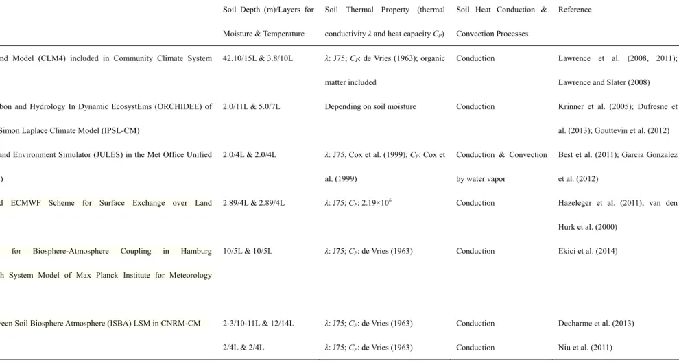
Table 1. The list of soil thermodynamics parameterizations in different LSMs/GCMs
Model Soil Depth (m)/Layers for
Moisture & Temperature
Soil Thermal Property (thermal conductivity λ and heat capacity CP)
Soil Heat Conduction & Convection Processes
Reference
Community Land Model (CLM4) included in Community Climate System Model-CCSM3
42.10/15L & 3.8/10L λ: J75; CP: de Vries (1963); organic
matter included
Conduction Lawrence et al. (2008, 2011);
Lawrence and Slater (2008) Organizing Carbon and Hydrology In Dynamic EcosystEms (ORCHIDEE) of
Institute Pierre Simon Laplace Climate Model (IPSL-CM)
2.0/11L & 5.0/7L Depending on soil moisture Conduction Krinner et al. (2005); Dufresne et al. (2013); Gouttevin et al. (2012) the Joint UK Land Environment Simulator (JULES) in the Met Office Unified
Model (MetUM)
2.0/4L & 2.0/4L λ: J75, Cox et al. (1999); CP: Cox et
al. (1999)
Conduction & Convection by water vapor
Best et al. (2011); Garcia Gonzalez et al. (2012)
Hydrology-Tiled ECMWF Scheme for Surface Exchange over Land (H-TESSEL)
2.89/4L & 2.89/4L λ: J75; CP: 2.19×10⁶ Conduction Hazeleger et al. (2011); van den
Hurk et al. (2000) Jena Scheme for Biosphere-Atmosphere Coupling in Hamburg
(JSBACH)-Earth System Model of Max Planck Institute for Meteorology (MPI-ESM)
Interaction between Soil Biosphere Atmosphere (ISBA) LSM in CNRM-CM Noah LSM 10/5L & 10/5L 2-3/10-11L & 12/14L 2/4L & 2/4L λ: J75; CP: de Vries (1963) λ: J75; CP: de Vries (1963) λ: J75; CP: de Vries (1963) Conduction Conduction Conduction Ekici et al. (2014) Decharme et al. (2013) Niu et al. (2011)
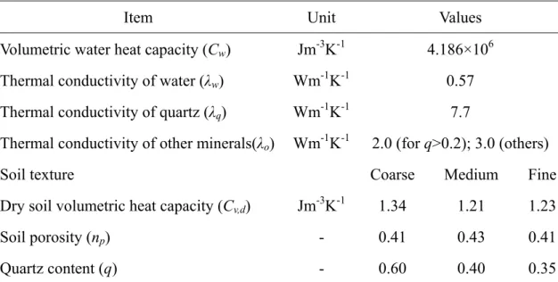
Table 2. The soil thermal property parameters
Item Unit Values
Volumetric water heat capacity (Cw)
Thermal conductivity of water (λw)
Thermal conductivity of quartz (λq)
Thermal conductivity of other minerals(λo)
Jm-3K-1 Wm-1K-1 Wm-1K-1 Wm-1K-1 4.186×10⁶ 0.57 7.7 2.0 (for q>0.2); 3.0 (others)
Soil texture Coarse Medium Fine
Dry soil volumetric heat capacity (Cv,d) Jm-3K-1 1.34 1.21 1.23
Soil porosity (np) - 0.41 0.43 0.41
Quartz content (q) - 0.60 0.40 0.35
The λw, λq, λo, np and q are obtained from Peters-Lidard et al. (1998). The Cv,d is
obtained from Pielke (2002). The coarse, medium and fine soil textures correspond to the sandy loam, loam and clay loam USDA textures classes, respectively.
28
Table 3. The soil vertical discretizations of 5M7L, 2M11L and 8M17L
5M7L 2M11L 8M17L
layer zz (m) zl (m) zz (m) zl (m) zz (m) zl (m)
1 1.419E-2 3.426E-2 0 0.978E-3 0/0.489E-3* 0.978E-3
2 6.264E-2 1.028E-1 1.955E-3 3.910E-3 1.955E-3 3.910E-3 3 1.595E-1 2.398E-1 5.865E-3 9.775E-3 5.865E-3 9.775E-3 4 3.533E-1 5.139E-1 1.369E-2 2.151E-2 1.369E-2 2.151E-2
5 7.409E-1 1.062 2.933E-2 4.497E-2 2.933E-2 4.497E-2
6 1.516 2.158 6.061E-2 9.189E-2 6.061E-2 9.189E-2 7 3.066 4.351 1.232E-1 1.857E-1 1.232E-1 1.857E-1
8 2.483E-1 3.734E-1 2.483E-1 3.734E-1
9 4.985E-1 7.488E-1 4.985E-1 7.488E-1
10 9.990E-1 1.500 9.990E-1 1.500 11 2.000 2.000 2.000 2.500 12 3.001 3.501 13 4.002 4.502 14 15 16 17 5.003 6.004 7.005 8.006/7.755* 5.503 6.504 7.505 8.006
zz: the depth at discretized node; zl: the depth at layer interface; *: 0 m and 8.006 m
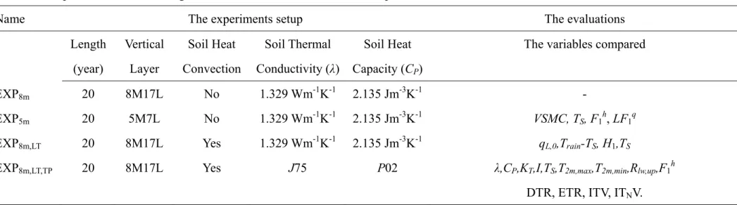
Table 4. The parameterization settings and evaluations for LMDZOR 3-D experiments
Name The experiments setup The evaluations
Length (year) Vertical Layer Soil Heat Convection Soil Thermal Conductivity (λ) Soil Heat Capacity (CP)
The variables compared
EXP8m EXP5m EXP8m,LT EXP8m,LT,TP 20 20 20 20 8M17L 5M7L 8M17L 8M17L No No Yes Yes 1.329 Wm-1K-1 1.329 Wm-1K-1 1.329 Wm-1K-1 J75 2.135 Jm-3K-1 2.135 Jm-3K-1 2.135 Jm-3K-1 P02 - VSMC, TS, F1h, LF1q qL,0,Train-TS, H1,TS
λ,CP,KT,I,TS,T2m,max,T2m,min,Rlw,up,F1h
DTR, ETR, ITV, ITNV.
The wind speed is ‘nudged’ by 6-hour relaxing time for all simulations. The ‘8m’, ‘5m’, ‘LT’ and ‘TP’ mean 8 m discretization, 5 m discretization, soil heat convection by liquid water transfer and soil thermal property, respectively. The VSMC, TS, F1h, LF1q, qL,0, Train, H1, λ, CP,
KT, I, T2m,max, T2m,min, and Rlw,up mean volumetric soil moisture content, surface temperature, sensible heat flux, latent heat flux, water flux at
surface, rain temperature, rain heat flux, soil thermal conductivity, soil heat capacity, soil heat diffusivity, soil thermal inertia, daily maximum air temperature, daily minimum air temperature, and upward long-wave radiation. The DTR, ETR, ITV, and ITNV mean Diurnal Temperature
Range, intra-annual Extreme Temperature Range, inter-diurnal temperature variability of the daily mean (ITV) and of the minimum temperature
30
Figure 1. The variation of (a) soil thermal conductivity λ and (b) soil heat capacity CP
with volumetric soil moisture for different soil textures (coarse, medium, fine) by using ORCHIDEE standard parameterization and the revised parameterization (λ is revised by using J75 method, and CP is revised by using P02 data).
0 0.5 1 1.5 2 2.5 0.00 0.05 0.10 0.15 0.20 0.25 0.30 0.35 0.40 so il th erm a l co nduc ti vi ty (W m -1K -1)
volumetric soil moisture (m3m-3)
λ_ORC λ_J75_coarse λ_J75_medium λ_J75_fine (a) 1 1.5 2 2.5 3 3.5 0.00 0.05 0.10 0.15 0.20 0.25 0.30 0.35 0.40 so il vol um . he a t ca p a .( M J m -3K -1)
volumetric soil moisture (m3m-3)
Cp_ORC Cp_P02_coarse Cp_P02_medium Cp_P02_fine
Δzk Δz11 Δzk+1 λk,Gk-1 Tk, θk, usk, CP,k λk+1,Gk λ17,G16 us17,CP,17 T17,θ17 qL,k+1 qL,17 qL,0 qL,k qL,k-1
Rad. & turbulent flux; εδT4
Δzk+1 Δzk Δzk-1
Δz17
Rad. & turbulent flux; εδT4
Δzk Δzk+1 Δzk-1
Δz7
(a) 5M7L for soil temperature (c) Revised 8M17L for moisture and temperature
(b) 2M11L for soil moisture
Figure 2. The soil vertical discretization of (a) 5M7L (Hourdin, 1992), (b) 2M11L (de Rosnay et al., 2000), and (c) 8M17L (new). The dashed and solid lines are the node and interface, respectively. For 2M11L, the top layer/bottom layer node and interface are at the same position. The heat transferred by liquid water at the bottom layer (qL,17)
is zero. θ, volumetric soil moisture (m3m-3); qL, liquid water flux (ms-1),
qLi=-0.5×(D(θi-1)+D(θi))×(θi-θi-1)/Δzi+0.5×(K(θi-1)+K(θi)); D, hydraulic diffusivity
(m2s-1); K, hydraulic conductivity (ms-1); us, water uptake due to transpiration (no transpiration at the top layer); T, soil temperature (K); G: soil heat flux (Wm-2); zz, zl: soil depth at node and interface, respectively (m); Δz, thickness of each layer (m); CP,
32
Figure 3. The variation of required soil depth for simulating annual cycles of soil temperature/heat flux with volumetric soil moisture (a), and the variation of soil temperature/heat flux amplitude decaying ratio with soil layers (b) for different soil textures: Coarse (COA), Medium (MED) and Fine (FIN). The soil heat convection by liquid water transport (8.64 mm d-1) is considered in ‘L’, and it is excluded in ‘NL’.
3.0 4.0 5.0 6.0 7.0 8.0 0 0.05 0.1 0.15 0.2 0.25 0.3 0.35 0.4 S o il D ept h( m )
Volumetric Soil Moisture (m3m-3)
DD_COA(NL) DD_COA(L) DD_MED(NL) DD_MED(L) DD_FIN(NL) DD_FIN(L) (a) 0 0.1 0.2 0.3 0.4 0.5 0.6 0.7 0.8 0.9 1 1 2 3 4 5 6 7 8 9 10 11 12 13 14 15 16 17 A m p litu d e D eca y in g R a tio Soil Layer AMP_COA(NL) AMP_COA(L) AMP_MED(NL) AMP_MED(L) AMP_FIN(NL) AMP_FIN(L) e^(-3) (b)
Figure 4. The comparison of daily soil temperature (T, a and b) and soil heat flux (G, c and d) between analytical method (AM) and finite difference method (FDM) for soil heat conduction-convection model by using 8M17L discretization with liquid water flux qL = 1E-7 ms-1 (8.6 mm d-1): time serials (a, c) and vertical profiles (b, d).
290 291 292 293 294 295 296 297 298 0 30 60 90 120 150 180 210 240 270 300 330 360 T em p era tu re( K ) Day T_AM_1L T_FDM_1L T_AM_17L T_FDM_17L (a) 290 292 294 296 298 300 0 1 2 3 4 5 6 7 8 9 10 11 12 13 14 15 16 17 T em p era tu re (K ) Soil Layer AM_90D FDM_90D AM_270D FDM_270D AM_180D FDM_180D AM_360D FDM_360D (b) -2.5-2 -1.5-1 -0.5 0 0.51 1.52 2.5 0 30 60 90 120 150 180 210 240 270 300 330 360 S o il H ea t F lu x (W m -2) Day G_AM_0L G_FDM_0L G_FDM_16L G_AM_16L (c) -2 -1.5 -1 -0.5 0 0.5 1 1.5 2 0 1 2 3 4 5 6 7 8 9 10 11 12 13 14 15 16 S o il H ea t F lu x (W m -2) Soil Layer AM_90D FDM_90D AM_270D FDM_270D AM_180D FDM_180D AM_360D FDM_360D (d)
34
Figure 5. The results of EXP8m (8M17L, left) and the difference between EXP5m
(5M7L, Table 4) and EXP8m (right): (a, b) volumetric soil moisture content at 0-1.5 m;
(c, d) surface temperature TS; (e, f) sensible heat flux F1h and (g, h) latent heat flux
Figure 6. The vertical profiles of soil temperature in MAM (a), JJA (b), SON (c) and DJF (d) over South Africa (50W-70W, 5S-20S) for 8M17L (EXP8m) and 5M7L
36
Figure 7. (a) liquid water flux at surface; (b) difference between rain and surface temperature; (c) heat fluxes by convection at surface for EXP8m,LT (Table 4), and (d)
differences in surface temperature due to the heat transferred by rain and water into the soil (differences between EXP8m,LT and EXP8m). All values are annual mean.
Figure 8. The LMDZOR simulations (annual mean) for EXP8m (left) and the
differences between EXP8m,LT,TP (Table 4) and EXP8m (right) for (a) soil thermal
conductivity; (b) soil heat capacity; (c) soil thermal inertia; (d) soil heat diffusivity; (e, f) surface temperature; (g, h) daily maximum temperature; (i, j) daily minimum temperature; (k, l) upward long-wave radiation; and (m, n) sensible heat flux. The white regions indicate that the new parameterizations are not significant.
38
Figure 9. The extreme climate variables for EXP8m (left) and its difference with
Figure 10. The probability density function (PDF) for DTR (1st column) and ITNV
(2nd column), and the box plot of DTR (3rd column) and ITNV (4th column) over the
Sahara (1st line), the Sahel (2nd line), the central US (3rd line) and north China (4th line) between EXP8m,LT,TP and EXP8m with daily values. The grid point value is
weighted by its areas. In the box plot, the red central mark and the blue dot are the median and mean, and the edges of the box and the 25th and 75th percentiles. The whiskers extend to the most extreme data points not considered outliers. Points are drawn as outliers if they are larger than X25th + 3*(X75th - X25th) or smaller than X25th –
3*(X75th - X25th), where X25th and X75th are the 25th and 75th percentiles respectively.
The red diamond and the values are the 99th and 1st percentiles. The percentage (%, dSTD, dSkewness in PDF; values in brackets in box plot) measures the difference between the two simulations: (EXP8m,LT,TP - EXP8m)/ EXP8m*100%.