HAL Id: hal-00298041
https://hal.archives-ouvertes.fr/hal-00298041
Submitted on 8 Dec 2005
HAL is a multi-disciplinary open access
archive for the deposit and dissemination of
sci-entific research documents, whether they are
pub-lished or not. The documents may come from
teaching and research institutions in France or
abroad, or from public or private research centers.
L’archive ouverte pluridisciplinaire HAL, est
destinée au dépôt et à la diffusion de documents
scientifiques de niveau recherche, publiés ou non,
émanant des établissements d’enseignement et de
recherche français ou étrangers, des laboratoires
publics ou privés.
Seasonal mean pressure reconstruction for the North Atlantic
(1750–1850) based on early marine data
D. Gallego1, R. Garcia-Herrera2, P. Ribera1, and P. D. Jones3
1Departamento de Ciencias Ambientales, Universidad Pablo de Olavide, Sevilla, Spain 2Departamento de Fisica de la Tierra II, Universidad Complutense, Madrid, Spain 3Climatic Research Unit, University of East Anglia, Norwich, UK
Received: 14 June 2005 – Published in Climate of the Past Discussions: 8 August 2005 Revised: 19 October 2005 – Accepted: 22 November 2005 – Published: 8 December 2005
Abstract. Measurements of wind strength and direction ab-stracted from European ships’ logbooks during the recently finished CLIWOC project have been used to produce the first gridded Sea Level Pressure (SLP) reconstruction for the 1750–1850 period over the North Atlantic based solely on marine data. The reconstruction is based on a spatial re-gression analysis calibrated by using data taken from the ICOADS database. An objective methodology has been de-veloped to select the optimal calibration period and spatial domain of the reconstruction by testing several thousands of possible models. The finally selected area, limited by the per-formance of the regression equations and by the availability of data, covers the region between 28◦N and 52◦N close to the European coast and between 28◦N and 44◦N in the open
Ocean. The results provide a direct measure of the strength and extension of the Azores High during the 101 years of the study period. The comparison with the recent land-based SLP reconstruction by Luterbacher et al. (2002) indicates the presence of a common signal. The interannual variability of the CLIWOC reconstructions is rather high due to the cur-rent scarcity of abstracted wind data in the areas with best response in the regression. Guidelines are proposed to opti-mize the efficiency of future abstraction work.
1 Introduction
The study of long climatological series at scales longer than the period covered by traditional instrumental data is es-sential to study both the natural variability and any anthro-pogenic effect in the climatic system. In particular, the knowledge of the Sea Level Pressure (SLP) over large ex-tensions provides a direct measure of the atmospheric circu-lation and offers a more consistent analysis of climate
vari-Correspondence to: D. Gallego
ability than the reconstruction of circulation indices based on a few key locations (Luterbacher et al., 2002). However, datasets including sea level pressure are only available since the mid 19th century. Currently, the most complete SLP grid-ded dataset (HADSLP2) has been recently developed at the Hadley Centre. This update of the well-known GMSLP2 dataset (Basnett and Parker, 1997) extends back to 1850.
The importance of estimating the SLP as early as possible is the origin of the numerous attempts to develop SLP charts based either on direct measures or through its effects on in-direct variables such as temperature or precipitation. The vast majority of the SLP reconstructions cover the Eurasian sector due to the higher availability of long climatic series in Europe. For example, Lamb and Johnson (1966) devel-oped one of the first reconstructions back to 1750, producing SLP charts for January and July. However, the subjective methodology used (hand-drawn charts) was focused on ob-taining “seasonal” SLP patterns rather than average monthly values. The development of computer-assisted methodolo-gies has increased the use of objective statistical techniques applied to climate reconstruction, mostly variants of multi-ple regression. These methodologies were applied by Jones et al. (1987), who developed monthly mean SLP reconstruc-tions back to 1780 and 1858 for Europe and North America respectively. Cook et al. (1994) critically compared two mul-tiple regression schemes and reconstructed the SLP back to 1750 by using tree-ring data from western Europe and east-ern North America. The finding of more monthly station pressure data allowed Jones et al. (1999) to improve the re-construction of the monthly mean SLP for Europe for the 1780–1995 period. Luterbacher et al. (2000), by including documentary and natural proxy data in addition to early in-strumental meteorological measures, reconstructed the SLP for the Late Maunder Minimum period (1675–1715) reach-ing monthly resolution. Recently, Luterbacher at al. (2002) pushed back the initial year of the monthly SLP reconstruc-tions to 1659 (1500 for seasonal data) in western Europe by
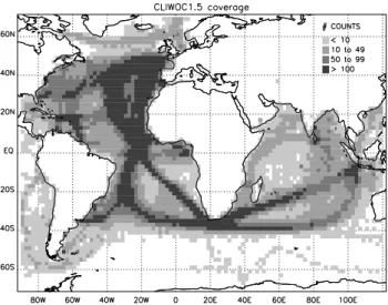
Fig. 1. Raw coverage of the CLIWOC 1.5 data for the period 1750–
1850 on a 2◦×2◦grid.
using a combination of early station series of pressure, tem-perature, precipitation and documentary data. A common characteristic of all these SLP reconstructions is their depen-dence on land-based observation series (predictors) used to develop the statistical relationship with the SLP (the predic-tand). With the exception of a few stations located on the European Atlantic islands (Azores and Madeira in the sub-tropical North Atlantic or Iceland in the northern North At-lantic) all the predictors are located in continental Eurasia. As a consequence, these gridded SLP reconstructions are not available westward of 30◦W and do not explicitly include oceanic data. Therefore, the available early gridded SLP over the eastern edge of the Atlantic are mostly based on the in-direct statistical connection among the oceanic pressure pat-terns with climate anomalies over continental Europe. The inclusion of marine data seems essential to improve current SLP reconstructions.
Before the establishment of the present observation net-works, meteorological measurements over the oceans were limited to those obtained aboard sailing ships. The In-ternational Comprehensive Ocean-Atmosphere Data Set (ICOADS, Woodruff et al., 1987) constitutes the world’s ex-tensive archive of marine data. Currently, version 2.1 of the database contains monthly summaries of SLP over the oceans back to 1800, although the data coverage before 1850 is extremely sparse (Woodruff et al., 2005). In this regard, the methodologies developed by Kaplan et al. during the last decade (1997, 2003) have produced optimal and nearly global SLP grids based on ICOADS back to 1854 (Kaplan et al., 2000), before that date there are simply too few data.
Between the years 2001 and 2003, the European Union funded CLIWOC project (Garcia-Herrera et al., 2005a) digi-tised early wind measurements taken aboard ships covering routes from Europe to America, Asia and Africa between
were homogenised and converted to standard units (m×s−1)
making possible their implementation in quantitative recon-struction algorithms. The particular details of the original data and the conversion can be consulted in Garcia-Herrera et al. (2005b), Koek and K¨onnen (2005); Prieto et al. (2005) and Wheeler and Wilkinson (2005).
The first attempt to find climatological signals in the CLI-WOC database was recently carried out by Jones and Salmon (2005), who reconstructed the North Atlantic Oscillation (NAO) and the Southern Oscillation with promising results. The aim of this paper is to explore the capability of the CLI-WOC database to provide a reconstruction of SLP over a large part of an oceanic basin. The paper is organised as follows. Section 2 describes the databases used. Section 3 summarises the reconstruction methodology, with emphasis on the importance of the selection of the study domain. Sec-tion 4 evaluates the performance of the model, while Sect. 5 provides some examples of the results comparing them with a previous reconstruction. Section 6 discusses some aspects of the results.
2 Data
2.1 CLIWOC data
For this study, the last available version of the CLIWOC database was used (version 1.5). The complete CLIWOC 1.5 database has 280 280 entries. From these, the 245 195 non-coastal data were included in this study. After a pre-liminary analysis, a total of 190 451 entries were found con-taining complete information about wind speed and direction for the 1750–1850 period. Figure 1 shows the data cover-age in open seas over a 2◦×2◦ grid. As expected, the best
densities are found over the most frequent routes, mainly over the Atlantic from western Europe to the Caribbean and South America and through the Atlantic and the South In-dian Ocean to Indonesia. Over the Pacific Ocean (not shown in Fig. 1) only a small number of data corresponding to iso-lated trips were found, because no regular routes existed dur-ing this period in this region. By far, the best coverage cor-responds to the eastern half of the North Atlantic because
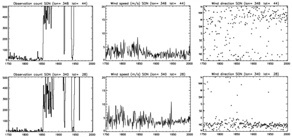
Fig. 2. Examples of numbers of counts, wind speeds and directions for two the 8◦×8◦squares centered at 44◦N–12◦W (upper panels) and 28◦N–20◦W (lower panels) based on CLIWOC data (up to 1850) and on ICOADS data (from 1851). The season shown is SON.
this area was a mandatory route for the Spaniards from Spain to the Caribbean and Argentina, the British from the United Kingdom mainly to North America and Asia and the Dutch from The Netherlands to South Africa and Indonesia. Ini-tially, the entire North Atlantic was considered in the recon-struction models but preliminary studies resulted in poor per-formances south of the Northern Hemisphere tropical area. In consequence the study region was limited to the North At-lantic as the regions with better data density.
2.2 ICOADS data
The vast majority of the CLIWOC data over the North At-lantic do not contain SLP measures to calibrate the rela-tion wind-SLP. Therefore, following the approach of Jones and Salmon (2005), in order to develop the regression equa-tions, the standard monthly summaries of ICOADS 2.1 has been used (Worley et al., 2005). This database contains the monthly u and v wind components, and the SLP from 1800 to 2002. However, for our purposes of evaluating the perfor-mance of the CLIWOC data, we did not use any ICOADS data for the pre-1851 period. The ICOADS database also contains monthly means of scalar wind, whose ratio with the magnitude of the vector wind can provide an indication of wind steadiness, however we did not use it for this study be-cause we were interested in the wind vector and its relation with SLP. It must be pointed out that despite the early begin-ning of the ICOADS database, the SLP data are very sparse before 1850 and there are virtually no SLP measures before 1830, even expanding the spatial resolution to an 8◦×8◦grid. 2.3 Data pre-processing
As a first step, to avoid obtaining regression equations that would reproduce mostly the seasonal cycle instead of the
in-terannual variability, both CLIWOC and ICOADS data were reduced to monthly anomalies using the period 1961–1990 as a base. That is, for each 2◦ square, the corresponding monthly 1961–1990 average was subtracted. As shown by Jones and Salmon (2005), a 2◦×2◦grid on a monthly basis for the current CLIWOC coverage does not provide enough data density to perform useful climatic reconstruction. The CLIWOC and ICOADS monthly anomalies were aggregated up to an 8◦×8◦ resolution. Instead of the original monthly
series, seasonal averages were computed for the boreal win-ter (DJF), spring (MAM), summer (JJA) and autumn (SON). Even with this approach the number of CLIWOC counts is appreciably lower than that corresponding to the post 1851 ICOADS period. However the wind vectors show consistent values when compared with the modern data. Figure 2 shows two examples of the raw 8◦x8◦ data for two regions over the eastern North Atlantic for areas representing the west-erlies (8◦×8◦square centered at 44◦N–12◦W) and the sub-tropical region (8◦×8◦square centered at 28◦N–20◦W). The scarce number of data prior to 1851 is evident in both cases, showing some missing values (years with no CLIWOC data) around 1810. However, despite the lower amount of data (though comparable to the World Wars I and II periods, see Fig. 2), the average wind strength and direction for the CLI-WOC period shows fairly consistent values, similar to the ICOADS averages from 1851 onwards. The magnitude of the average wind vector at 44◦N oscillates around 3 to 4 m/s with slightly greater and more variable values during 1800– 1850, clearly related with a decrease in the amount of data. For this gridpoint, the direction shows a dominance of the N-NW component with a high interannual variability both for ICOADS and CLIWOC datasets. In the subtropical exam-ple, the lower variability associated with the trade wind belt is evidenced in more stable averages. Around 28◦N, close
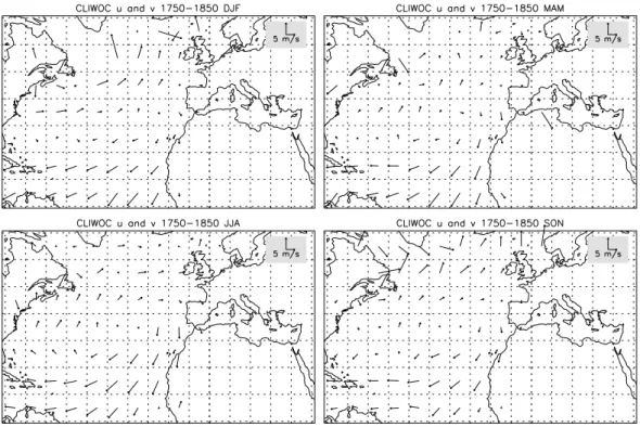
Fig. 3. Initial set of 8◦×8◦squares over the North Atlantic included in the study. In the center of each square the average CLIWOC wind vectors for the entire 1750–1850 period are shown.
to the Canaries, the wind speed fluctuates around 4 m/s with a clear NE component. For both cases, the lower amount of data in the CLIWOC case is manifested as an increase in the interannual variability rather than in changes of the average values.
Figure 3 shows the complete set of 8◦×8◦ CLIWOC squares over the North Atlantic initially included as potential predictors in this study. The typical structure of the winds around the Azores high is evident and some erratic vectors on the northern edge of the area can be seen, linked to a very low number of observations.
3 Methodology
3.1 Reconstruction method
The reconstruction of SLP over the oceanic North Atlantic as a function of the u and v wind components has been car-ried out by applying the orthogonal spatial regression (OSR) technique. The OSR has been widely used during the last decades to reconstruct climatic series (Jones et al., 1987; Briffa et al., 1992; Cook et al., 1994; Jones et al., 1999; Jones and Salmon, 2005 among others) and has proven adequate to reconstruct climatic fields based on variables with strong interdependences as will be the case of the u and v compo-nents of the wind. Here only a brief introduction is provided. The complete mathematical details of the OSR can be seen in Jones et al. (1987).
The most usual problem of the regression techniques ap-plied to climatic reconstruction consist in the tendency to overfit the data offered for regression. Climatic series over a region, especially those coming from non-instrumental sources, usually show strong interdependences and contain a lot of potentially redundant information. The OSR per-forms regression not over the raw set of predictors (u and v over a grid in our case) against a set of predictands (SLP) but over the amplitude time series of a subset of their principal components (PCs) with the aim of excluding from the model most of the spurious information. Once the regression equa-tions for a calibration period are established, the stability of the relationship is assessed by applying the model to a ver-ification period independent of the calibration one. Finally, the equations can be applied to the reconstruction and the resulting PCs are transformed back to the original variables.
3.2 Selection of the regression model
Usually the number of predictors and predictands to be in-cluded in a regression model is imposed by the availability of data during the reconstruction period. The problem of time-varying predictor networks is usually solved by adjust-ing different regression equations as the number of available predictors increases (Jones et al., 1987; Jones et al., 1999). In the CLIWOC case, the low number of data north of 50◦N and westward of 50◦W is evident from Fig. 1. In fact, no se-ries are complete, even for the 8◦×8◦seasonal dataset. How-ever, there is not a simple increase in the number of available
56W 48W 40W 32W 24W 16W 8W 56W 48W 40W 32W 24W 16W 8W 56W 48W 40W 32W 24W 16W 8W 56W 48W 40W 32W 24W 16W 8W 24N 32N 40N 48N 24N 32N 40N 48N 56N
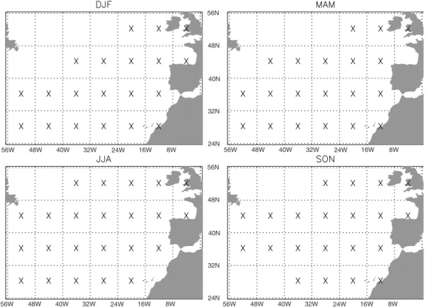
Fig. 4. Final 8◦×8◦squares used in the reconstruction model.
predictors between 1750 and 1850 but a random-like distri-bution of missing values during the entire period (both in space and time). To make a better use of the information contained in the predictor network, the missing seasonal val-ues for the anomalies were assumed to be zero (Jones and Salmon, 2005). This procedure inevitably adds uncertainty to the reconstruction, but, on the other hand, allows the inclu-sion of a great amount of valuable information which would be discarded otherwise. Initially, all the gridpoints included in Fig. 3 were considered as candidate predictands and, in or-der to search for the optimal set, a methodical approach was designed by testing different regression models varying the following parameters:
– Calibration and verification periods. The following calibration periods were tested: 1881–1940 (same as in Jones and Salmon 2005), 1931–1960 (a 30-year standard climate period), and 1851–1925 (approxi-mately the first half of the complete period of available ICOADS data). For verification, 1941–2000 (same as in Jones and Salmon, 2005), 1961–1990 (the standard 30-year climatic period following the corresponding period used in calibration) and 1926–2000 (second half of the complete period of ICOADS data) were tested. As an additional test, we interchanged the order of the veri-fication and calibration periods for the first case, i.e. a model with calibration period 1941–2000 and verifica-tion period 1881–1940.
– Level of variance retained prior to regression. The selection of the PCs retained was undertaken by pre-selecting a desired level of explained variance (Fritts et al., 1971). The levels 70%, 80%, 90% and 95% were independently tested for predictors and predictands.
– Number and location of the gridpoints included in the model. Every sub-region between the squares centred at 76◦W and 4◦W and between 12◦N and 60◦N (Fig. 3) was tested.
A total of 6928 different models were tested. In each case, during the regression, the retained PCs with a t -value lower than 1 were excluded from the equations (Briffa et al., 1983; Jones et al., 1987). The average temporal correlation for all the included gridpoints between real and reconstructed series for the calibration and verification period was used as the criterion to select the optimal regression equations.
The model with best correlation was the one calibrated for 1931–1960 with verification period 1961–1990. Both for predictors and predictands, we retained the first n PCs such that at least 95% of the total variance was retained. The final 8◦×8◦squares included in the reconstruction cover the area from 28◦N to 52◦N and from 52◦W to 4◦W, although not all the squares inside that region could be included because of absence of data. Figure 4 shows the included squares for each season. No SLP reconstruction was developed for squares different to those shown in Fig. 4. Previous reconstructions
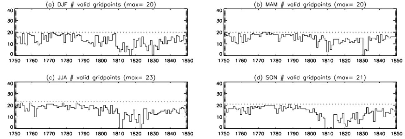
Fig. 5. Number of 8×8 squares for wind included (not missing) in the SLP reconstruction as a function of the time. Dotted horizontal line
indicates the maximum possible number for the selected area.
(see Luterbacher et al., 2002 for example) based on the re-lationship between SLP and precipitation and temperature data take advantage of the long-range influence of the cir-culation on these variables and in consequence perform the reconstruction over areas wider that those covered by the pre-dictors. In our case, the close relationship between SLP and wind measurements indicates a reconstruction for the same grid covered by the predictors.
Even with the careful selection carried out, there are still missing data in the predictor series. Figure 5 shows the an-nual number of extant gridded wind data used in the recon-struction as a function of the time. The maximum possible number of predictors (number of crosses in Fig. 4) is also shown. In general, during the first half of the reconstruction period there is a better coverage. A shortage of data is ev-idenced between 1810 and 1830, with a slow improvement until 1850. During the cold half of the year, the number of observations is lower, due to the preference of the captains to cross the Atlantic during the usually less stormy warm season. This fact is particularly evident for the DJF period 1810–1820 (Fig. 5a) and SON around 1810 (Fig. 5d).
3.3 Verification tests
The reliability of the regression equations was assessed by using an approach similar to that employed in dendroclima-tological analysis. Six different indices were computed. A complete description of the different tests and their signifi-cance is provided by Cook et al. (1994):
– Temporal correlation coefficient between the ICOADS SLP series and the reconstruction for the calibration and verification periods at each gridpoint.
– Spatial correlation of SLP for the entire 1850–2002 pe-riod. The temporal mean from each point was sub-tracted before this analysis in order to avoid represent-ing mostly the seasonal cycle.
Table 1. Number of original squares included in each seasonal
model (Raw), number of retained PCs (Ret. PCs) and % of variance explained by the retained PCs (% Var.).
Predictor (u, v) Predictands (SLP) Raw Ret. PCs % Var. Raw Ret. PCs % Var. DJF 40 14 95.2 20 8 95.6 MAM 40 14 95.3 20 9 96.1 JJA 46 15 95.6 23 10 95.5 SON 42 12 95.7 21 9 95.4
– Sign test: The similarity between series is evaluated by counting the number of agreements in sign between real and reconstructed anomaly series.
– Product means test: This compares the magnitude of the mean positive and negative cross products of the actual and reconstructed departures from the mean SLP.
– Reduction of Error (Lorenz, 1956): This compares the reconstructed series with the climatology during the cal-ibration period. This statistic ranges from minus infini-tum to +1.0. Values greater than zero indicate that the reconstruction is better than climatology during the cal-ibration period.
– Coefficient of Efficiency (Briffa et al., 1988): Formally identical to the reduction of error, it compares the re-construction with the climatology during the verifica-tion period. A coefficient of efficiency greater than zero indicates useful information in the climate reconstruc-tion.
4 Model adjustment and performance
Table 1 shows the number of PCs necessary to retain at least 95% of the variance. Approximately a third of the PCs for
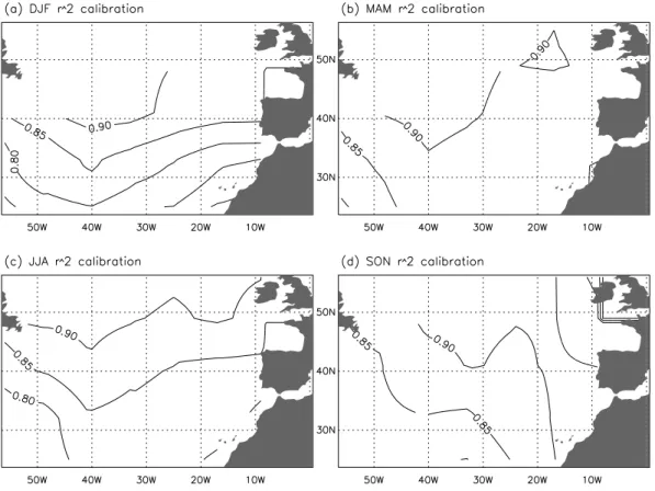
Fig. 6. Seasonal model performance (R2)for the calibration period (1931–1960).
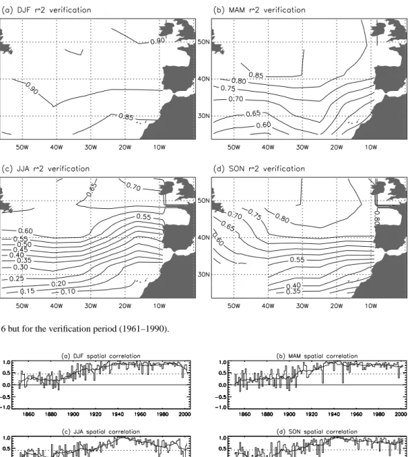
predictors and a half of the predictands were retained, with no evident seasonal changes. The model performance for the calibration period is displayed in Fig. 6. All the seasons show similar features. In general the best R2are found for the northern squares reaching 0.90 to 0.95. R2 values de-crease smoothly toward the south, with values between 0.80 and 0.85 in the subtropical North Atlantic. The results for the verification period are displayed in Fig. 7. The stability of the regression equations during winter is evident (Fig. 7a).
R2values during this season are well above 0.80 for all the included squares, again with better values toward the north. Spring and autumn show a good response as well over the northern half of the domain. However a fast decrease of R2 to the south is evident for these seasons, especially during the autumn, with values around 0.40 below 30◦N. Finally, the poorest response of the model is observed for the summer. Only northward of 50◦N, R2values are above 0.60 (Fig. 7c). During this season, the decrease in the performance to the south is fast, and in the subtropical latitudes R2is typically 0.30.
The spatial correlation analysis is shown in Fig. 8. The best performance, as expected, is found for the calibration period. In general, from 1930 on, apart from the summer season, the spatial correlation shows a remarkably good re-sponse, before 1930, the spatial performance is poorer. Evi-dently, the number of observations plays an important role in SLP reconstruction. A greater amount of data results in
bet-Table 2. Some statistics summarising the model performance. rc
and rvindicates the average correlation for the calibration and
ver-ification periods over the study area. Numbers in brackets indicate the number of significant correlations versus the total number of squares. The columns ST and PT indicate the number of squares passing the sign test and the product means test respectively versus the total number of squares (significance levels set to 95%). RE and CE indicate the averaged reduction of error and coefficient of efficiency (see text for details).
rc rv ST PM RE CE
DJF 0.914 (20/20) 0.943 (20/20) 20/20 20/20 0.855 0.853 MAM 0.939 (20/20) 0.851 (20/20) 19/20 20/20 0.635 0.511 JJA 0.930 (20/23) 0.614 (15/23) 14/23 13/23 0.240 0.100 SON 0.936 (20/21) 0.785 (19/21) 18/21 18/21 0.499 0.419
ter reconstructions. Nevertheless, the coarse 8◦×8◦grid used implies that the reconstruction area is covered by a relatively small number of points and relatively small differences in reconstructed and observed SLP at the edges of the domain (usually the points with poorer coverage) can have a large effect on the spatial correlations.
As a summary, Table 2 shows the principal quality con-trol statistics for the calibration and verification periods. The values show that the model performs remarkably well with the exception of the summer season, with the vast majority
Fig. 7. As Fig. 6 but for the verification period (1961–1990).
Fig. 8. Spatial correlation for the 1851–2002 period. Smoothed line corresponds to the 11-year running average. Significance level (p<0.05)
is indicated by the dashed line.
of the squares included in the model passing the entire set of tests. The model performance strongly depends on the number and especially the location of the squares included in the reconstruction area. A fast decrease in performance was observed for those models including squares southward of 28◦N, even though the CLIWOC data quality is similar to that of the northern squares. In this regard, there are two rea-sons for the observed model degradation toward the South. First, the different relationship between SLP and wind in the equatorial zone relative to that observed at mid latitudes
pre-vented adjusting the wind data with similar equations. Sec-ond, the SLP anomalies are much smaller in the tropics and subtropics than over midlatitude areas and, in consequence, the relative errors both in the input data and in the recon-struction are higher. In addition, the model adjustment may be affected by the reduced ICOADS coverage for the eastern side of the subtropical North Atlantic compared with that of northern areas. Mid-latitude squares westward of 56◦W and
north of 60◦N performed well in the regression but they were
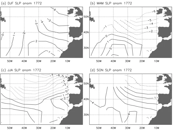
Fig. 9. Reconstructed seasonal SLP anomaly (hPa) relative to the 1961–1990 ICOADS average for 1772. Contours plotted every 1 hPa.
Negative SLP anomalies are indicated by dotted contours.
5 Results
Two examples of reconstructed SLP anomalies relative to the 1961–1990 period are displayed in Figs. 9 and 10. Figure 9 shows an example for 1772 a year with a high number of available predictors (see Fig. 5). The reconstruction shows positive SLP anomalies for the subtropical Atlantic during the year and lower than present-day averages during spring and summer (Figs. 9b and 9c for latitudes over 30◦N). The large SLP anomalies range from −6 to 6 hPa and are prob-ably excessive considering the seasonal nature of the recon-struction. The likely cause of these large values is the rela-tively low number of wind measurements causing larger than expected variability in the wind anomalies, even during the most favorable dates and areas (first half of the 18th century and the North Atlantic Ocean, see Fig. 2). This subject will be discussed further in the next section.
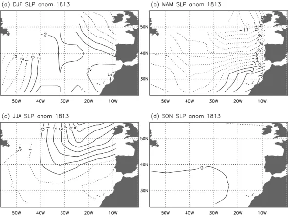
Figure 10 shows an example for 1813, a year of reduced CLIWOC coverage over the North Atlantic. For this year, only about 50% of the squares are available during winter, spring and summer (Figs. 5a to 5c) and there are no data at all for autumn (Fig. 5d). The effects of the poorer coverage on the reconstruction are evident. During winter (Fig. 10a), the anomaly SLP field shows the central Azores high only slightly stronger than the 1961–1990 average. During this
season, the SLP anomalies are no larger than 3 hPa. On the contrary, during spring (Fig. 10b), large negative anomalies reaching −11 hPa can be seen around 45◦N. For the sum-mer (Fig. 10c) strong positive anomalies up to 6 hPa cover the northern reconstruction area. These results suggest that the effect of the reduced data coverage is more critical during the seasons with less organization of the atmospheric circu-lation. Figure 10d shows the case of reconstructions with no CLIWOC data (zero wind anomalies, according to the crite-ria followed for missing values) and the consequent repro-duction of the ICOADS 1961–1990 seasonal averages.
The complete temporal evolution of the SLP for winter is shown in Fig. 11 for decadal averages. In general, the recon-structed SLP shows a tendency to be above the 1961–1990 values over the southern boundary of the study area (squares centered at 28◦N) with the exception of a 20-year period starting around 1781. Northern latitudes over the central North Atlantic show larger variability, with anomalies close to zero during 1751–1770, negative between 1771 and 1800 and positive after 1801. With the exception of the decade starting in 1781, the reconstructed SLP shows positive val-ues along the western European coast, with larger anomalies close to the British Isles.
An example of the temporal evolution of the reconstructed SLP for the square centered at 36◦N/36◦W is shown in
Fig. 10. As Fig. 9 but for 1813.
Fig. 12. This particular point is close to the centre of the study domain and represents the strength of the Azores High. The principal characteristic of the reconstruction is the great variability exhibited during all the four seasons, especially during the first half of the study period. The in-terannual variability is greater during the cold half of the year with values ranging between 1030 hPa (1782 and 1785) and 1004 hPa (1784) for winter and between an exceptionally high 1039 hPa followed by 1030 hPa (1773 and 1796 respec-tively) and 1005 hPa (1769) for autumn. During the sum-mer the values range between 1034 hPa (1759) and 1012 hPa (1760). For spring these extremes are 1030 hPa (1755) and 1009 hPa (1785) respectively. As a comparison, the 1961– 1990 ICOADS average for the SLP over the corresponding square has been displayed in Fig. 12. Regarding the interan-nual variability, it is perceptibly lower during the second half of the study period.
The recent reconstruction of Luterbacher et al. (2002, L02 subsequently), based on land data covering the eastern North Atlantic and Europe is considered one of the best SLP re-constructions over the Atlantic at present and it provides a monthly SLP dataset back to 1659 on a 5◦×5◦ grid reach-ing 30◦W. In addition this reconstruction includes predictors well into the Atlantic using data for the Azores and Madeira (though only from 1865) and Iceland (from 1821), making the L02 data probably the best series to compare with the
CLIWOC reconstruction. As the grid is different and due to the coarse spatial resolution of both reconstructions, a direct point-to-point comparison is difficult because up to four dif-ferent L02 series can be included inside one 8◦×8◦CLIWOC square. Instead of computing correlation maps, five CLI-WOC squares representative of the study domain from the westward limit of the L02 data (30◦W) to the European coast (12◦W) and from the CLIWOC latitudes 36◦N, 44◦N and 52◦N (the 28◦N latitude is not included in L02) have been selected. The selected L02 5◦×5◦ gridpoint is that whose center is closer to its corresponding CLIWOC counterpart. Three statistics have been computed on a seasonal basis for the 1750–1850 period: the temporal correlation, the average SLP and the standard deviation.
Figure 13 shows that all the correlation coefficients but one are positive. However, significant seasonal differences can be clearly seen. The larger correlations are attained for win-ter, with statistically significant values for four out of the five points. Interestingly, the best correlated point (r=0.437) is located near the Iberian coastline: this is the square with best CLIWOC coverage and it is located over a location closer to the majority of the L02 data. Excluding winter, the corre-lations are still positive but noticeably lower. The statistical significance is reached two times for autumn and spring and once for summer. The average CLIWOC SLP is in all cases well below the corresponding L02 value by an average of
Fig. 11. Reconstructed decadal SLP anomaly (hPa) relative to the 1961–1990 ICOADS average. Contours plotted every 0.5 hPa. Negative
Fig. 12. Reconstructed SLP for the period 1750–1850 for the 8◦×8◦square centered at 36◦N–36◦W. Smooth line represents the 5-year moving average. Dashed horizontal line indicates the corresponding ICOADS average for 1961–1990.
3.4 hPa for the selected points but the main difference oc-curs in the magnitude of the interannual variability, which is 2.6 times larger on average for the CLIWOC data than for the L02 reconstruction. Despite the dissimilarities, the char-acter of the variability seems similar. When L02 has large anomalies, so does the CLIWOC reconstruction. This fact is evidenced in Fig. 13, which shows that large averaged devia-tions in L02 are corresponded by large values of its CLIWOC counterpart.
6 Summary and discussion
Orthogonal spatial regression has been applied to reconstruct the SLP over a large part of the North Atlantic based on early wind measurements taken aboard Spanish, British, French and Dutch ships for the period 1750–1850. This is the first SLP reconstruction over this region and period based uniquely on marine data.
Early reconstructions attempts showed that the definition of the study domain was very important. By far, the best coverage offered by CLIWOC is located in the North At-lantic, which was selected as the study area. The verifica-tion tests over a larger region of the Atlantic between 15◦N to 50◦N showed a fast degradation in performance south-ward of 30◦N and serious coverage problems westward of 50◦W. As a result of these initial experiments, a methodi-cal approach based on testing a batch of regression models with different explained variances, study areas and calibra-tion/verification periods was adopted. The selected domain, based on achieving the best correlation between the ICOADS and modeled SLP during the calibration and the verifica-tion periods, covers the region from 28◦N to 52◦N and be-tween 52◦W and 4◦W. The elimination of the grid points westward of 52◦W and northward of 52◦N results from the low number of CLIWOC observations while the selection of the southern boundary is imposed by the performance of the
model, as plenty of CLIWOC data were available over the subtropical North Atlantic.
Once an adequate region was selected, a reconstruction based on the OSR performed remarkably well in winter, with verification correlations almost as high as the calibra-tion ones. The quality of the reconstruccalibra-tion, as measured by the different test implemented strongly depends on the sea-son and region. The verification correlations decrease during transitional seasons and the worst response is obtained dur-ing the summer. The strong dependence of the model per-formance on the season stresses the necessity of working at least at seasonal scales. No attempt to use single monthly data was made due to the low number of observations. A reduction in verification and calibration correlations toward the south was found. This decrease is rather low for winter, a season with high values of R2even southward of 30◦N but it limits the usefulness of the reconstructions southward of 35– 40◦N during the rest of the year. This result should be a key point in future efforts to abstract logbook data. While the best responses are located northward of 35◦N, the present CLIWOC 1.5 database contains a higher number of observa-tions southward of 40◦N and most of the equatorial Atlantic
latitudes have remarkably good coverage (see Fig. 1). How-ever this huge amount of available data could not be included in the model due to the poor performance of the regression for more southern latitudes. Attempts to reconstruct the SLP only for equatorial latitudes were carried out but they re-sulted again in a very low response. In this regard, the model adjustment could be affected by the low ICOADS coverage observed in subtropical and equatorial areas for some peri-ods, especially before the second half of the 20th century. However, even those models adjusted during the periods of better ICOADS coverage (1961–1990) shows this strong per-formance decrease toward the south.
As expected, the results suggest the importance of the number of available predictors in the reconstruction. Even for the ICOADS database, the evolution of the spatial
32N 40N 48N 32N 40N 48N 52N 8W 16W 24W 30W 30W 24W 16W 8W 8W 16W 24W 30W 8W 16W 24W 30W
Fig. 13. Comparison between the CLIWOC and Luterbacher et al. (2002) SLP reconstructions over selected squares for the period 1750–
1850. Numbers inside each square represents from top to bottom: correlation, average SLP in hPa (CLIWOC/LU02) and average SLP standard deviation in hPa (CLIWOC/LU02). Significance in correlations is indicated by one or two asterisks (p<0.05 and p<0.01, respec-tively). In every case, the selected LU02 gridpoint used for comparison is that closer to the centre of the 8◦×8◦CLIWOC square.
regression shows a slow decrease going back in time, as the number of available observations is lower. This fact obvi-ously affects the CLIWOC reconstruction and is one of the causes of the high values of the reconstructed SLP anoma-lies. Reconstructed anomalies up to 5 hPa are common and in some cases, close to the limits of the study area and values in excess of 10 hPa are frequent. Large interannual variability is also observed. In this regard, the larger variability is ob-served before 1800, even though this period has more avail-able data in the North Atlantic. This is an effect of the data treatment, which assigns zero anomaly to the missing values, producing reconstructions closer to the average 1961–1990 climatology during the years of poorer coverage.
As the first reconstruction of SLP based purely on marine data, direct comparison of the CLIWOC results with previ-ous studies is not really possible. As mentioned in the in-troduction, previous SLP reconstructions are mainly based on land data and their values over the Atlantic are close to the limits of their particular domains and far from regions of the predictors used. In contrast, the CLIWOC reconstruction does not cover continental Europe. Despite the relatively low values, the correlations between the CLIWOC and L02 re-constructions reach the significance level for four out of five selected points for comparison during the winter, the season
with best performance for both reconstructions. The inter-annual variability measured by the standard deviation over the five selected points and during the year shows a com-mon seasonal and spatial pattern, despite the much larger CLIWOC variability. The importance of these results must be stressed because we are comparing two totally
indepen-dent reconstructions in rather unfavorable conditions due to
lower coverage in the areas and seasons of best model re-sponse, a coarse 8◦×8◦grid and being close to the bound-aries of the L02 or CLIWOC reconstruction. The comparison of climate reconstruction based on CLIWOC data has been proved difficult before. Previous attempts to use these data to reconstruct the NAO (Jones and Salmon, 2005) produced meaningful results, reproducing some of the characteristics, but the CLIWOC-based NAO series was weakly correlated with other NAO reconstructions. The discrepancies were attributed to the reduced coverage of the present CLIWOC data.
Undoubtedly, the amount of available data constitutes a key aspect to the goodness of the reconstruction. Neverthe-less in the light of the new results presented in this paper, the different response of the regression model across the North Atlantic must be considered as well. In this sense, the best model response is obtained over the northern North Atlantic,
and every effort should be made to improve data coverage (see Garcia-Herrera et al., 2005b for details on the logbook availability).
Summarizing, the results presented in this paper present a consistent reconstruction of the SLP over a large part of the North Atlantic for a period characterized by only frag-mentary oceanic data. The study area essentially covers the Azores High and the reconstruction provides a direct esti-mation of the measure of the strength and variability of this centre at seasonal scales between 1750 and 1850.
Acknowledgements. The authors wish to thank M. Salmon,
D. Efthymiadis and M. Salas from the Climatic Research Unit for their help during the first phases of the work. This work was supported by the EC Framework V Project EVK2-CT-2000-00090 (CLIWOC).
Edited by: G. Lohmann
References
Basnett, T. and Parker, D.: Development of the Global Mean Sea Level Pressure Data Set GMSLP2’ Climate Research Technical Note, 79, Hadley Centre, Met Office, FitzRoy Rd, Exeter, Devon, EX1 3PB, UK, 1997.
Briffa, K. R., Jones, P. D., Wigley, T. M. L., Pilcher, J. R., and Baillie, M. G. L.: Climate reconstruction from tree rings: part 1, basics methodology and preliminary results for England, J. Climatol., 3, 233–242, 1983.
Briffa, K. R., Jones, P. D., Pilcher, J. R., and Hughes, M. K.: Re-constructing summer temperatures in northern Fennoscandinavia back to A.D. 1700 using tree-ring data from Scots pine, Artic and Alpine Research, 20, 385–394, 1988.
Briffa, K. R., Jones, P. D., Bartholin, T. S., Eckstein, D., Schwe-ingruber, F. H., Karlen, W., Zetterberg, P., and Eronen, M.: Fennoscandian summers from AD500: Temperature changes on short and long timescales, Climate Dyn., 7, 111–119, 1992. Cook, E. R., Briffa, K. R., and Jones, P. D.: Spatial regression
meth-ods in dendroclimatology: A review and comparison of two tech-niques, Int. J. Climatol., 14, 379–402, 1994.
Fritts, H. C., Blasing, T. J., Hayden, B. P., and Kutzbach, J. E.: Multivariate techniques for specifiying tree-growth and climate relationships and for reconstructing anomalies in paleoclimate, J. Appl. Meteorol., 10, 845–864, 1971.
riendos, M., Martin-Vide, J., Rodriguez, R., Alcoforado, M. J., Wanner, H., Pfister, C., Luterbacher, J., Rickli, R., Schuepbach, E., Kaas, E., Schmith, T., Jacobeit, J., and Beck, C.: Monthly mean pressure reconstruction for Europe for the 1780–1995 pe-riod, Int. J. Climatol., 19, 347–364, 1999.
Jones, P. D. and Salmon, M.: Preliminary reconstructions of the North Atlantic Oscillation and the Southern Oscillation index from wind strength measures taken during the CLIWOC period, Climatic Change, 73, 131–154, 2005.
Kaplan, A., Kushnir, Y., Cane, M. A., and Blumenthal, M.: Re-duced space optimal analysis for historical datasets: 136 years of Atlantic sea surface temperatures, J. Geophys. Res., 102, 27 835– 27 860, 1997.
Kaplan A., Kushnir, Y., and Cane, M. A.: Reduced space optimal interpolation of historical marine sea level pressure: 1854–1992, J. Climate, 13, 2987–3002, 2000.
Kaplan, A., Cane, M. A., and Kushnir, Y.: Reduced space approach to the optimal analysis interpolation of historical marine observa-tions: Accomplishments, difficulties, and prospects, in Advances in the Applications of Marine Climatology: The Dynamic Part of the WMO Guide to the Applications of Marine Climatology, WMO/TD-1081, World Meteorological Organization, Geneva, Switzerland, 199–216, 2003.
Koek, F. B. and K¨onnen, G. P.: Determination of terms for wind force/present weather, The Dutch case, Climatic Change, 73, 79– 95, 2005.
Lamb, H. H. and Johnson, A. J.: Secular variations of the atmo-spheric circulation since 1750, Geophysical Memoirs 110, Met. Office, HMSO, London, 125 pp., 1966.
Lorenz, E. N.: Empirical orthogonal functions and statistical weather prediction, MIT Statistical Forecasting Project Report No. 1, Contract AF 19, 604–1566, 1956.
Luterbacher, J., Rickli, R., Tinguely, C., Xoplaki, E., Sch¨upbach, E., Dietrich, D., H¨usler, J., Amb¨uhl, M., Pfister, C., Beeli, P., Diet-rich, U., Dannecker, A., Davies, T. D., Jones, P. D., Slonosky, V., Ogilvie, A. E. J., Maheras, P., Kolyva-Machera, F., Martin-Vide, J., Barriendos, M., Alcoforado, M. J., Nunes, M. F., J´onsson, T., Glaser, R., Jacobeit, J., Beck, C., Philipp, A., Beyer, U., Kaas, E., Schmith, T., B¨arring, L., J¨onsson, P., R´acz, L., and Wanner, H.: Monthly mean pressure reconstruction for the Late Maunder Minimum Period (AD 1675–1715), Int. J. Climatol., 20, 1049– 1066, 2000.
Luterbacher, J., Xoplaki, E., Dietrich, D., Rickli, R., Jacobeit, J., Beck, C., Gyalistras, D., Schmutz, C., and Wanner, H.: Re-construction of Sea Level Pressure fields over the Eastern North
Prieto, M. R., Gallego, D., Garc´ıa-Herrera, R., and Calvo, N.: De-riving wind force terms from nautical reports through content analysis: The Spanish and French cases, Climatic Change, 73, 13–35, 2005.
Wheeler, D. A. and Wilkinson, C.: Understanding wind force and weather terms from ships’ logbooks: The English case, Climatic Change, 73, 57–77, 2005.
Soc., 68, 1239–1250, 1987.
Woodruff, S. D., Diaz, H. F., Worley, S. J., Reynolds, R. W., and Lubker, S. J.: Early ship observational data and ICOADS, Cli-matic Change, 73, 169–194, 2005.
Worley, S. J., Woodruff, S. D., Reynolds, R. W., Lubker, S. J., and Lott, N.: ICOADS Release 2.1 data and products, Int. J. Clima-tol., 25, 823–842, 2005.