Taking into account truncation problems and geomagnetic model accuracy in assessing computed flows at the core-mantle boundary

(1)

HAL Id: insu-01404391

https://hal-insu.archives-ouvertes.fr/insu-01404391

Submitted on 28 Nov 2016

HAL is a multi-disciplinary open access

archive for the deposit and dissemination of

sci-entific research documents, whether they are

pub-lished or not. The documents may come from

teaching and research institutions in France or

abroad, or from public or private research centers.

L’archive ouverte pluridisciplinaire HAL, est

destinée au dépôt et à la diffusion de documents

scientifiques de niveau recherche, publiés ou non,

émanant des établissements d’enseignement et de

recherche français ou étrangers, des laboratoires

publics ou privés.

Taking into account truncation problems and

geomagnetic model accuracy in assessing computed flows

at the core-mantle boundary

G. Hulot, J. L. Le Mouël, J. Wahr

To cite this version:

G. Hulot, J. L. Le Mouël, J. Wahr. Taking into account truncation problems and geomagnetic model

accuracy in assessing computed flows at the core-mantle boundary. Geophysical Journal International,

Oxford University Press (OUP), 1991, 108 (1), pp.224-246. �10.1111/j.1365-246X.1992.tb00852.x�.

�insu-01404391�

(2)

Geophys. J. Int. (1992) 108, 224-246

Taking into account truncation problems and geomagnetic model

accuracy in assessing computed

flows

at the core-mantle boundary

G. Hulot,’ J. L.

Le Mouel’ and J. Wahr1.2

’

Laboratoire de G6omagn6tisme Imtitut de Physique du Globe, 4 Place Jussieu, 75252 Park Cedex 05, France Boulder, CO 80309, USA

Permanent address: Department of Physics and Cooperative, Institute for Research in Environmental Sciences, University of Colorado,

Accepted 1991 July 3. Received 1991 June 14; in original form 1991 March 25

S U M M A R Y

Since the time Roberts & Scott (1965) first expressed the key ‘frozen flux’ hypothesis relating the secular variation

of

the geomagnetic field (SV) t o the flow at the core surface, a large number of studies have been devoted to building maps of the flow and inferring its fundamental properties from magnetic observations at the Earth’s surface. There are some well-known difficulties in carrying out these studies, such as the one linked to the non-uniqueness of the flow solution [if no additional constraint is imposed on the flow (Backus 1968)] which has been thoroughly investigated. In contrast little investigation has been made up to now to estimate the exact importance of other difficulties, although the different authors are usually well aware

of

their existence. In this paper we intend to make as systematic as possible a study of the limitations linked to the use of truncated spherical harmonic expansions in the computation

of

the flow. Our approach does not rely on other assumptions than the frozen flux, the insulating mantle and the large-scale flow assumptions along with some simple statistical assumptions concerning the flow and the Main Field. Our conclusions therefore apply to any (toroidal, steady o r tangentially geostrophic)

of

the flow models that have already been produced; they can be summarized in the following way: first, because of the unavoidable truncation of the spherical harmonic expansion of the Main Field to degree

13, no information will ever be derived for

the components of the flow with degree larger than 12; second, one may truncate the spherical harmonic expansion of the flow to degree 12 with only a small impact on the first degrees of the flow. Third, with the data available at the present day, the components of the flow with degree less than 5 are fairly well known whereas those with degree greater than 8 are absolutely unconstrained.

Key

words: accuracy, Earth’s core surface, fluid flow, geomagnetism, spherical

harmonics. truncation.

1 INTRODUCTION

The fluid conducting core of the Earth is where the dynamo effect is taking place. This effect generates the so-called main

magnetic field (MF) which we can observe at the Earth’s surface and which varies with time. This time variation is called the

secular variation

(SV).

Assuming the mantle is an insulator, it is possible to compute the MF and the

SV

at the bottom of the

mantle by continuing these fields measured at the Earth’s surface.

In the fluid conducting core, the induction equation governing the evolution of the magnetic field

B

is

a , ~

=

v

x (U x B)

+ VV*B

₍₁₎

where u is the flow,

a,

is the time derivation operator, V the gradient operator and rl = (p0u)-’ the magnetic difhsivity, with u

the electric conductivity in the core and po the permeability.

Immediately below the core-mantle boundary (CMB) u, = 0, so that the radial component of equation (1) becomes

(2)

rl

r

d,B, =

-v,

(UB,)

+

- V’(rB,)

224

at Biblio Planets on November 28, 2016

http://gji.oxfordjournals.org/

(3)

Assessing computed flows at the C M B 225 where

v,

=

v

-

na,

using spherical coordinates (r, 8, @); n is the unit outward radial vector, d, is the radial derivation operator, and B, is the

continuous radial component of the MF at the CMB.

Equation (2) shows that the SV is the result of the simultaneous processes of diffusion and advection of the MF at the

CMB; it is usually believed that for the time and length scales we are interested in (several tens of years, several hundreds of

km at the CMB), the advective process is dominating the production of SV. This leads to the ‘frozen flux hypothesis’ first

introduced by Roberts & Scott (1965). Equation (2) then becomes

&B, =

-v,

* (UB,). ₍₃₎

Equation (3) allows us to extract some information about the fluid flow from magnetic data, the ultimate goal being to

derive the pattern of this flow at the CMB. Unfortunately, this is not straightforward.

In fact, some authors believe that the frozen flux hypothesis might break down at some places (Bloxham & Gubbins 1985,

1986, Bloxham, Gubbins & Jackson 1989) which limits the very validity of equation (3) and could affect conclusions on the

fluid flow derived from it. But we choose not to discuss this point here (we will d o so in another paper), so that we shall assume

the frozen flux hypothesis to be true all along this paper.

A second limitation in deriving the flow from equation (3) comes from the well-known non-uniqueness of the solution

(Backus 1968). In order to reduce this non-uniqueness one has to make at least one additional assumption on the nature of the

flow. This is usually the steady motion hypothesis (Gubbins 1982; Voorhies 1986; Whaler & Clarke 1988), the toroidal

hypothesis (Whaler 1980; Bloxham 1989; Lloyd & Gubbins 1990) or the tangentially geostrophic hypothesis (Le Mouel, Gire &

Madden 1985; Backus & Le Moue1 1986; Gire & Le Moue1 1990). [See Jault & Le Mouel (1991) and Gubbins (1991) for a

recent discussion.] Whether one chooses one assumption rather than another does not matter as far as this paper is concerned (see the remark at the end of Section 5).

These assumptions do not always lead to a practical uniqueness of the flow and it is still necessary (and this is done by all authors) to assume that the flow is large scale. This, at last ensuring a practical uniqueness, will be the third basic assumption (along with the insulating mantle and the frozen flux assumptions) we will make in this paper.

Let us now briefly explain what we intend to do in the following. First recalling why and how the MF, the SV and the motion at the CMB are described by truncated expansions of elementary (MF, SV or motion) fields (Section 2), we underline

the unavoidable aspect of the truncation of the expansion of the MF and investigate what kind of limitations this brings about.

To do so, we derive some mathematical results concerning the asymptotic behaviour of some specific integrals (the J and J‘

interaction integrals, see Section 3) and we make some simple and reasonable statistic assumptions on the behaviours of the

MF and of the flow large-degree components (Section 4.1). We are thus able to produce a quantitative estimate for the

contribution to the SV of those large-degree terms of the MF and of the flow that are unavoidably neglected because of the

truncation of the MF expansion (Sections 4.2 and 4.3). This estimate is also an estimate for the accuracy with which a model of

the flow is capable of describing a hypothetically exact SV model. Conversely, it allows us to deduce what part of the flow is

constrained by the magnetic data regardless of any observational error (Section 4.4), and therefore allows us to answer our

starting question. Taking advantage of the formalism developed in Sections 2 to 4, we also investigate what part of the flow is

constrained by the available SV models (now taking into account the errors linked to these) and derive an estimate for the

accuracy with which the CMB flow can be calculated from magnetic data (Section 5). Eventually we conclude on several

recommendations in order to avoid misunderstandings when looking at a map of a CMB flow model.

2 INTRODUCING T R U N C A T E D E X P A N S I O N S

2.1 Expansions of the MF, the SV and the motion at the

CMB

We will resume here an algebra that has already been used by many authors but that we need to write down explicitly for the following.

Since the mantle is considered as an insulator, we may write that above the CMB (r > c, c being the core radius):

B = - V V (4)

where V is an harmonic potential of the form

m n n + l

V = c

(byYy+byYy)(-)

r

.

n = l m=O

Here we have introduced the spherical harmonics

= Pr(cos 0) cos rn& Y? = Pz(cos 8) sin rn@,

(4)

226 G. Hulot,

J .

L.

Le Moue1 and J . Wahr

assumed to be Schmidt semi-normalized throughout this paper.

where S is the sphere of radius 1 .

At the CMB the radial component of equation ( 4 ) leads to

m n

B, =

c

( n

+

l ) ( b r Y r

+

b y Y r ) .

n = l m = O

In very much the same way, and always at the CMB, we can expand the SV radial component into

m n

d,B, =

2 2

( n

+

l ) ( h r Y ?

+

d y Y r ) .

n = l m=O

The flow u at the CMB is expanded upon the elementary consoidal and toroidal vector fields given by

s;(c.s) =

cv

y m ( c . s ) -@c.s) = -cn x v " y p s )

H n 9

for which we can define

so that u is

m n

u = c

c

_{( s p y}

+

_sysr

+

_{t y l y}

+

_{t r y )}

n = = l m = O

where the s: and t: coefficients are in rad yr-',

For the rest of the article, we introduce the following more compact notations:

. .

b, b;du sP G J ~ S ~ S , t = tmSiS by _= by&,

* ' "0 0 - " 0 9 Y

i.e.

a = (n,, m,, i,), and

i,, is, i,, E { c , s}.

B

= (no, m,,

is),

y = (n,,, m y , i,,),

2.2 Reduction of the induction equation to a matrix equation

Following the lines of Roberts & Scott (1965), we use expansions

(9,

( 6 ) and (8) and write equation (3) as a matrix equation:

with the following rules applying:

The coefficients d(B, a, y ) and d'(/3, a, y ) are defined by

Equation (9a) can be written in the more compact form

hY

= c s & ( Y ?

B )

+

c

tBM'(Y, B )

B B

(5)

or even

Assessing computed jlows at the

CMB

227

(14) with

M ( Y ,

B)

= n,,

C

(n,

+

l ) b , d ( ~ , a, Y ) , M ’ ( Y ,

B )

= n,,

C

(n,

+

l ) b , d ’ ( ~ , a,

Y),

01 0

and

(6)

being a vector the coefficients of which are the by.

As long as all summations are taken up to infinite degrees following the prescribed rules (loa), equations (9a), (13) and

(14) are all equivalent to our starting equation (3). But infinite degrees also means an infinite size for the matrix ( M ,

M’)

which

is impossible to handle for practical computation of the flow (s t ) by inversion of equation (14).

2.3 Truncation of the expansions

For this reason and for the even more trivial reason that the coefficients b in expansion (5) and

6

in expansion (6) are known

only for low degrees, we are bound to introduce truncations in the expansions used to derive (9a), swapping the summation

rules (loa) for the following:

where N , (resp. N,,) is the maximum degree of the MF (resp. SV) that can be used and N , is the arbitrary maximum degree we

choose for the flow we want to calculate from equation (9a).

Swapping rules (loa) for rules (lob) is equivalent to make the very severe assumption that no high-degree terms of either

the flow (n, > N,) or the MF (n, > N,) interfere in the making of the low degrees of the SV. Doing so, it is quite clear that

(9a) is no longer equivalent to equation (3). We are precisely going to explore what kind of error these unavoidable twncations

induce.

3 BEHAVIOUR OF THE INTERACTION INTEGRALS J ( B , a, y ) and J ’ ( / 3 , a, y )

3.1 Selection rules

We define the interaction integrals as the J ( B , a, y ) and J ’ ( B , a, y ) of equation (12), and the selection rules as conditions that

are necessary in order for the interaction integrals to be 20. Let us first consider J ( B , a, y).

Operating the integration over 4 leads to a first set of selection rules:

(ia, i,, i,) E { ( c , c, c ) ; (c, s, s); (s, c , s); (s, s, c ) ) , my = m,

+

ms or my = lm, - m,l. (154

When conditions (15a) are fulfilled J ( P , a, y ) may then be related to the Gaunt and Elsasser integrals:

where P stands for P(cos 0).

second set of rules for the J ( B , a, y ) :

These integrals obey some selection rules as well (Gaunt 1929; Bullard & Gellman 1954; Scott 1969) which lead to a

nu t nS

+

n y is even, ( n p , n p , n y ) satisfies the condition In, - n,

I

I n,, 5 n,

+

n,.

Considering now the J ’ ( B , a, y ) , it can be shown they obey the following similar rules:

(ia, i,, i,) E { ( c , c, s); (s, c, c ) ; (c, s, c ) ; (s, s, s)}, m y = m,

+

ma or m y = Im,

-

m,(, n,

+

n,

+

n,, is odd,

(nu, n,, n,,) satisfies the condition In,

-

n,

I

5 n,, I n,

+

n,. ₍₁₆₎

3.2 Asymptotic bebaviour of J ( & a, y ) and J’(j?, a, y ) for large degrees of the MF and of the flow

y = (n,,, m y , i y ) is fixed throughout this section and all the n, and n, we will consider will be large compared to n,, (hence to 1).

All couples (a,

B )

allowed by selection rules (15) satisfy

nu

-

n, Sn,, 5 n,

+

n,

(6)

220 G .

Hulot, J .

L.

Le Moue1 and J . Wahr

27r-P)

and therefore

n,

-

nB. (17)

In other words, a large degree of the field requires a large degree of the flow in order that J ( p , a, y ) is 20. A similar

For this reason, we expect to be able to find two functions f(y, n,) and f’(y, n,) such that the asymptotic values of

conclusion is reached for J ’ ( B , a, y).

J(B, a, y ) and J’(/?, a, y ) when n, and no are large compared to n,,, satisfy

IJ(B,

a;

u)l

s f ( r 9 n,) and

IJ‘(B,

a; Y)l

sf’(r7

nu). (18)

Considering for instance

J ’ ( p ,

a; y), we have

cV,(Y,TB) = S, * TO

so that (12) becomes

J’(B,

a;

Y)

=

-

JJ

YJS, * T,) ds

S

as ny cn,, nB, Yy is much smoother a function than Y, and Ys. Since we know that IY,,(@,

@)I

is bounded by a constant value D y , we may find a reasonable bound using the following inequalities:

-

. .

leading to

0 -

- 7 c -

-2ny

whatever the values for

(B,

a, y ) allowed by the selection rules (16).

A similar calculation leads to the less simple result

. . .

-

: . .

-

I I I I I

whatever the values for

(p,

a; y ) allowed by the selection rules (15) as long as they also satisfy the requirement n, Z n , .

Equations (19a) and (19b) are indeed of the form we expected [recall (lS)].

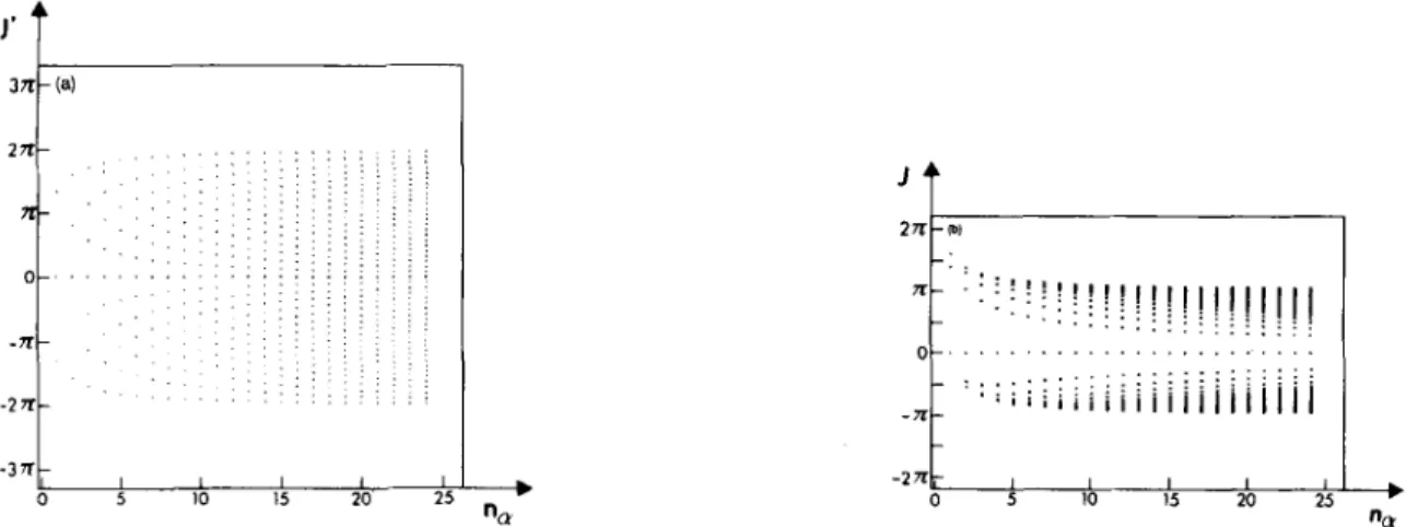
To see how rough inequalities (19a) and (19b) may be, we computed numerically some of the values of J ( p , a, y ) and

J‘(B,

LY, y). The results are shown in Figs 1-4. Each figure corresponds to a given y [i.e. (n,,, m y , i,)] of the

SV

and we plotted all

J ( p ,

a, y ) [resp. J ’ ( B , a, y ) ] allowed by selection rules (15) [resp. (16)) for each degree n, (up to degree 25

-

ny) of the

MF.

There are many J and J‘ for each nor, but we know they all satisfy inequalities (19a) and (19b) for large n,. This is of

course what we see on Figs 1-4. But the numerical results also strongly suggest there might be a bound for the J and J‘ that

-371

I I I I I

0 5 10 15 20’ 25

Figure 1. See Section 3.2. AS a function of nnr the degree of the Main Field. (a) J’ interaction integrals for n,, = 1, m,, = 0, i, = m i n e . (b) J interaction integrals for n, = 1, m y = 0, i, = cosine.

(7)

J' II- 0 -I[- -?I[-

' t

'

J ' J A .2n 2rr-lcl 2 ~ - l a l lbl . . . -. . . . . . . 1 1 I I _{- 2 n} I I I I - 2 7 - _I _I _I _I

''

t

-2nL I I I I I 0 5 10 IS 20 2s

'

n a - 3 d 0 S I 10 I IS I 20 I 25 I

'

"a

Figare 3. See Section 3.2. As a function of n,, the degree of the Main Field. (a) J' interaction integrals for n, = 2, my = 2, i, =cosine. (b) J interaction integrals for n y = 2, my = 2, i, = sine.

"t

Figure 4. See Section 3.2. As a function of n,, the degree of the Main Field. (a) J' interaction integrals for n, = 5 , my = 4, i, =sine. (b) J interaction integrals for n, = 5 , my = 4, i, = cosine.

(8)

230

G. Hulot,

J .

L .

Le

Moue1 and

J .

Wahr

does not depend on nar in other words that we have

These inequalities are not as easy to derive as inequalities (19a) and (19b). We have been able to provide a proof of (20a),

using generalized spherical harmonics. But as this proof is somehow laborious, we won’t give it here. In fact we will only need

an estimate of the root mean square (RMS) value (J(n,, y ) ) of quantities J(B, (Y, y ) and J’(B, a; y ) for a given n, and y, as

defined by m,,i,,B

I)”

121)

({

N(n,,

Y)

+“(n,,

Y)

c

[J(B,

a; Y)l”+

c

[J’(B,

a? Y)l’ m,.i,.B ( J ( n a 9 Y ) ) =

where the first summation is performed over all the N(n,, y ) possible values for ( m a , i,,

8)

from (15) and the second over all

the N’(n,, y ) possible values for (m,, i,,

B)

from (16).

The result suggested by (20) is that (J(n,, y ) ) remains finite when n, becomes large. Indeed (20) implies

In fact we can prove (see Appendix A) that one can exactly describe the behaviour of the (J(n,, y ) ) when n, becomes large

with the following formulae:

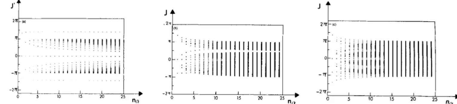
This result is in perfect agreement with the numerical results of Fig. 5. As can be easily checked, the factor

[n,(n,

+

l)]”2(n,

+

1/2)-’ is very close to 1 (it lies betweeh 0.94 and l), so that from a practical point of view, rather than (22a), we will assume

f n i f m , = ~ ,

(22b) will soon prove useful (Section 4.2 and following).

cJ’

2 %

t

n . . .

. . .

1.

0 - 5 10 15 20 25

“,

0 - 0 5 10 I5 20 25 n,

F p r e 5. See Section 3.2, formula (21). RMS values (J(n,, y ) ) of the J and J’ interaction integrals when (arr, y ) is given, as a function of n,,

the degree of the Main Field, for: (a) SV degree ny = 1; (b) SV degree ny = 2; and (c) SV degree ny = 5. In all three cases, those values lying

well above the others correspond to the special case m y = 0.

(9)

Assessing computed

flows

at the

CMB

231

(nr)

10000 35000 M O O 0 250M) 20000 15000- 1oooo 5000 -5000 -10000 4 ESTIMATION O F T H E E R RO RS O N T H E C O M P U T E D S V COEFFICIENTS D U E TO T HE TRUNCATION OF T H E E X P A N S I O N S O F T H E F L O W A N D OF T H E MF I N T H E INDUCTION EQUATION

4.1 Estimations of the field and of the flow at large degrees

The energy of the magnetic field at the CMB (within a multiplying constant) is (Lowes 1966)

A (b)

-

- - - 0 * * - 0 0 - - O A

-

- - 1 I 1 1 I 2 A 6 8 1 0 1 2

-

m 1 4 x 2

w=-

\ \ ( B . B ) ~ s =

C.

w(n,) ",=l Core with nu

W n , )

= (n, + 1)

c

[ ( b y ) ' + ( 6 3 ' 1 . m,=O

The spectrum of the main field [i.e. the collection of the W (n , ) ] is now well known. It features a slope change at degree 13

indicative of a strong crustal field for degrees greater than 13 (Langel & Estes 1982). We therefore know that it is difficult if

ever possible to infer the spectrum of the core-generated MF for degrees greater than 13. On the other hand, we know that for

degrees less than 13 the energy of the crustal field is much smaller than that of the MF [for degree 13, the contribution of the

crustal field does not exceed 20 per cent of W (Counil, Cohen & Achache 1991)], so that it is possible to assume that this part

of the spectrum is of internal origin. Fig. 6(a) shows W ( n , ) corresponding to a model of the field for the year 1980 up to

degree 13 continued to the core (Cohen & Achache 1990). (In fact any other model for the same period would give the same

figure.) One infers from this drawing that W(n,) can be considered as obeying an exponential law for large enough n,:

W(n,)

-

with k = 0.14, W, = 2 X lo1' (nT)'. (23)

It is a reasonable assumption that equation (23) describing the behaviour of the core field spectrum should remain valid for

degrees n, larger than 13.

Woe-*""= (n,

+

1)(2n,

+

l)(b(n,))'

so we have (for large n,):

For a given nu, we now define b(n,) as a random centred variable, its RMS value (b(n,)) being such that

We argue that for a given n,, the 6, MF coefficients may be viewed as independently drawn lots of the random variable b(n,).

We can indeed calculate the RMS value (b(ly)) and

the mean value

8,

of

the b,

coeficients

for each degree n, of

the

MF

model and compare them respectively to (b(n,)) from (24) and to the mathematical expectation of b(n,), E[b(n,)] = 0 (see

Fig. 6b). The agreement is fairly good, the discrepancy being easily explained by the finite number (2n,

+

1) of b, coefficients:

in the case of the mean value, for instance, we know that

6,

is allowed to fluctuate with an RMS amplitude of

( b ( n , ) ) / q m about the value E[b(n,)] = 0. Too quick a glance at Fig. 6(b) might give the uncomfortable feeling that the

lo9

I I I I I

2 4 6 8 1 0 1 2 c na

Figure 6. See Sections 4.1 and 4.2. (a) Spectrum of the magnetic field at the CMB [ W ( n , ) is in (nT)']. Also shown (solid line), the values

given by formula (23). (b) As a function of nu, the degree of the Main Field (degree 1 not shown): the RMS value ( b ( n , ) ) for the model from

&hen & Achache (1990) (stars); the mean value

6-

(open triangles); the RMS value ( b ( n , ) ) given by formula (24) (open squares); the

fluctuation 'amplitude' for

6-

(solid lines).

(10)

232

b, do not fluctuate as much as expected. Let us make a very simple reasoning in order to see if this distribution is really too

unlikely; the

b,

seem to be too often (10 times out of 12) within the RMS amplitude ( b ( n , ) ) / \ l Z - n

+

1 and too seldom above

this amplitude. If we assume that we deal with Gaussian random variables, what would most likely happen is that eight out of

the 12

6,

would be within this amplitude and four above. The probabilities corresponding to these two cases are respectively

C:, x (0.69)” x (0.31)2 = 0.155 and C:2 x (0.69)’ x (0.31)4 = 0.235, which proves that the observed case is nearly as likely to

happen as the most likely case: we may assume the b, coefficients are independent drawing lots of the random variable b(n,).

There is still another difficulty linked to this statement: since the values of the 6 , coefficients rely on the choice of the

longitude’s origin, would the statement still be true if this origin was to be shifted? This important point is discussed in

Appendix B. It is shown that (hopefully) the statement does not rely on the longitude’s origin.

G. Hulot,

J .

L. Le Moue1 and

J .

Wahr

We can define the energy of the flow in the same way as we did for the MF:

Using expansion (8), we can write

We mentioned in the introduction that, in order to obtain a practical uniqueness, the flow at the CMB must be supposed

to be large scale. This implies at least

m m

E s = E s ( n S ) < m and E , = E,(np)<m.

n a = l n p = l

In order that (26) holds we must suppose that for np large enough,

where E , is a constant we will estimate in Section 4.3. Here again we introduce a statistical formalism t o describe a typical flow (s t ) . For a given no, we will define u(np) as a random variable such that the ss and tp may be viewed as independently drawn

lots of this random variable. Not much is known a priori about u(ns) but we expect and we will assume that

E [ u ( n s ) ] = 0.

(It is easy to make sure aposteriori that this is reasonable using, for instance, the ‘typical’ flow derived in Section 5.1.) And, on

the basis of (25) and (27), we obtain for large no:

Relations (28) are used as ‘a prior? information in the inversion schemes (e.g. Backus 1988). It is worth noting that this

statistical assumption raises the same question as the statistical assumption we used for the MF: is it independent of the choice

of the longitude’s origin? The arguments developed in Appendix B in the case of the MF can easily be extended to the case of

the flow so that the answer is the same. None of the statistical assumptions we make for either the MF or the flow relies on this

choice and of course, the same thing will be true for the conclusions we will reach in this paper.

4.2 Contribution of large degree terms of the field and of the flow to the induction equation

Returning to equation (9a) we can write it in the form

m

hY

=

c

B(y,,n,)

n , = l

with

n.,

B(Y,

n,) = n,(n,

+

1)

c

b , [ s p W a:

Y)

+

% d ‘ ( B , cu,

u)l.

m,=O i b ~ ( c , s ) ,3

B ( y , n,) is the contribution of the components of the MF of degree n, to the

SV

of index y when acted by the flow (s t ) .

Equation (29) involves a priori an infinite sum on

p.

But as already mentioned for equation (21), the selection rules (15)

and (16) which apply to the J ( B , a; y ) and J ’ ( B , a, y ) and therefore to the d ( b , a, y ) and d ’ @ , a; y ) make it finite. Indeed y

being given, if we choose a large n,, it follows from (15) [resp. (16)] that the number N ( n p , y ) [resp. N’(np, y ) ] of non-zero

(11)

Assessing computed flows at the C M B 233

d(p, a, y ) [resp. d ' ( p , a, y ) ] involved in ( 2 9 k p l e a s e note that these are the same N(n,, y ) and N'(n,, y ) as those involved in

(21)-is about 2n,(n,

+

1) (resp. 2n,n,) if m y = 0, and 4n,(n,

+

1) (resp. 4n,n,) otherwise. We want to estimate the

magnitude of B ( y , n,) for large n,.

Considered from the statistical point of view we adopted for the description of the MF and of the flow, (29) is the

summation of products of independent draws of several random variables [for instance by,&, by' and by,& are three

independent draws of the same random variable b(n,), and b(n,), b ( n b ) and u ( n s ) are independent random variables; the

assumption that u(n S) and b(n,) are independent variables could be discussed. But to know whether it holds exactly is not

important for the order of magnitude calculation we want to make in this paper: the interactions between the flow and the field

are so complex that it would require vkry sophisticated correlations between u ( n s ) and b(n,) for these interactions to act in a

coherent manner and significantly change our results]. Then, recalling that E [ b ( n , ) ] = 0 and E [ u ( n s ) ] = 0, we have from (29):

From (17) and (28) we know that for n, large compared to n, (.(.a)>

-

(4n,))*

This allows us to write, also using (11) and (22b),

The previous considerations provide a statistical estimate for the magnitude of B ( y , na). For n, large compared to ny

(31b) becomes [recall (7), (24), (28) and (22a)l

(B(K a,)) - g ( y ) B o B ( n J (314

with

where g ( y ) describes the dependence on the degree of the created SV, B(n,) the dependence on the degree of the MF, and B ,

has the dimension of a SV.

Let us turn now to the core of the problem. Define what we ought to call the 'rest of the SV', i.e. the summation of all the

B ( y , n,) that have been neglected because of the truncation (Section 2):

R(y,N,)=

c

B ( y 7 n a ) .

n , = N , + l

The 'rest of the SV' will be our means to measure the error on the computed SV coefficients due to the truncation of the

expansions of the flow and the MF in the induction equation. To evaluate R ( y , N,), we will go on using the statistical

formalism already introduced. The assumptions made about the statistical independence of the b(n,) and the u(nS) allow us to

treat the different B ( y , n,) as also statistically independent. From (30) we then have

E"Y9

m1=

0

and

1 12

(W?

Nu))

-

(

2

( B ( y , n,))')

na=N,+l

and using (31c), this can be written

Thus equation (32) provides a statistical answer to our question.

showed this is compatible with the data, it might not exactly be the case. As one can see on Fig. 6(b), stating

The above result has been derived assuming among other things that E [ b ( n , ) ] and E [ u ( n s ) ] are zero. Although we

E[b(n,)l= Eb(n,)(b(n,)) (33)

(12)

234

where Eb(n,) has a constant Eb absolute value and a random sign (function of n,) and assuming that eb is not larger than say

0.2, is as plausible a statement as E [ b ( n , ) ] = 0. In the same way, rather than assuming E ( [ u ( n s ) ] = 0, we could as well assume

G.

Hulot,

J .

L.

Le Mouel and

J .

Wahr

where e,(np) also has a constant E, absolute value and a random sign (now function of no); can be supposed smaller than

say 0.3 from the ‘typical’ flow derived in Section 5.1. Fortunately such corrections will not affect the result (32), as is shown in Appendix C.

We now have a value at our disposal to evaluate the SV error R ( y , N,) due to the truncation of the induction equation.

4.3 Numerical results

In this section we will derive some numerical values for the ( R ( y , N,)). To do so, we need some values for the not yet known

parameters E, and 1. Recalling (27), we note that the value of E , depends on the value chosen for 1, in other words E, = Eo(Q

On the basis of a number of published models of the flow at the CMB (Le Mouel et al. 1985; Voorhies 1986; Gire, Le Mouel &

Madden 1986; Whaler & Clarke 1988; Bloxham 1989; Bloxham et al. 1989; Gire & Le Mouel 1990), a fair way of defining the

value of E,(l) is to make sure that

Ed’)

10-6 rad2 yr-2

E(ns = 10) =

-

10’

It remains to choose the value of the rather arbitrary parameter 1. A standard value for 1 is 2 (Backus 1988; Gire & Le

Moue1 1990), but we also made the calculation for 1 = 3 and 1 = 1.1 in order to explore the effect of the choice of 1.

Eventually we need the truncation degree N , of the MF. This value is directly given by the observation: N , = 13, since 13

is the maximum degree (because of the crustal field) we can reasonably resolve for the MF. We therefore present three sets of

results, (1, N,) being: (1.1,13), (2,13) and (3,13). Table 1 gives the numerical values of g ( y ) , showing its evolution with the

degree n,, of the SV. Table 2 illustrates the fact that the value of our estimation for R ( y , N,) is fairly independent of the value

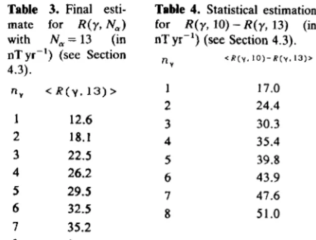
we choose for 1. For this reason we will keep 2 as a reasonable value for 1. Table 3 then gives our final estimate for R ( y , N,)

with N , = 13.

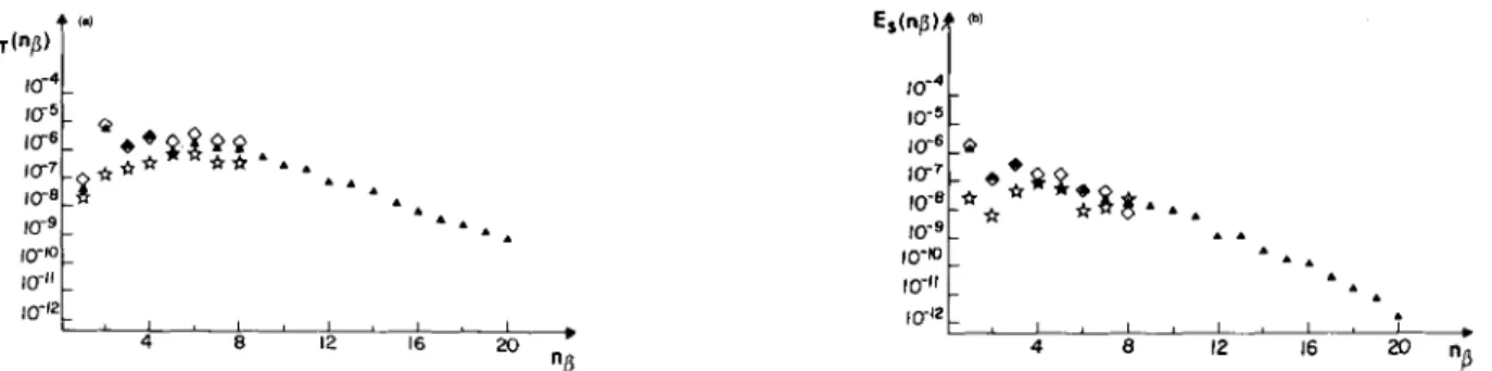
Because the calculation that led to formula (32) is based on the use of asymptotic expressions, we would like to confront

our result with some kind of ‘real’ data. Of course we do not have the data that would enable us to confront the true R ( y , N,)

with our estimation ( R ( y , N , ) ) . But it is nevertheless possible to assess the validity of our approach. Using the typical model

for the flow (Section 5.1) and a model of the main field (e.g. Cohen & Achache 1990), we can easily calculate the contribution

to the SV of the field components of degrees 11 to 13, i.e. the ‘real’ R ( y , 10) - R ( y , 13). Using the same statistical approach as

the one used to derive ( R ( y , N , ) ) , we can make a statistical estimation of this difference, ( R ( y , 10)

-

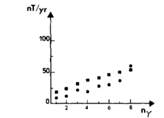
R ( y , 13)) (see Table 4).

Fig. 7 shows both the ‘real’ RMS value of R ( y , 10) - R ( y , 13) and the RMS statistical estimation ( R ( y , 10)

-

R ( y , 13)). Our

statistical estimation is in fairly good agreement with the ‘real’ case. We therefore consider formula (32) as a realistic

estimation for R ( y , N,).

Table 1. g ( y ) Table 2. Dependence of ( R ( y , 13))/g(y)

(equation 31) as a

function of the SV 1 - 1 . 1 1 = 2 1 - 3

with I (in nT yr-’) (see Section 4.3).

19.4 15.2 degree ny (see Section 4.3). < R ( v . 1 3 ) > / g ( ~ ) 24.6 n” d Y ) 1 0.650 2 0.932 3 1.158 4 1.350 5 1.520 6 I .674 7 1.815 8 1.947

Table 3. Final esti-

mate for R ( y , N,)

with N, = 13 (in

nT yr-’) (see Section

R, <R(y.13)> 4.3). 1 12.6 2 18.1 3 22.5 4 26.2 5 29.5 6 32.5 7 35.2 8 37.8

Table 4. Statistical estimation

for R ( y , 10) - R ( y , 13) (in nTyr-’) (see Section 4.3).

‘ R ( y . I O ) - R ( y . 1 3 ) > R V 1 17.0 2 24.4 3 30.3 4 35.4 5 39.8 6 43.9 7 47.6 8 51.0

(13)

Assessing computed

flows

at the

C M B

235 t

Figure 7. See Section 4.3. As a function of ny, the SV degree: the 'real' RMS value of R ( y , 10) - R ( y , 13) (full circles); the W S statistical

estimation ( R ( y , 10) - R ( y , 13)) (full squares).

4.4 Implications for the calculation of the flow at the CMB

We now need to compare ( R ( y, N,)) to the

6,

coefficients of the SV. This is the purpose of Fig. 8(a) which shows ( R ( y , N , ) )

together with the RMS value of the

6,

(at the CMB) as a function of n,. The most important result is that the truncation errors

lie well below the RMS values of the b y . This proves that the principle of deriving a flow (within the assumed hypothesis) using

an unavoidably truncated expansion of the field has not to be questioned. But it does not mean that the error is negligible and

its estimation of no interest. Thanks to this estimate we are indeed able to give some indications on which part of the flow

could ultimately be resolved from the magnetic data.

Considering the truncated form of equation (9b) (Section 4.2): Nu

b y = B ( y , n , ) with N,=13,

n,=l

and recalling that the SV is hardly known for ny greater than 8, we know that only the degrees of the flow less than 21 will be

constrained by (9c) (i.e. by the data). Of course, not all degrees of the flow will be constrained in the same way: the greater the degree, the poorer the constraint.

Define B ( y , n,, No), the contribution to B ( y , n,) of the degrees of the flow greater than a given degree No:

n,

W Y ,

n,, N,) = n,(n,

+

1)

2 C

2

b , [ + ( ~ , a;

v)

+ t , d ' ( ~ ,

r)I

m,=O i u E ( c . s) f3'

/3' meaning

B

such that n, > N,, and

N.

R(y, N,, N,) =

c

B(Y, n,, Np)

n u = l

the contribution to

6,

in (9c) of the flow components with degree greater than N,.

We can make a statistical estimation of B ( y , n,, N,) and R ( y , N,, N,) in the way we did for B ( y , n,) and R ( y , N,). We will

use the same hypothesis for the field and the flow as previously but we won't need any asymptotic estimation for the J and J'

(only a finite number of them are involved in the calculation). We obtain for the RMS value of B ( y , n,, N,):

1 12

ny(nu + 1)

llTy

112

m,=O i,E (CJ)

@(Yl n,, N , ) ) =

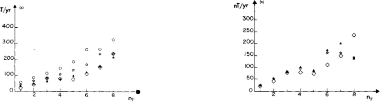
F i e 8. See Section 4.4. As a function of ny, the SV degree: (a) the RMS value of the by at the CMB (crosses): the ( R ( y , N, = 13)) (open

diamonds); (b) the ( R ( y , N, = 13)) (open diamonds); the RMS value of the ( R ( y , N, = 13, N, = 13)) over the several possible my (the

( R ( y , N,, N,)) have little dependence on m y ) (full triangles); same for the ( R ( y , N, = 13, N, = 12)) (open stars).

(14)

236 G . Hulot, J .

L. Le Moue1 and

J .

Wahr

and for the RMS value of R ( y , N,, N,):

Recalling (24) and (28), (35) allows us to calculate ( R ( y ,

N,,

N B ) ) for any given N,.

We now simply argue that if ( R ( y ,

N,, N,))

is less than or of the order of the truncation error ( R ( y , N , ) ) , the magnetic

are unable to constrain the components of the flow of degree greater than Ns. We made the calculation for various N, of

interest and Fig. 8(b) shows our results. As can be seen, ( R ( y , N , = 13, N, = 13)) is always less or about the size of

( R ( y , N, = 13)) whereas ( R ( y ,

N,

= 13,

N,

= 12)) is already quite comparable to or even larger than ( R ( y , N, = 13)).

The conclusion is that the error due to the truncation of the expansion of the field makes it impossible to derive any

information on the degrees of the flow greater than 12. As a pleasant consequence this however proves that we may truncate

the expansion of the flow at degree 12 before inverting equation (14).

5 DERIVING THE FLOW A T T H E CMB: A SIMPLE E V A L U A T I O N OF T H E

PRESENT-DAY

ACCURACY

The previous study was made assuming that the only errors that were allowed to creep in the calculation were those linked to

the truncation of the expansions. This gave us a hint of what information could ultimately be extracted from the magnetic data

in the case the Gauss coefficients by would be perfectly known. Unfortunately, such is not the case. We must take this

important fact into account to clarify what can be said about the flow with the present-day magnetic data. 5.1 The error on the SV data

It is not an easy task to evaluate the errors that are made on the by in the process of deriving a model of the SV from the

observations. But for the following discussion, we will assume that comparing two available models for the year 1980 [i.e.

computing the differences Ab,, = b,,(USGS80) - b,,(GSFC80) between the USGS80 SV coefficients (Peddie & Fabian0 1982a)

and the GSFC80 SV coefficients (Langel, Estes & Mead 1982)] is good enough a way to have estimates of these errors.

Although this approach is probably not the best one, it is in good agreement with the results of Langel et at. (1986) who find

errors on

by

(qualified as ‘crude estimations’) which are slightly smaller than our estimates for degrees 1 to 4 but are

comparable to those estimates for larger degrees. We also find a good agreement of the map of the difference between the

USGS80 and CSFC80 models (not shown here) with the maps of Barker 22 Barraclough (1985) showing the error one can

expect

for

any SV model because of the non-uniform geographic distribution of the magnetic measurements. Eventually, our

evaluation is in good agreement with the conclusions of Barraclough (1990) and Lowes (1990). We therefore take our

estimation as good enough for this study.

5.2

The

part of the flow that is constrained by the present-day data

We now follow the same reasoning as in Section 4.4, but, instead of comparing ( R ( y , N,, N,)) with ( R ( y , Na)), we will

compare ( R ( y , N,, N,)) with (b,(USGS80)

-

b,(GSFC80)), the RMS value of the b,(USGS80)

-

6,(GSFC80) for a given

degree n,, of the SV, and conclude that if N, is such that ( R ( y , N,, N,)) is smaller than b,(USGSSO)

-

b,,(GSFC80)), then the

components of the flow of degree larger than N, are not at all constrained by the data. Fig. 9(a) illustrates the study we made

nT’yr

T

la’

:::I

200

looL

0 0 0 t I , , , , , 2 4 6 0 ? 1 nr 0 8 $ b

Figure 9. See Section 5.2. As a function of n y , the SV degree. (a) The RMS value (6,(USGSSO)

-

b,(GSFC80)) (open diamonds); the RMS value of the ( R ( y , N, = 13, N, = 8)) over the several possible m y (full triangles); same for the ( R ( y , N, = 13, N, = 7)) (open stars); same for the ( R ( y , N, = 13, No = 6)) (open circles), (b) The RMS value (b,(USGSBO)

-

bJGSFC80)) (open diamorrds); the RMS value (b,(USGS80) - b,((typical flow)), where the b,(typical flow) aFe the coefficients of the SV created by the ‘typical’ flowsee text (open stars);

the RMS value (bJUSGS80) - b,,(second flow)), where the b,(second flow) are the coefficients of the SV created by the second flowsee

text (full triangles).

(15)

Assessing computed flows at

the C M B

231 following this criterion. It clearly comes out that the degrees of the flow larger than 8 are not at all constrained by the present SV data.

In order to evaluate more precisely the accuracy of the components of the flow with degree 1 to 8, we will derive a first, explicit model of the flow. B'ecause the 1980 Main Field is very well defined (thanks to MAGSAT data) we decided to make our computation for the year 1980. We assume the flow is geostrophic (we use the tangentially geostrophic basis). Although, as already mentioned, this is not a key point (see the remark at the end of the section), the following results will therefore preferentially apply to geostrophic motions. The calculation is very similar to those done by Gire & Le Moue1 (1990) and

(a,

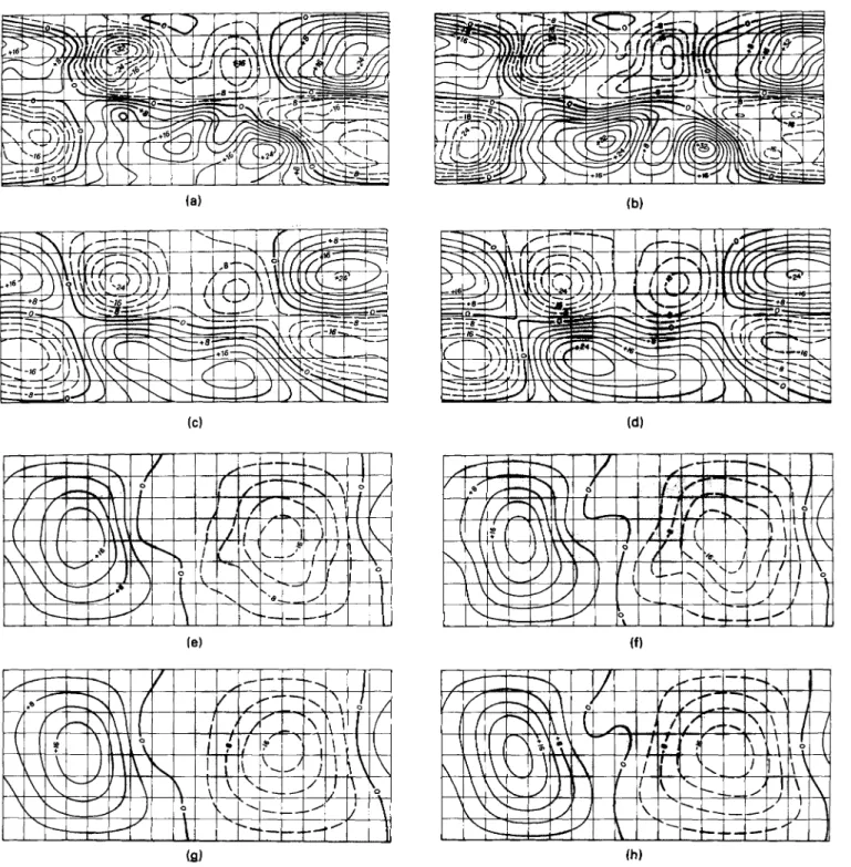
Figure 10. See Section 5.2. Scale: 10-4radzyr~'. Parallels are shown every 20" between -80" and 80" and meridians are shown every 20°,

Greenwich meridian being at the centre of the picture. Dashed lines for negative values, full lines for positive values. (a) Toroidal scalar of the 'typical' flow (see text). (b) Toroidal scalar of the second flow (see text). (c) Toroidal scalar of the 'typical' flow truncated at degree 4. (d) Toroidal scalar of the second flow truncated at degree 4. (e) Poloidal scalar of the 'typical' flow. (f) Poloidal scalar of the second flow. (g) Poloidal scalar of the 'typical' flow truncated at degree 4. (h) Poloidal scalar of the second flow truncated at degree 4.

(16)

238

G. Hulot, J . L .

Le

Mouel

and J . Wahr Hulot, Le Mouel & Jault (1990):

(i) the flow is calculated up to degree 20, order 19;

(ii) the energy of the flow is required to converge in the way described in Section 4.1 [recall (27)] with I = 2;

(iii) the SV created by the calculated flow is required to fit the USGS80 SV model within the error previously defined; and

(iv) the MF model (up to degree 13) is taken from Cohen & Achache (1990).

Since we just proved that the components of the flow of degree larger than 8 cannot be determined, this flow is definitely

not the flow occurring at the CMB: we can feel fairly confident about the lowest degrees components of the computed flow

(within the limit we are going to explore next) whereas we can only say that the high-degree components are acceptable (i.e.

complying with all our a priori requests). We will refer to this flow as a 'typical flow' (this is the flow we referred to in Sections

4.1, 4.2 and 4.3).

For the reasons developed above we argue that a second equally valid flow may be obtained by truncating a priori the flow

at degree 8 and using another satisfying (within the error defined in Section 5.1) SV model. We decided to use the USGS80 SV

model up to degree 6 and to set all the coefficients of degree 7 and 8 to 0 [the errors for these coefficients are of the same size as the coefficients themselves: compare Fig. 9(a) to Fig. 8(a)].

According to the preceding discussion, the difference between the SV created by this second flow (as well as the one

created by the 'typical' flow) and the USGS80 SV should not be larger than the difference between the two SV models. Fig.

9(b) shows that this is indeed the case. Hence, comparing this second acceptable flow with the 'typical flow' gives us a hint of

the accuracy we can expect for the flow at the CMB when using the available magnetic data.

Figure 10 shows the maps of the toroidal and poloidal scalar of both flows. To underline the very strong similarities

existing between these flows for low-degree components, we also show the maps we obtain if we truncate them at degree 4. A

more quantitative way of comparing these two flows is to look at their spectra and at the spectrum of their difference (Fig. 11).

It appears that the energy of both flows are very similar and almost identical for degrees 1 to 4, and that the energy of the

difference is always smaller than the energy of both flows (by a factor of about 10 in the case of degrees 1 to 4), which confirms

what was seen on Fig. 10.

We therefore conclude that, whereas we cannot resolve the flow for degrees larger than 8, and despite the fact the

accuracy is poor for degrees 5 to 8 (Fig. 11; this is especially true for the poloidal component, but it is a consequence of the

geostrophic assumption that the poloidal component be less energetic than the toroidal component), the components of the

flow of degrees 1 to 4 are fairly well known. More precisely, if we introduce us(no) and u,(ns), the RMS errors on the sg and

ts, we have [recall (25)]

One should have this conclusion in mind when dealing with the different maps or figures a number of authors have

produced for the flow at the CMB. In particular, the components of degree larger than 8 d o not rely on the data but on a priori

information. So, in order to compare two different flow models, one should truncate them at least at degree 8 if not at degree

4. Let us give two typical examples. A rather common way of testing the geostrophic assumption is to compute a flow using

basic constraints (the convergence of the energy) and see whether it does or does not have the equator-nocrossing geostrophic

property (Benton 1985). But this property must be tested on large scales: a local crossing cannot be considered as significant

(Bloxham 1989). As a second example, we recall a recent study by Gire & Le Mouel (1990) who, in the purpose of establishing

some symmetry properties, used among other arguments the fact that a part of the flow 'showed no tendency to converge' (see

their Fig. 5). We can now state that this is the result of some kind of uncontrolled a priori constraint (in fact a constraint on the

energy which was awkwardly imposed in the numerical programs). It is possible to make this part of the flow converge [see Fig.

10-1' 10-12 1 e I , I , I . 1 12 16 20

'

4 8 "P 10"' 10-'2 I , I , I , I , I 12 16 20 ni 4 8

F i r e 11. See Section 5.2. As a function of no, the flow degree, the energy [units in (rad ~ r - ~ ) ' ] of the 'typical' flow-see text (MI triangles);

the second flow-see text (open squares); the difference between the typical and the second flow (open stars). (a) Toroidal components. (b)

Poloidal components.

(17)

Assessing

computed flows at the

C M B

239

ll(b) versus their Fig. 51. We however insist that this does not question the main result of their study that the flow has some

very interesting symmetry properties [confirmed and further studied by Hulot et al. (1990)l.

R E M A R K

In the main part of this study, we assumed the flow is large scale with no a priori correlation between the different components

nor any a priori constraint on the toroidal or poloidal part (recall Section 4.1). But one usually imposes some further

constraints on the flow, as mentioned in the Introduction. These are the toroidal, the tangentially geostrophic or the steady

motion constraint. It is thus of some importance to see whether these further constraints d o or do not affect our study.

Let us assume the flow is purely toroidal. As a consequence the poloidal coefficients so vanish in (29). This is equivalent to

the statement that the J’ interaction integrals be zero, and amounts to divide the value given by (31c) by a factor of about

~.

At the same time, to keep the same value for the a priori energy of the flow, ( u(np)) has to be increased by the same factor.

These two effects balance, so that nothing has to be changed in our final results [formulae (32) and (35)]. If we now assume

that the flow is tangentially geostrophic, the situation seems more tricky since this assumption introduces correlations between

the toroidal and the poloidal components of the flow. This case could be treated exactly. But taking advantage of the fact that,

for large degrees, the tangentially geostrophic flow is nearly toroidal, it is easy to show that the results are very similar to those

we obtained. As for the steady motion constraint, it amounts to using equation (3) at different epoches to constrain the steady

flow. Our analysis can be applied to each epoch so that the formulae (32) and (35) still hold.

6 CONCLUSIONS

In this paper our concern was again to try and give some qualitative and quantitative answers to the question: what can be said

about the flow at the CMB from magnetic data collected at the Earth’s surface? The question is easy to state but covers a great variety of different aspects. One immediately thinks of the validity of the frozen flux theorem, of the adequacy of modelling the

mantle as an insulator or of the fundamental ambiguity, three points that are at the very basis of the method. While not

neglecting the importance of these three points, we could fear a greater obstacle might come from other important aspects of

the problem such as the errors in the SV models or the less obvious errors linked to the unavoidable truncations of the MF and of the motion.

We showed that these two shortcomings impose some serious limitations on what can be said about this flow. On one

hand, because the accuracy of the 1980 SV model coefficients gradually worsens with the degree to the point that coefficients

with degree larger than 6 are actually unknown, the only components of the flow that can be trusted (within the frame of the

usual hypothesis: frozen flux; insulating mantle; toroidal, tangentially geostrophic or steay flows) are those with degree less

than 4 or 5 . On the other hand, our study of the errors linked to the truncation of the MF showed that, had we known perfectly

the

SV,

the flow could have been calculated for degrees as large as 12. This tends to prove that quite some improvement might

be expected by increasing the quality of the SV models. More specifically, one can aim at reducing the errors in the SV models

to the level of the errors linked to the truncation of the field. As one can see when comparing Fig. 8 to Fig. 9, the accuracy

for

degree 1 is already good enough and the accuracy for degree 2 only needs an improvement by a factor of 2 to meet this

condition. On the contrary, a lot of improvement is still needed for larger degrees. In the case of degree 8 for instance, the aim

would be to get an error as low as 0.15 nTyr-’ (at the Earth’s surface). This is a very low value one might not be ever able to

reach because essentially of the difficulties encountered in separating the external from the internal magnetic signals. But there

is no doubt some improvement is possible in the future. Let us make some simple suggestions. The SV models built to apply

the IGFW 1980 label were intended to be predictive. They suffer the noticeable inconvenience of being extrapolations of past

data-for instance the USGS80 SV model has been constructed on the basis of 1976 to 1981 data in order to predict the field

from 1980 to 1985 (Peddie & Fabiano 1982b). Such is not the case for models more specifically constructed for the study of the

Earth’s core (Langel et al. 1986; Bloxham & Jackson 1989) for which the authors interpolate rather than extrapolate the data.

Unfortunately none of these models uses data more recent than 1981 so that they do not describe the 1980 SV better than the USGS80 model. Were they extended to more recent data, an improved 1980 SV model could certainly be constructed. As for future SV models, any mean of increasing the number of data (at best covering the Earth’s surface) would be very valuable:

magnetic satellites or an implemented array of observatories such as INTERMAGNET.

In any case, let us emphasize that, even in the present day situation, low-degree terms of the flow (those with degree less

than, say, 5) are fairly well known (within the quoted basic hypothesis).

ACKNOWLEDGMENTS

This work was supported by Institut National des Sciences de I’Univers (INSU), DBT program Geodynamique Globale. IPGP

contribution No. 1181.