El Niño in a changing climate: a multi-model study

HAL Id: hal-00298272

https://hal.archives-ouvertes.fr/hal-00298272

Submitted on 13 Oct 2005

HAL is a multi-disciplinary open access

archive for the deposit and dissemination of

sci-entific research documents, whether they are

pub-lished or not. The documents may come from

teaching and research institutions in France or

abroad, or from public or private research centers.

L’archive ouverte pluridisciplinaire HAL, est

destinée au dépôt et à la diffusion de documents

scientifiques de niveau recherche, publiés ou non,

émanant des établissements d’enseignement et de

recherche français ou étrangers, des laboratoires

publics ou privés.

G. J. van Oldenborgh, S. Y. Philip, M. Collins

To cite this version:

G. J. van Oldenborgh, S. Y. Philip, M. Collins. El Niño in a changing climate: a multi-model study.

Ocean Science, European Geosciences Union, 2005, 1 (2), pp.81-95. �hal-00298272�

www.ocean-science.net/os/1/81/ SRef-ID: 1812-0792/os/2005-1-81 European Geosciences Union

Ocean Science

El Ni ˜no in a changing climate: a multi-model study

G. J. van Oldenborgh1, S. Y. Philip1, and M. Collins2

1_{Royal Netherlands Meteorological Institute, P.O. Box 201, 3730 AE De Bilt, The Netherlands} 2_{Hadley Centre for Climate Prediction and Research, Met Office, Exeter, UK}

Received: 18 May 2005 – Published in Ocean Science Discussions: 10 June 2005

Revised: 1 September 2005 – Accepted: 21 September 2005 – Published: 13 October 2005

Abstract. In many parts of the world, climate projections

for the next century depend on potential changes in the prop-erties of the El Ni˜no – Southern Oscillation (ENSO). The current staus of these projections is assessed by examining a large set of climate model experiments prepared for the Fourth Assessment Report of the Intergovernmental Panel on Climate Change. Firstly, the patterns and time series of present-day ENSO-like model variability in the tropical Pacific Ocean are compared with that observed. Next, the strength of the coupled atmospheocean feedback loops re-sponsible for generating the ENSO cycle in the models are evaluated. Finally, we consider the projections of the mod-els with, what we consider to be, the most realistic ENSO variability.

Two of the models considered do not have interannual variability in the tropical Pacific Ocean. Three models show a very regular ENSO cycle due to a strong local wind feed-back in the central Pacific and weak sea surface temperature (SST) damping. Six other models have a higher frequency ENSO cycle than observed due to a weak east Pacific welling feedback loop. One model has much stronger up-welling feedback than observed, and another one cannot be described simply by the analysis technique. The remaining six models have a reasonable balance of feedback mecha-nisms and in four of these the interannual mode also resem-bles the observed ENSO both spatially and temporally.

Over the period 2051–2100 (under various scenarios) the most realistic six models show either no change in the mean state or a slight shift towards El Ni˜no-like conditions with an amplitude at most a quarter of the present day interan-nual standard deviation. We see no statistically significant changes in amplitude of ENSO variability in the future, with changes in the standard deviation of a Southern Oscillation Index that are no larger than observed decadal variations.

Correspondence to: G. J. van Oldenborgh

(oldenborgh@knmi.nl)

Uncertainties in the skewness of the variability are too large to make any statements about the future relative strength of El Ni˜no and La Ni˜na events. Based on this analysis of the multi-model ensemble, we expect very little influence of global warming on ENSO.

1 Introduction

The El Ni˜no – Southern Oscillation phenomenon (ENSO) is the largest and best known mode of climate variability that affects weather, ecosystems and societies in large parts of the world. The influence of increasing greenhouse gases on the properties of ENSO is a critical question in determining the impacts of climate change at the regional scale. Because of the complexities of the physical processes involved, we must rely heavily on complex climate models which repre-sent interactions between those processes explicitly. Here we assess ENSO simulations in the multi-model ensemble col-lected for the Intergovernmental Panel on Climate Change (IPCC) Fourth Assessment Report (4AR).

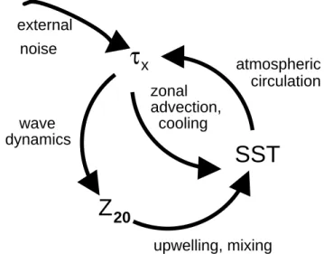
Observations and understanding of ENSO have progressed rapidly over the last decade (e.g. McPhaden et al., 1998; Neelin et al., 1998). The theoretical framework we will be using is sketched in Fig. 1 (Fedorov and Philander, 2001; Burgers and van Oldenborgh, 2003). The main positive feed-back in the ENSO cycle is represented by the outer loop (Bjerknes, 1966). Wind anomalies in the central equatorial Pacific generate thermocline anomalies which travel to the east. In the eastern equatorial Pacific these upwell as sea sur-face temperature (SST) anomalies, which in turn give rise to wind anomalies in the central Pacific. There is a sec-ondary feedback loop in the central Pacific (Wyrtki, 1975; Picaut et al., 1996), whereby SST is affected directly by wind anomalies via advection, anomalous upwelling, evaporation and mixed-layer depth anomalies. These central Pacific SST anomalies in turn influence the wind. The whole system is

SST

advection,

cooling

upwelling, mixing

wave

dynamics

τ

_x

zonal

atmospheric

circulation

Z

₂₀

external

noise

Fig. 1. The main feedbacks in the ENSO cycle.

close to stability and affected by external noise in the form of wind variations. While this conceptual model represents radiative feedbacks (Yu and Boer, 2002) only as damping terms, we should note the climate models examined all have complex representations of clouds and radiation.

Most climate models now show ENSO-like oscillations in the tropical Pacific and the properties of the modeled time series in the current climate may be compared with that ob-served. However, there are many different physical ways in which models can produce interannual oscillations. Using the ENSO theory outlined above, we first evaluate whether the main nodes in Fig. 1 have the correct variability. Next, we compare the strength of the couplings in the models to the the observations. The changes in ENSO properties under global warming can then be assigned confidence levels using these findings.

Previous complex model studies (e.g. Meehl et al., 1993; Knutson et al., 1997; Tett, 1995; Timmermann et al., 1999; Collins, 2000a,b) have used a wide range of techniques to evaluate the model ENSO behaviour and found a wide range of responses to increasing greenhouse gases from no change to significant changes in the amplitude, frequency and skew-ness of ENSO. As an example of more recent work in the manner of the study we present here, Zelle et al. (2005) anal-ysed the links of the feedback chains quantitatively in the NCAR CCSM 1.4 model. They found that in spite of very reasonable overall ENSO properties, this coarse resolution model suffers from a number of flaws that cast doubt on the projected ENSO properties: the wind response is too narrow in latitude leading to a more stable ENSO cycle; the wind re-sponse does not depend on the background temperature, and the central Pacific surface cycle is too strong compared with the Bjerknes feedback loop. By examining the key physi-cal processes responsible for ENSO properties in the mod-els, we can build confidence in their predictions of changes

in properties in a warmer world. Ultimately we should attach formal likelihoods to different model projections in order to make probabilistic predictions of future climate (e.g. Murphy et al., 2004).

The outline of this article is as follows. First, the models and their output are introduced in Sect. 2. For these models we consider the overall ENSO properties: amplitude, pattern, spectrum of the time series in SST in Sect. 3 and the corre-sponding amplitudes in zonal wind stress and thermocline depth in Sect. 4. Next, we discuss the wind response to SST anomalies in Sect. 5 and the SST response to thermocline and wind anomalies in Sect. 6. The response to increasing greenhouse gases is discussed in Sect. 7 and we give a short set of conclusions in Sect. 8.

2 Models

The model set consists of the climate models that had made enough data available via the IPCC data center at PCMDI on 15 April 2005 (subsurface data for ECHAM5/MPI-OM and UKMO HadGEM1 was obtained directly from the modeling groups). The list is given in Table 1, including references to detailed information about the models. Properties of present-day ENSO are from the “Climate of the twentieth cen-tury” (20c3m) experiments except for the UKMO HadGEM1 model, for which the pre-industrial control (picntrl) was used. For the future climate we used the last 50 years of the SRES A2 experiments, except for FGAOLSg-1.0 and MIROC3.2 (hires), for which the SRES A1B was used, and GISS-EH and UKMO HadGEM1, which only had “1% in-crease per year to doubling” (1pctto2x) experiments avail-able.

Observations are mainly taken from the Tropical Atmo-phere Ocean (TAO) array of moored buoys (McPhaden et al., 1998), which has measured many variables at a relatively coarse grid. Most buoys have been deployed in the late 1980s, so that the length of the record is the main restric-tion. SST measurements go further back, the pattern of ENSO variations is compared to the SSTOIv2 analyses of Reynolds et al. (2002) over 1981–2004 and the time series properties are evaluated against the reconstruction of Kaplan et al. (1998) which covers the period 1856–2003. Finally, we use the NCEP tropical Pacific ocean reanalysis 1980–1999 (Behringer et al., 1998) for subsurface temperatures and the ERA-40 reanalysis (Uppala et al., 2005) for sea-level pres-sure (SLP) and zonal wind stress (τx).

3 SST variability in the tropical Pacific

Most of the climate models considered show ENSO-like os-cillations in the tropical Pacific. We compare the SST ex-pression of these oscillations in the current climate with that observed by calculating the first EOF over the region

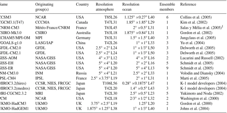
Table 1. The models considered here. The ocean resolution is the resolution along the equator. The number of ensemble members refers to

runs with different initial conditions. For most models, ocean data was available only for a single ensemble member.

Name Originating Country Resolution Resolution Ensemble Reference group(s) atmosphere ocean members

CCSM3 NCAR USA T85L26 1.125◦×0.27◦L40 6 Collins et al. (2005) CGCM3.1(T47) CCCMA Canada T47L31 1.85◦×1.85◦L29 1 Kim et al. (2002)

CNRM-CM3 M´et´eo-France/CNRM France T63L45 2◦×0.5◦L31 1 Salas y M´elia et al. (2005)1 CSIRO-Mk3.0 CSIRO Australia T63L18 1.875◦×0.84◦L31 1 Gordon et al. (2002) ECHAM5/MPI-OM MPI Germany T63L31 1.5◦×1.5◦L40 3 Jungclaus et al. (2005) FGOALS-g1.0 LASG/IAP China T42L26 1◦×1◦L33 3 Yu et al. (2004) GFDL-CM2.0 GFDL USA 2.5◦×2◦L24 1◦×1/3◦L50 3 Delworth et al. (2005) GFDL-CM2.1 GFDL USA 2.5◦×2◦L24 1◦×1/3◦L50 3 Delworth et al. (2005) GISS-AOM NASA/GISS USA 4◦×3◦L12 4◦×3◦L16 2 Lucarini and Russell (2002) GISS-EH NASA/GISS USA 5◦×4◦L20 2◦×2◦L16 5 Schmidt et al. (2005) GISS-ER NASA/GISS USA 5◦×4◦L20 5◦×4◦L13 9 Schmidt et al. (2005) INM-CM3.0 INM Russia 5◦×4◦L21 2.5◦×2◦L33 1 Volodin and Diansky (2004) IPSL-CM4 IPSL France 2.5◦×3.75◦L19 2◦×1◦L31 1 Marti et al. (2005)

MIROC3.2(hires) CCSR, NIES, FRCGC Japan T106L56 0.28◦×0.1875◦L47 1 K-1 model developers (2004) MIROC3.2(medres) CCSR, NIES, FRCGC Japan T42L20 1.4◦×0.5◦L43 3 K-1 model developers (2004) MRI-CGCM2.3.2 MRI Japan T42L30 2.5◦×0.5◦L23 5 Yukimoto and Noda (2002) PCM NCAR USA T42L18 2/3◦×1/2◦L32 2 Washington et al. (2000) UKMO-HadCM3 UKMO UK 3.75◦×2.5◦L19 1.25◦L20 2 Gordon et al. (2000) UKMO-HadGEM1 UKMO UK 1.875◦×1.25◦L38 1◦×1/3◦L40 1 Johns et al. (2004)

1_{Salas y M´elia, D., Chauvin, F., D´equ´e, M., Douville, H., Gueremy, J. F., Marquet, P., Planton, S., Royer, J. F., and S., T.: Description and}

validation of the CNRM-CM3 global coupled model, Climate Dyn., submitted, 2005.

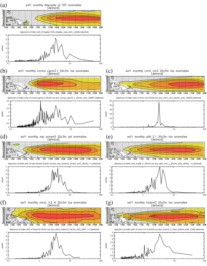
10◦_S–10◦_{N, 120}◦_E–90◦_{W, as this captures the main} pat-tern, period and amplitude of SST variability. It excludes the coastal El Ni˜no which models do not simulate, presumably because the thermocline is too deep as a consequence of the absence of stratus clouds. Despite this limitation, the char-acteristic examples shown in Fig. 2 show that many models can capture SST variability well.

In Table 2 the main features are summarized for all mod-els. In the SSTOIv2 analysis (1981–2004) the first EOF ex-plains 65% of the variance and matches the cold tongue up-welling region along the equator (Fig. 2a). The correspond-ing time series of the Kaplan analysis (1856–2003) has a broad peak in the spectrum spanning periods from 2.5 to 6 years. The standard deviation is 0.20 (with the EOF pattern normalized to one) and the skewness is 0.54; this means that SST anomalies are in general larger during El Ni˜no than dur-ing La Ni˜na.

The GISS-AOM and GISS-ER models do not appear to simulate any ENSO variability and are not considered in the rest of the paper. This is most likely due to the ocean resolu-tion being too coarse to describe the equatorial wave guide. We should note however that other coarse resolution mod-els can simulate some ENSO variabiliy (Collins, 2000b) and that the highest ocean resolution does not guarantee the best simulation by this measure.

In the models CCSM3 (Otto-Bliesner and Brady, 2001) and CGCM3.1(T47) the SST variability pattern is displaced to the west, the peak in the spectrum is at slightly higher frequencies than in the observations, the amplitude is lower than observed and the skewness close to zero (e.g. Fig. 2b). These are well-known (but not fully understood) effects of a coarse-resolution atmosphere model (van der Vaart, 1998; Guilyardi et al., 2004; Zelle et al., 2005). The CSIRO-Mk3.0 (Cai et al., 2003), GFDL-CM2.0 (Wittenberg et al., 2005), GISS-EH (Schmidt et al., 2005), INM-CM3.0 (Volodin and Diansky, 2004), MRI-CGCM2.3.2 and PCM (Meehl et al., 2001) models also have a too short ENSO period but do not display all the features described above.

The models CNRM-CM3, FGOALS-g1.0 (Yu et al., 2004) and IPSL-CM4 (Codron et al., 2001) display an unrealis-tically sharp ENSO peak in the spectrum, with variabil-ity mainly in the eastern Pacific (illustrated in Fig. 2c with the CNRM-CM3 results). These models all have a larger ENSO amplitude than observed and negative skewness. This behaviour resembles the one observed in intermediate complexity models above the first Hopf bifurcation (Dijk-stra, 2000). The ENSO cycle then is a self-sustained regu-lar oscillation that has not yet reached the chaotic stage. It is affected very little by atmospheric noise. The HadGEM1 model (Johns et al., 2004) also has a narrowly peaked spec-trum, but a lower amplitude and positive skewness.

(a)

Spectrum of index eof1 of Kaplan SSTa (kaplan_ssta_eof1_11928) (detrend)

(b) (c)

Spectrum of index eof1 of cccma cgcm3.1 20c3m tos (tos_cccma_cgcm3_1_20c3m_eof1_22987) (detrend)

0 5 10 15 20 25 30 0.1 1 10 100 power

Spectrum of index eof1 of cnrm cm3 20c3m tos (tos_cnrm_cm3_20c3m_eof1_25823) (detrend)

(d) (e)

Spectrum of index eof1 of mpi echam5 20c3m sst (tos_mpi_echam5_20c3m_eof1_25155_++) (detrend)

0 1 2 3 4 5 6 7 0.1 1 10 100 power

Spectrum of index eof1 of gfdl 2.1 20c3m tos (tos_gfdl_cm2_1_20c3m_eof1_28366_++) (detrend)

(f) (g)

Spectrum of index eof1 of hadcm3 20c3m tos (tos_ukmo_hadcm3_20c3m_eof1_6397_++) (detrend)

0 0.5 1 1.5 2 2.5 3 3.5 4 0.1 1 10 100 power

Spectrum of index eof1 of miroc 3.2 hi 20c3m tos (tos_miroc3_2_hires_20c3m_eof1_1339) (detrend)

Fig. 2. Examples of the first EOF of detrended SST in the region 10◦S–10◦N, 120◦E–90◦W and the spectrum of its corresponding time

series. The pattern is normalized to have unit amplitude and the contour interval is 0.2. (a) Observations: the pattern of SSTOIv2 and the time series of Kaplan SST, (b) CGCM3.1(T47), (c) CNRM-CM3, (d) ECHAM5/MPI-OM, (e) GFDL-CM2.1, (f) MIROC3.2(hires) and (g) HadCM3.

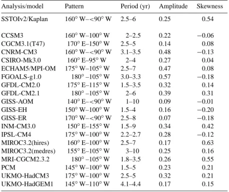
Table 2. Properties of the first EOF and associated time series (PC) of detrended monthly SST in the region 10◦S–10◦N, 120◦E–90◦W. The pattern denotes the longitudes of the contour of 80% of the peak value, the period denotes the height of the power spectrum at 50% of the peak value.

Analysis/model Pattern Period (yr) Amplitude Skewness SSTOIv2/Kaplan 160◦W–<90◦W 2.5–6 0.25 0.54 CCSM3 160◦W–100◦W 2–2.5 0.22 −0.06 CGCM3.1(T47) 170◦E–150◦W 2.5–5 0.14 0.08 CNRM-CM3 160◦W–<90◦W 3.1–3.5 0.48 −0.13 CSIRO-Mk3.0 160◦E–95◦W 2–4 0.27 0.04 ECHAM5/MPI-OM 175◦W–105◦W 2.5–7 0.47 0.08 FGOALS-g1.0 180◦–105◦W 3.0–3.3 0.57 −0.18 GFDL-CM2.0 175◦E–115◦W 1.5–3.5 0.32 0.14 GFDL-CM2.1 180◦–105◦W 2–6 0.39 0.31 GISS-AOM 140◦E–<90◦W 1–10 0.09 −0.01 GISS-EH 150◦W–100◦W 1.5–4 0.16 −0.20 GISS-ER 170◦W–<90◦W 2.5–8 0.07 −0.18 INM-CM3.0 150◦E–155◦W 1.5–9 0.34 0.42 IPSL-CM4 175◦W–100◦W 2.2–2.7 0.28 −0.12 MIROC3.2(hires) 160◦E–100◦W 2.5–7 0.17 0.63 MIROC3.2(medres) 155◦E–105◦W 3–10 0.25 0.16 MRI-CGCM2.3.2 180◦–105◦W 1.8–3.5 0.26 0.55 PCM 145◦W–100◦W 1.5–5 0.23 0.21 UKMO-HadCM3 175◦W–100◦W 2.5–5 0.32 0.21 UKMO-HadGEM1 145◦W–110◦W 4.1–4.4 0.17 0.15

The remaining models, ECHAM5/MPI-OM (Keenlyside et al., 2005), GFDL-CM2.1 (Wittenberg et al., 2005), MIROC3.2 (K-1 model developers, 2004) and HadCM3 (Collins, 2000b), (Figs 2d–f) resemble the observed ENSO reasonably well in SST variability. A noteworthy result is that the high-resolution version of MIROC3.2 has a much more realistic skewness than the medium resolution version.

4 Variability in wind stress and thermocline depth

While the variability of SST is a useful indicator of the gross characteristics of ENSO, the mechanisms which generate the coupled nature of the mode must be examined in order to fully evaluate model reliability. Hence we examine the vari-ables displayed in Fig. 1 by computing the standard deviation of the grid box SST variability at the maximum of the first SST EOF, the standard deviation of zonal wind stress at the maximum of the zonal wind response to this SST EOF, and the standard deviation of the depth of the 20◦_{C isotherm at} these two positions as a measure of the depth of the thermo-cline. Numerical values are shown in Table 3 with uncertain-ties quantified by the 95% confidence interval obtained using a bootstrapping approach with 7-month moving blocks. For the observations we use single buoys from the TAO array which we note are only available from the rather active last 20 years. Both factors lead to higher observed variability,

es-pecially in wind stress and SST, than can be expected from a long model simulation.

In many models thermocline variability is underestimated in comparison with the observations although we should note the caveat above regarding the length and period of the ob-served record. The wind stress variability depends strongly on the weather noise, so that the low variability in many models can be due either to a too weak ENSO signal or too little internal atmospheric variability (many models fail to simulate intraseasonal variability for example). Excep-tions are CNRM-CM3 and FGOALS-g1.0, which overesti-mate the SST variability, and HadCM3 and ECHAM5/MPI-OM, which seem well-balanced.

There are various instances in which a reasonable SST variability is generated from zonal wind stress and thermo-cline variability that is much lower than observed. These sensitivities will be explored in more detail in Sect. 6.

5 Wind response to SST perturbations

The amplitude of zonal wind stress variability in Table 3 is a combination of the slow variations that are part of the ENSO cycle and high-frequency weather noise integrated to the monthly time scale. To separate these contributions, the response of the atmosphere model to SST variations along the equator is examined. This may be done by regressing

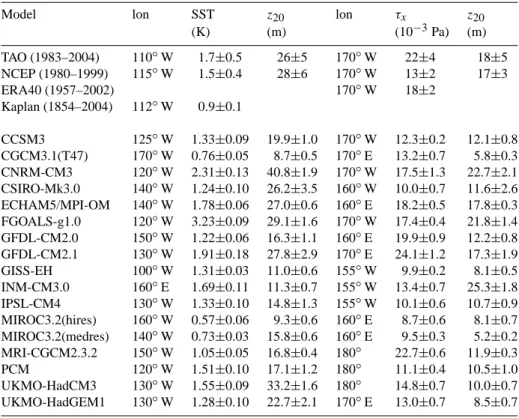
Table 3. The amplitude (standard deviation) of monthly SST and thermocline variability at the maximum of the first SST EOF, and amplitude

of zonal wind stress and thermocline variability (approximated by the depth of the 20◦C isotherm) at the point of maximum wind response. The errors denote the 95% confidence interval.

Model lon SST z20 lon τx z20

(K) (m) (10−3Pa) (m) TAO (1983–2004) 110◦W 1.7±0.5 26±5 170◦W 22±4 18±5 NCEP (1980–1999) 115◦W 1.5±0.4 28±6 170◦W 13±2 17±3 ERA40 (1957–2002) 170◦W 18±2 Kaplan (1854–2004) 112◦W 0.9±0.1 CCSM3 125◦W 1.33±0.09 19.9±1.0 170◦W 12.3±0.2 12.1±0.8 CGCM3.1(T47) 170◦W 0.76±0.05 8.7±0.5 170◦E 13.2±0.7 5.8±0.3 CNRM-CM3 120◦W 2.31±0.13 40.8±1.9 170◦W 17.5±1.3 22.7±2.1 CSIRO-Mk3.0 140◦W 1.24±0.10 26.2±3.5 160◦W 10.0±0.7 11.6±2.6 ECHAM5/MPI-OM 140◦W 1.78±0.06 27.0±0.6 160◦E 18.2±0.5 17.8±0.3 FGOALS-g1.0 120◦W 3.23±0.09 29.1±1.6 170◦W 17.4±0.4 21.8±1.4 GFDL-CM2.0 150◦W 1.22±0.06 16.3±1.1 160◦E 19.9±0.9 12.2±0.8 GFDL-CM2.1 130◦W 1.91±0.18 27.8±2.9 170◦E 24.1±1.2 17.3±1.9 GISS-EH 100◦W 1.31±0.03 11.0±0.6 155◦W 9.9±0.2 8.1±0.5 INM-CM3.0 160◦E 1.69±0.11 11.3±0.7 155◦W 13.4±0.7 25.3±1.8 IPSL-CM4 130◦W 1.33±0.10 14.8±1.3 155◦W 10.1±0.6 10.7±0.9 MIROC3.2(hires) 160◦W 0.57±0.06 9.3±0.6 160◦E 8.7±0.6 8.1±0.7 MIROC3.2(medres) 140◦W 0.73±0.03 15.8±0.6 160◦E 9.5±0.3 5.2±0.2 MRI-CGCM2.3.2 150◦W 1.05±0.05 16.8±0.4 180◦ 22.7±0.6 11.9±0.3 PCM 120◦W 1.51±0.10 17.1±1.2 180◦ 11.1±0.4 10.5±1.0 UKMO-HadCM3 130◦W 1.55±0.09 33.2±1.6 180◦ 14.8±0.7 10.0±0.7 UKMO-HadGEM1 130◦W 1.28±0.10 22.7±2.1 170◦E 13.0±0.7 8.5±0.7

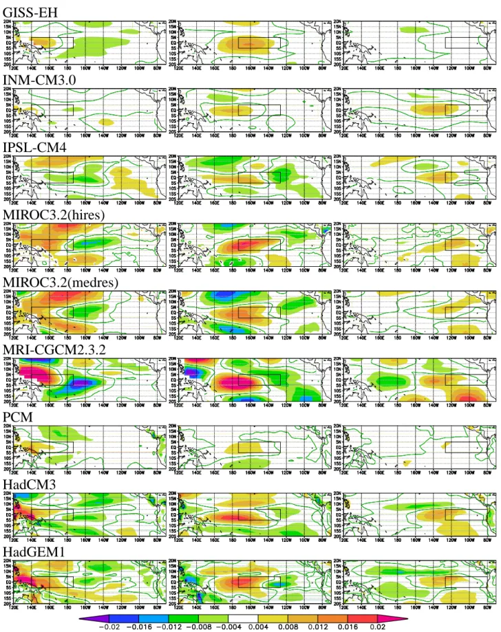
the zonal wind stress onto the first EOF of SST computed in Sect. 3, however the length of the simulations allows for a more detailed treatment. For each model we construct a statistical atmosphere model with as basis n equal-sized boxes along the equator in 5◦_S–5◦_{N, 140}◦_E–80◦_{W (e.g.} Von Storch and Zwiers, 2001, §8.3). The patterns show the average atmospheric response to an SST anomaly in this box only. For comparison with observations we only show re-sults for n=3 boxes. More detailed plots with n up to eight (for long runs with multiple ensemble members) confirm the findings.

The response to each box should to first order be a Gill-type pattern (Gill, 1980): westerly wind response to the east of the SST anomaly, weaker easterly response to the west, and possibly to the north and south of the SST anomaly. The strength of the response should depend on the background temperature: due to the nonlinear nature of convection the wind response is stronger over warm water than over colder water (e.g. Burgers and van Oldenborgh, 2003). The zero-line of the wind response is to the east of the heating anomaly (Clarke, 1994), which in turn is usually located to the west of the SST anomaly due to the temperature gradient and back-ground wind.

The ERA-40 data have been analyzed with three boxes (Figs. 3): western Pacific (warm pool), central Pacific

(ap-proximately equal to Ni˜no4) and eastern Pacific (cold tongue, similar to Ni˜no3). We see that the response to a temperature anomaly in the central box is indeed stronger than the re-sponse to an anomaly in the eastern box. In both of these regions the longitudinal offsets cancel: the zero wind stress anomaly line is near the middle of the SST anomaly. The response to the western box is “drowned” in the noise with only 45 years of data and only small SST variability.

The atmospheres of the climate models are less noisy as there is more data to construct the statistical atmosphere model. The responses are very diverse (Figs. 3 and 4). Almost all models show a weaker positive atmospheric re-sponse than the reanalysis when SST anomalies are present in the central or eastern Pacific. Only the MRI-CGCM2.3.2 model has a stronger response, with peak values twice those found in ERA-40. The CCSM3, CGCM3.1(T47), MIROC3.2(hires), HadCM3 and HadGEM1 models have a peak response that is only slightly weaker than the reanalysis, whereas the PCM model hardly shows any response at all. The weak response in most models explains why thermocline variability is in general lower than observed, although the exceptions (CNRM-CM3, FGOALS-g1.0, and INMCM3.0) show that there are other factors as well. A weak wind re-sponse will also suppress the non-linear aspects of ENSO in the ocean.

ERA40

CCSM3

CGCM3.1(T47)

CNRM-CM3

CSIRO-Mk3.0

ECHAM5/MPI-OM

FGOALS-g1.0

GFDL-CM2.0

GFDL-CM2.1

GISS-EH

INM-CM3.0

IPSL-CM4

MIROC3.2(hires)

MIROC3.2(medres)

MRI-CGCM2.3.2

PCM

HadCM3

HadGEM1

(a)

(b) (c)

(d) (e)

(f) (g)

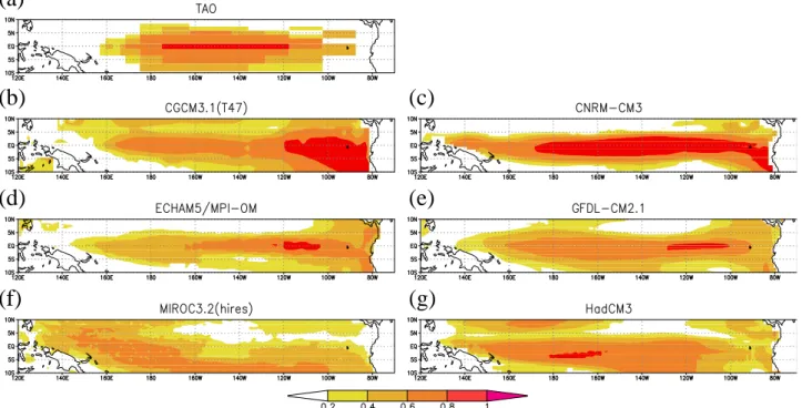
Fig. 5. Fraction of SST variance explained by the simple SST model Eq. (1) over an AR1 model (α=β=0) in (a) TAO data, (b)

CGCM3.1(T47), (c) CNRM-CM3, (d) ECHAM5/MPI-OM, (e) GFDL-CM2.1 (f) MIROC3.2(hires) and (g) HadCM3.

The equatorial negative response to the east of the SST anomaly in the central Pacific is also (much) weaker than ob-served in most models. Only the CCSM3, GFDL-CM2.0, GFDL-CM2.1 and HadGEM1 models have the same magni-tude. The off-equatorial response is important in setting the time scale of the ENSO cycle. The negative patterns of the Rossby wave response in the Gill pattern are hardly visible in the reanalysis, but much stronger in many models, especially CNRM-CM3 and MIROC3.2(medres). This is partly due to the much narrower latitudinal response in the models, a well-known problem with low resolution atmospheres (Guilyardi et al., 2004; Zelle et al., 2005), although not necessarily im-proved at higher resolutions. The narrower response in gen-eral leads to a shorter and more stable ENSO cycle. The northern off-equatorial response is positive rather than nega-tive in the FGOALS-g1.0, HadCM3 and HadGEM1 models. The location of the response is more easterly than in ob-servations in most models. Only in ECHAM5/MPI-OM, the GFDL models, IPSL-CM4 and MRI-CGCM2.3.2 the offset is zero, as observed. FGOALS-g1.0 shows a westerly offset. In most models the response is stronger over warmer water, as expected. Only in CCSM3 the strength is largest over the cold tongue (which in this model is in the central Pacific).

The response to SST anomalies in the western Pacific is stronger than in the reanalysis in most models. However, this is likely a problem in the reanalysis rather than the climate models, as SST variability is small in the warm pool, which means the response cannot be determined well by this tech-nique.

6 SST response to wind and thermocline perturbations

Most models have a wind response to wind anomalies that is too weak, and hence less thermocline variability than ob-served. There are three ways to obtain SST variability with a realistic amplitude from a weak wind response. Either SST responds more strongly to thermocline variability in the cold tongue, or SST responds more strongly to local wind anomalies on the edge of the warm pool, or SST damping is reduced. These processes have been separated by fitting the simple local SST equation (Burgers and van Oldenborgh, 2003)

dT

dt (x, y, t ) = α(x, y) z20(x, y, t − δ) + β(x, y) τx(x, y, t ) −γ (x, y) T (x, y, t ) (1) to both observations and GCM output. T is the local SST, upwelling and mixing of thermocline temperature anomalies are parametrized by α (nonlinear terms in this process are very small in TAO data). The finite upwelling time δ is pre-scribed from observations (Zelle et al., 2004) and varies from less than one month east of 130◦W to 5 months at the date line; this also agrees well with lag correlations of most model data. When it did not, no lag (δ=0) was used. The param-eter β describes the effects of zonal advection, upwelling, evaporation and variations in mixed-layer depth on SST, ne-glecting nonlinear terms. The damping parameter γ includes cloud feedback in the western Pacific.

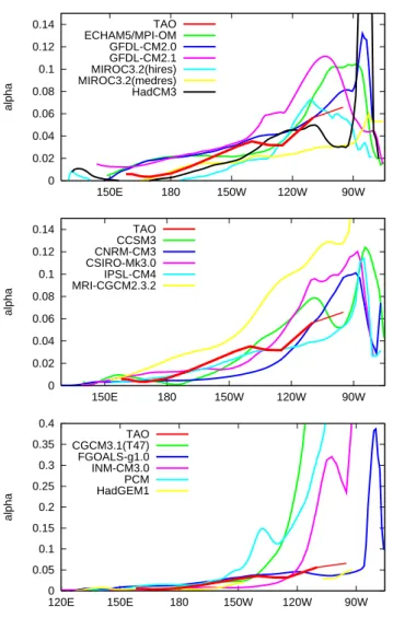
0 0.02 0.04 0.06 0.08 0.1 0.12 0.14 90W 120W 150W 180 150E alpha TAO ECHAM5/MPI-OM GFDL-CM2.0 GFDL-CM2.1 MIROC3.2(hires) MIROC3.2(medres) HadCM3 0 0.02 0.04 0.06 0.08 0.1 0.12 0.14 90W 120W 150W 180 150E alpha TAO CCSM3 CNRM-CM3 CSIRO-Mk3.0 IPSL-CM4 MRI-CGCM2.3.2 0 0.05 0.1 0.15 0.2 0.25 0.3 0.35 0.4 90W 120W 150W 180 150E 120E alpha TAO CGCM3.1(T47) FGOALS-g1.0 INM-CM3.0 PCM HadGEM1

Fig. 6. The parameter α (km−1month−1) that describes the effect of

thermocline anomalies on SST in Eq. (1) averaged over 3◦S–3◦N in the TAO observations and the climate models. Note the change of scale in the third panel.

In the TAO data the SST model Eq. (1) explains 60–80% of the variance along the equator (Fig. 5a), from 170◦_{E where} surface processes dominate to 110◦_{W in the cold tongue} where upwelling variability determines SST. The TAO buoy at EQ, 95◦W has only 80 months of observations, so the un-certainties in the fit parameters are quite large. In the climate models (examples are shown in Figs. 1b–f) the fraction of explained variance is similar in most models: higher when there is little weather noise (CNRM-CM3, FGOALS-g1.0), and usually lower in models with a weak ENSO (GISS-EH, MIROC3.2(hires)). In general the SST model fits the data reasonably well in the region where ENSO is active.

In Figs. 6, 7 and 8 the values of the parameters α, β and

γ−1are plotted as a function of longitude, averaged over the equatorial wave guide 3◦S–3◦N. In the GISS-EH model the parameters fluctuated so wildly that they have not been plot-ted. The other models are shown in three groups. The first

-50 0 50 100 150 200 90W 120W 150W 180 150E beta TAO ECHAM5/MPI-OM GFDL-CM2.0 GFDL-CM2.1 MIROC3.2(hires) MIROC3.2(medres) HadCM3 -50 0 50 100 150 200 90W 120W 150W 180 150E beta TAO CCSM3 CNRM-CM3 CSIRO-Mk3.0 IPSL-CM4 MRI-CGCM2.3.2 -100 0 100 200 300 400 90W 120W 150W 180 150E 120E beta TAO CGCM3.1(T47) FGOALS-g1.0 INM-CM3.0 PCM HadGEM1

Fig. 7. The parameter β (KPa−1month−1) that describes the effect

of wind stress anomalies on SST in Eq. (1) averaged over 3◦S–3◦N in the TAO observations and the climate models. Note the change of scale in the third panel.

one has wind stress sensitivities in the central Pacific β that are within 50% of those obtained from the TAO data, the sec-ond group is within a factor two and the third one outside of that.

We see that in most models, the weak zonal wind response found in Sect. 5 is compensated by an enhanced sensitiv-ity of SST to zonal wind stress β and a longer damping time γ−1_{, whereas the sensitivity to thermocline depth} varia-tions α clusters around the value deduced from observavaria-tions. A notable exception to this pattern is the MRI-CGCM2.3.2 model, in which the thermocline sensitivity is a factor three stronger than observed. In this model the damping term is stronger than in most other models (and close to the value fitted from observations) to keep the ENSO amplitude rea-sonable.

The models with a very regular ENSO cycle (CNRM-CM3, FGOALS-g1.0 and IPSL-CM4) all have weak

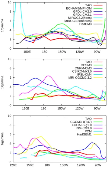
0 2 4 6 8 10 90W 120W 150W 180 150E 1/gamma TAO ECHAM5/MPI-OM GFDL-CM2.0 GFDL-CM2.1 MIROC3.2(hires) MIROC3.2(medres) HadCM3 0 2 4 6 8 10 90W 120W 150W 180 150E 1/gamma TAO CCSM3 CNRM-CM3 CSIRO-Mk3.0 IPSL-CM4 MRI-CGCM2.3.2 0 2 4 6 8 10 90W 120W 150W 180 150E 120E 1/gamma TAO CGCM3.1(T47) FGOALS-g1.0 INM-CM3.0 PCM HadGEM1

Fig. 8. The damping time γ−1(months) in Eq. (1), averaged over

3◦S–3◦N in the TAO observations and the climate models.

damping and strong wind feedback. Most models with a short ENSO cycle (CCSM, CSIRO-Mk3.0, CGCM3.1(T47), INM-CM3 and PCM) have too strong wind sensitivities in the central Pacific to compensate for the weak wind response. As the thermocline feedback is not enhanced, this implies that ENSO in these models is much more surface-driven than in the observations. SST in the HadGEM1 and GISS-EH models is not described well by Eq. (1).

The models with spectra that most resemble observations (ECHAM5/MPI-OM, GFDL-CM2.1, HadCM3, MIROC3.2 and to a lesser extent GFDL-CM2.0) show SST sensitivi-ties comparable to observations in the relevant regions: wind stress in the central Pacific, thermocline in the eastern Pa-cific.

7 ENSO in a warmer climate

After assessing the representation of ENSO in the current climate we next turn to the projections for the next

cen-tury. Specifically, projected changes in the mean state, am-plitude and skewness are considered. The SST expression of the ENSO cycle is not the most convenient index as it is mixed with the global warming signal itself. Instead, we use a pressure index comparable to the Southern Oscillation In-dex (Walker and Bliss, 1932; Berlage, 1957): the time series of the first EOF of SLP normalized to standard deviation over the area 30◦S–30◦N, 30◦E–60◦W. In order to minimize the influence of weather noise a 5-month running mean is applied. In the ERA-40 reanalysis this index is strongly cor-related with the traditional Darwin-Tahiti SOI (r=−0.91). For scenario experiments the pattern obtained in the current climate is projected onto the SLP field of the future (in the IPSL and MIROC3.2(hires) models, the second EOF corre-sponds to the Southern Oscillation). The patterns are in gen-eral very realistic (Fig. 9) and do not change significantly under global warming.

For ENSO variability and skewness the first EOF of SST in the region 10◦S–10◦N, 120◦E–90◦W with a 10 yr run-ning mean subtracted was also considered. The results were identical to the ones obtained with the SLP index.

In Table 4 the results are shown as the difference in the mean value of the indices in the future climate divided by the standard deviation of the current climate, the ratio of the standard deviations, and the skewness. The future climate is represented by the last 50 years of the scenario run (SRES A2, SRES a1B or 1%/year compounded CO2increase). Un-certainty estimates (95% limits) have been computed with a moving block bootstrap procedure. The subjective confi-dence level attached to the prediction (medium, high) reflects whether ENSO in the model seems to be based on the same physical processes as in the observations, as determined in the previous sections.

As in previous studies (e.g. Collins and the CMIP Mod-elling Groups, 2005), changes in the mean state range from more La Ni˜na-like conditions to more El Ni˜no-like mean conditions. The low-resolution models CGCM3.0(T47), GISS-EH, INM-CM3, IPSL-CM4 and PCM project a change to more La Ni˜na-like mean conditions, but these all have been assigned a lower confidence level due to either a too regular cycle or too much of a surface-driven ENSO cy-cle. In most of these models this shift is due to a large change in the Indian Ocean or off-equatorial Pacific Ocean projecting onto the ENSO pattern. The only model in which the time change in surface pressure resembles the Southern Oscillation is INM-CM3.0, however, in the stabilisation pe-riod after 2100 this model switches to a more El-Ni˜no-like state.

CCSM3, CNRM-CM3, ECHAM5/MPI-OM, FGOALS-g1.0, the MIROC3.2 models and MRI-CGCM2.3.2 show a shift to on average more El Ni˜no-like mean conditions. Al-most all these shifts are about one quarter of the interannual standard deviation. (The much larger shift in the high reso-lution version of the MIROC3.2 model is due to a disconti-nuity between the twentieth century run and the SRES A1B

(a)

(b) (c)

(d) (e)

(f) (g)

Fig. 9. First EOF of normalized sea-level pressure over the region 30◦S–30◦N, 30◦E–60◦W (α=β=0) in (a) TAO data, (b) CGCM3.1(T47),

(c) CNRM-CM3, (d) ECHAM5/MPI-OM, (e) GFDL-CM2.1, (f) MIROC3.2(hires) (second EOF) and (g) HadCM3.

run; the scenario run indicates a much smaller shift in the mean state.) Again, only in ECHAM5/MPI-OM and MRI-CGCM2.3.2 the shift resembles the Southern Oscillation pat-tern.

The remaining models, CSIRO-Mk3.0, both GFDL mod-els and the Hadley Centre modmod-els HadCM3 and HadGEM1 show no significant change to a more El Ni˜no or La Ni˜na-like climatology.

The trends in sea-level pressure are not necessarily con-sistent with the trends in SST, as investigated by others1. Quite a few models show warming in the cold tongue, but no change in psl, or even a shift to La Ni˜na (CGCM3.1(T47), IPSL-CM4). This could be understood as a change 1T in the cold tongue having less effect on air pressure than the same change in the warm pool. As the main reason for this study is the effect of ENSO on the weather, we consider the pressure trends to be the more important ones.

1_{E.g., E. Guilyardi (2005) and W. J. Merryfield: Changes to}

ENSO under CO₂doubling in the IPCC AR4 coupled climate mod-els, J. Climate, submitted, 2005.

The range in forecasts for the variability is just as large. The CCSM3, CGCM3.0(T47), FGOALS-g1.0, MIROC3.2(medres) and PCM models have statis-tically significant less variability in the last 50 years of the scenario runs; the ECHAM5/MPI-OM, GFDL-CM2.0, MRI-CGCM2.3.2 and HadCM3 models show more activity and the other models (CNRM-CM3, CSIRO-Mk3.0, GFDL-CM2.1, GISS-EH, INM-CM3, IPSL-CM4, MIROC3.2(hires) and HadGEM1) have no significant change in standard deviation under global warming. The difference between the two versions of the GFDL model (a factor 1.21±0.12 higher standard deviation in CM2.0 and 0.88±0.13 in CM2.1) shows that the change in variability is due to small details of the model, similar to that seen in Collins (2000a). Note that the changes are of the same order as those observed in the SOI over the periode 1866–2004, so that the predicted change in standard deviation is often only significant with more than one ensemble member, and hence unobservable in reality.

Table 4. The change in mean value normalized to the standard deviation, the ratio of the standard deviation and change in skewness of the

SLP pattern between the current climate and the last 50 years of a scenario experiment. Positive values denote El Ni˜no, negative La Ni˜na. The errors denote the 95% CL interval. The MIROC3.2(hires) 1 mean is unreliable due to a discontinuity.

Model Confidence Scenarios 1mean 1s.d. 1skewness CCSM3 20c3m sresa2 0.61±0.08 0.81±0.05 0.04±0.27 CGCM3.1(T47) 20c3m sresa2 -0.38±0.16 0.75±0.09 -0.06±0.31 CNRM-CM3 20c3m sresa2 0.46±0.22 1.09±0.11 -0.09±0.29 CSIRO-Mk3.0 20c3m sresa2 0.07±0.15 1.03±0.10 0.05±0.32 ECHAM5/MPI-OM high 20c3m sresa2 0.22±0.12 1.14±0.08 -0.15±0.20 FGOALS-g1.0 20c3m sresa1b 0.12±0.09 0.64±0.04 -0.18±0.14 GFDL-CM2.0 high 20c3m sresa2 0.02±0.23 1.21±0.12 0.12±0.29 GFDL-CM2.1 high 20c3m sresa2 -0.10±0.16 0.88±0.13 -0.03±0.46 GISS-EH 20c3m 1pctto2x -0.34±0.12 1.00±0.09 -0.03±0.35 INM-CM3.0 20c3m sresa2 -0.76±0.19 0.92±0.15 0.42±0.49 IPSL-CM4 20c3m sresa2 -0.45±0.20 1.10±0.12 -0.07±0.29 MIROC3.2(hires) medium 20c3m sresa1b (1.13±0.20)? 0.97±0.17 -0.29±0.58 MIROC3.2(medres) medium 20c3m sresa2 0.25±0.10 0.86±0.07 0.12±0.27 MRI-CGCM2.3.2 20c3m sresa2 0.25±0.11 1.26±0.07 -0.23±0.16 PCM 20c3m sresa2 -0.12±0.11 0.89±0.07 0.08±0.29 UKMO-HadCM3 high 20c3m sresa2 0.00±0.20 1.16±0.13 0.07±0.35 UKMO-HadGEM1 picntrl 1pctto2x 0.01±0.23 1.10±0.13 -0.15±0.34

Due to the limited number of years (50) in the future pe-riod, only the FGOALS-g1.0 and MRI-CGCM2.3.2 models show a shift in skewness that is statistically significantly dif-ferent from zero. However, even the models that resemble reality most do not reproduce the observed skewness of SST, thermocline depth and zonal wind stress very well, so they are unlikely to contain correctly the nonlinear mechanisms that determine the differences between El Ni˜no and La Ni˜na. We therefore do not attach much significance to the fact that these models do not show much change in skewness.

8 Conclusions

We have studied ENSO-like oscillations in the equatorial Pa-cific in the 19 climate models that had made data available in the PCMDI archive at the time of submission. First, the simi-larity of these oscillations with the observed ENSO cycle has been determined. Two models (GISS-AOM and GISS-ER) do not show ENSO-like variability and are excluded from the analysis.

Three models (CNRM-CM3, FGOALS-g1.0 and IPSL-CM4) show very regular oscillations with negative skewness, in contrast to the real irregular ENSO cycle with positive skewness. These models seem to operate in a different dy-namical regime than the point close to stability that the ob-served ENSO is thought to occupy. Another group of models (CCSM3, CGCM3.1(T47)), has a more westerly ENSO pat-tern than observed, a shorter period, a lower amplitude and no skewness. Other models (CSIRO-Mk3.0, GFDL-CM2.0, GISS-EH, INM-CM3, MRI-CGCM2.3.2, PCM) share most of these properties, which often occur in coarse-resolution

models. ECHAM5/MPI-OM, GFDL-CM2.1, MIROC3.2 and HadCM3 display the most realistic time series proper-ties. HadGEM1 is unlike other models with a fairly narrow spectral peak but positive skewness.

The reasons for these diverse modeled ENSO cycles be-come clearer when considering the strength of the zonal wind response to equatorial SST anomalies and the SST response to wind and thermocline depth anomalies. Most models show a zonal wind response that is weaker and more confined in latitude than the observations. This is compensated by a stronger direct SST response to wind anomalies and weaker damping of surface temperature than the observations indi-cate, whereas the reaction to thermocline depth anomalies is similar to estimates from TAO data. In these models ENSO is therefore more surface-driven than thermocline-driven. A different mixture occurs in the MRI model, in which SST reacts very strongly to both wind and thermocline depth anomalies, and is more damped to obtain a realistic SST variability. The ECHAM5/MPI-OM, CM2.0, GFDL-CM2.1, MIROC3.2 and HadCM3 models show a fairly real-istic balance between the two feedback loops of the ENSO cycle and the forecasts from these models are considered most reliable.

In these models the forecasts for the mean state of ENSO in 2051–2100 in an SRES A2 scenario range from no change (four models) to a small shift (25% of the standard devi-ation) towards more El Ni˜no-like conditions (two models) in surface pressure. The variability projections vary from a slight increase, by 15% (three models), through no change (two models) to a decreases by 15% (one model). The pos-sible changes are of the same size as the observed decadal

variability over the last century and only statistically signif-icant for multiple ensemble members. It will therefore be difficult to verify with only one realization of reality. The statistical and systematic errors in skewness are too large to say anything with any degree of certainty about the relative strength of El Ni˜no and La Ni˜na events in a future climate.

This is only a first assessment of the characteristics of ENSO variability in climate models, covering what we judge to be the most important aspects. In the conceptual model of the ENSO cycle of Fig. 1 we have not considered the char-acteristics of the external noise, nor the relationship between zonal wind stress anomalies and thermocline perturbations. The seasonal cycle has been neglected throughout. Outside of this simplified picture the radiation and latent heat contri-butions to SST variability should be studied in more detail. The causes of changes in ENSO properties in the modeled future climate have also not been investigated in this study but should be a priority for future work.

Acknowledgements. We acknowledge the international modeling

groups for providing their data for analysis, the Program for Cli-mate Model Diagnosis and Intercomparison (PCMDI) for collect-ing and archivcollect-ing the model data, the JSC/CLIVAR Workcollect-ing Group on Coupled Modelling (WGCM) and their Coupled Model Inter-comparison Project (CMIP) and Climate Simulation Panel for or-ganizing the model data analysis activity, and the IPCC WG1 TSU for technical support. The IPCC Data Archive at Lawrence Liver-more National Laboratory is supported by the Office of Science, US Department of Energy. MC was supported by the UK De-partment of the Environment, Food and Rural Affairs under Con-tract PECD/7/12/37 and by the EU ENSEMBLES and DYNAMITE projects.

This research is supported by the Research Council for Earth and Life Sciences (ALW) of the Netherlands Organisation for Scientific Research (NWO).

Edited by: D. Stevens

References

Behringer, D. W., Ji, M., and Leetmaa, A.: An Improved coupled model for ENSO prediction and implications for ocean initializa-tion, Part I: The ocean data assimilation system, Mon. Wea. Rev., 126, 1013–1021, 1998.

Berlage, H. P.: Fluctuations of the general atmospheric circulation of more than one year, their nature and prognostic value, no. 69 in Mededelingen en verhandelingen, KNMI, De Bilt, Netherlands, 1957.

Bjerknes, J.: A possible response of the atmospheric Hadley circu-lation to equatorial anomalies of ocean temperature, Tellus, 18, 820–829, 1966.

Burgers, G. and van Oldenborgh, G. J.: On the Impact of Local Feedbacks in the Central Pacific on the ENSO cycle, J. Climate, 16, 2396–2407, 2003.

Cai, W., Collier, M. A., Gordon, H. B., and Waterman, L. J.: Strong ENSO variability and a super-ENSO pair in the CSIRO coupled climate model, Mon. Wea. Rev., 131, 1189–1210, 2003.

Clarke, A. J.: Why Are Surface Equatorial ENSO Winds Anoma-lously Westerly under Anomalous Large-Scale Convection?, J. Climate, 7, 1623–1627, 1994.

Codron, F., Vintzileos, A., and R., S.: Influence of Mean State Changes on the Structure of ENSO in a Tropical Coupled GCM, J. Climate, 14, 730–742, 2001.

Collins, M.: Uncertainties in the response of ENSO to Greenhouse Warming, Geophys. Res. Lett., 27, 3509–3513, 2000a.

Collins, M.: The El-Ni˜no Southern Oscillation in the second Hadley Centre coupled model and its response to greenhouse warming, J. Climate, 13, 1299–1312, 2000b.

Collins, M. and the CMIP Modelling Groups: El Ni˜no- or La Ni˜na-like climate change?, Climate Dyn., 24, 89–104, 2005.

Collins, W. D., Bitz, C. M., Blackmon, M. I., Bonan, G. B., Brether-ton, C. S., CarBrether-ton, J. A., Chang, P., Doney, S. C., Hack, J. J., Henderson, T. B., Kiehl, J. T., Large, W. G., McKenna, D. S., Santer, B. D., and Smith, R. D.: The Community Climate Sys-tem Model: CCSM3, J. Climate, accepted, 2005.

Delworth, T. L., Broccoli, A. J., Rosati, A., Stouffer, R. J., Balaji, V., Beesley, J. A., Cooke,W. F., Dixon, K.W., Dunne, J., Dunne, K. A., Durachta, J. W., Findell, K. L., Ginoux, P., Gnanadesikan, A., Gordon, C. T., Griffies, S. M., Gudgel, R., Harrison, M. J., Held, I. M., Hemler, R. S., Horowitz, L. W., Klein, S. A., Knut-son, T. R., Kushner, P. J., Langenhorst, A. R., Lee, H. C., Lin1, S. J., Lu, J., Malyshev, S. L., Milly, P. C. D., Ramaswamy, V., Rus-sell, J., Schwarzkopf, M. D., Shevliakova, E., Sirutis, J. J., Spel-man, M. J., Stern, W. F., Winton, M., Wittenberg, A. T., WySpel-man, B., Zeng, F., and Zhang, R.: GFDLs CM2 global coupled climate models – Part 1: Formulation and simulation characteristics, J. Climate, in press, 2005.

Dijkstra, H. A.: Nonlinear Physical Oceanography, Kluwer Aca-demic Publishers, Dordrecht, The Netherlands, 2000.

Fedorov, A. V. and Philander, S. G.: A stability analysis of trop-ical ocean-atmophere interactions: bridging measurements and theory for El Ni˜no, J. Climate, 14, 3086–3101, 2001.

Gill, A. E.: Some simple solutions for heat induced tropical circu-lation, Quart. J. Roy. Meteor. Soc., 106, 447–462, 1980. Gordon, C., Cooper, C., Senior, C. A., Banks, H., Gregory, J. M.,

Johns, T. C., Mitchell, J. F. B., and Wood, R. A.: The Simulation of SST, sea ice extents and ocean heat transport in a version of the Hadley Centre coupled model without flux adjustments, Climate Dyn., 16, 147–168, 2000.

Gordon, H. B., Rotstayn, L. D., McGregor, J. L., Dix, M. R., Kowal-czyk, E. A., O’Farrell, S. P., Waterman, L. J., Hirst, A. C., Wil-son, S. G., Collier, M. A., WatterWil-son, I. G., and Elliott, T. I.: The CSIRO Mk3 Climate System Model, Tech. Rep. 60, CSIRO Atmospheric Research, Aspendale, 2002.

Guilyardi, E., Gualdi, S., Slingo, J., Navarro, A., Delecluse, P., Cole, J., Madec, G., Roberts, M., Latif, M., and Terray, L.: Rep-resenting El Ni˜no in coupled ocean-atmosphere GCMs: the dom-inant role of the atmosphere component, J. Climate, 17, 4623– 4629, 2004.

Guilyardi, E.: El Ni˜no – mean state – seasonal cycle interactions in a multi-model ensemble, Climate Dyn., accepted, 2005. Johns, T. et al.: HadGEM1 – Model description and analysis of

pre-liminary experiments for the IPCC Fourth Assessment Report, Tech. Rep. 55, UK Met Office, Exeter, UK, 2004.

Jungclaus, J., Botzet, M., Haak, H., Keenlyside, N., Luo, J.-J., Latif, M., Marotzke, J., Mikolajewicz, U., and Roeckner, E.: Ocean

cir-culation and tropical variability in the AOGCM ECHAM5 /MPI-OM, J. Climate, accepted, 2005.

K-1 model developers: K-1 coupled model (MIROC) description, Tech. Rep. 1, Center for Climate System Research, University of Tokyo, 2004.

Kaplan, A., Cane, M. A., Kushnir, Y., Clement, A. C., Blumen-thal, M. B., and Rajagopalan, B.: Analyses of global sea surface temperature 1856–1991, J. Geophys. Res., 103, 18 567–18 589, 1998.

Keenlyside, N., Latif, M., Botzet, M., Jungclaus, J., and Schulzweida, U.: A coupled method for initializing El Ni˜no Southern Oscillation forecasts using sea surface temperature, Tellus, A57, 340, 2005.

Kim, S.-J., Flato, G. M., de Boer, G. J., and McFarlane, N. A.: A coupled climate model simulation of the Last Glacial Maximum, Part 1: transient multi-decadal response, Climate Dyn., 19, 515– 537, 2002.

Knutson, T. R., Manabe, S., and Gu, D.: Simulated ENSO in a global coupled ocean-atmosphere model: Multidecadal ampli-tude modulation and CO2 sensitivity., J. Climate, 10, 42–63,

1997.

Lucarini, L. and Russell, G. L.: Comparison of mean climate trends in the northern hemisphere between National Centers for Envi-ronmental Prediction and two atmosphere-ocean model forced runs, J. Geophys. Res., D15, 2002.

Marti, O. et al.: The new IPSL climate system model: IPSL-CM4, Tech. rep., Institut Pierre Simon Laplace des Sciences de l’Environnement Global, IPSL, Case 101, 4 place Jussieu, Paris, France, 2005.

McPhaden, M. J., Busalacchi, A. J., Cheney, R., Donguy, J. R., Gage, K. S., Halpern, D., Ji, M., Julian, P., Meyers, G., Mitchum, G. T., Niiler, P. P., Picaut, J., Reynolds, R. W., Smith, N., and Takeuchi, K.: The Tropical Ocean Global Atmosphere (TOGA) observing system: a decade of progress, J. Geophys. Res., 103, 14 169–14 240, 1998.

Meehl, G. A., Branstator, G. W., and Washington, W. M.: Tropi-cal Pacific Interannual Variability and CO2Climate Change, J.

Climate, 6, 42–63, 1993.

Meehl, G. A., Gent, P. R., Arblaster, J. M., Otto-Bliesner, B. L., Brady, E. C., and Craig, A.: Factors that affect the amplitude of El Ni˜no in global coupled climate models, Climate Dyn., 17, 515–526, 2001.

Murphy, J. M., Sexton, D. M. H., Barnett, D. N., Jones, G. S., Webb, M. J., Collins, M., and Stainforth, D. A.: Quantification of mod-elling uncertainties in a large ensemble of climate change simu-lations, Nature, 430, 768–772, 2004.

Neelin, J. D., Battisti, D. S., Hirst, A. C., Jin, F.-F., Wakata, Y., Yamagata, T., and Zebiak, S.: ENSO theory, J. Geophys. Res., 103, 14 261–14 290, 1998.

Otto-Bliesner, B. and Brady, E.: Tropical Pacific variability in the NCAR Climate System Model, J. Climate, 14, 3587–3607, 2001. Picaut, J., Ioulalen, M., Menkes, C., Delcroix, T., and McPhaden, M. J.: Mechanism of the Zonal Displacement of the Pacific warm pool: implications for ENSO, Science, 274, 1486–1489, 1996. Reynolds, R. W., Rayner, N. A., Smith, T. M., Stokes, D. C., and

Wang, W.: An Improved In Situ and Satellite SST Analysis for Climate, J. Climate, 15, 1609–1625, 2002.

Schmidt, G. A. et al.: Present day atmospheric simulations using GISS ModelE: Comparison to in-situ, satellite and reanalysis

data, J. Climate, accepted, 2005.

Tett, S.: Simulation of El-Ni˜no/Southern Oscillation like variability in a global AOGCM and its response to CO₂increase, J. Climate, 8, 1473–1502, 1995.

Timmermann, A., Oberhuber, J., Bacher, A., Esch, M., Latif, M., and Roeckner, E.: Increased El-Ni˜no frequency in a climate model forced by future greenhouse warming, Nature, 398, 694– 696, 1999.

Uppala, S. M., K˚alberg, P. W., Simmons, A. J., Andrae, U., da Costa Bechtold, V., Fiorino, M., Gibson, J. K., Haseler, J., Hernandez, A., Kelly, G., Li, X., Onogi, K., Saarinen, S., Sokka, N., Allan, R. P., Anderson, E., Arpe, K., Balmaseda, M. A., Bel-jaars, A. C. M., van den Berg, L., Bidlot, J., Borman, N., Caires, S., Dethof, A., Dragosavac, M., Fisher, M., Fuentes, M., Hage-mann, S., H´olm, E., Hoskins, B. J., Isaksen, L., Janssen, P. A. E. M., Jenne, R., McNally, A., Mahfouf, J.-F., Mocrette, J.-J., Rayner, N. A., Saunders, R. W., Simon, P., Sterl, A., Trenberth, K. E., Untch, A., Vasiljevic, D., Viterbo, P., and Woollen, J.: The ERA-40 re-analysis, Quart. J. Roy. Meteor. Soc., accepted, 2005. van der Vaart, P. C. F.: Nonlinear tropical climate dynamics, Ph.D.

thesis, Universiteit Utrecht, 1998.

Volodin, E. M. and Diansky, N. A.: El-Ni˜no reproduction in cou-pled general circulation model of atmosphere and ocean, Russian meteorology and hydrology, 12, 5–14, 2004.

Von Storch, H. and Zwiers, F. W.: Statistical Analysis in Climate Research, Cambridge University Press, Cambridge, UK, ISBN 0521012309, 2001.

Walker, G. T. and Bliss, E. W.: World Weather V, Mem. Roy. Me-teor. Soc., 4, 53–84, 1932.

Washington, W. M., Weatherly, J. W., Meehl, G. A., Semtner Jr., A. J., Bettge, T. W., Craig, A. P., Strand Jr., W. G., Arblaster, J., Wayland, V. B., James, R., and Zhang, Y.: Parallel climate model (PCM) control and transient simulations, Climate Dyn., 16, 755–774, 2000.

Wittenberg, A., Rosati, A., Lau, N.-C., and Ploshay, J.: GFDL’s CM2 global coupled climate models, Part 3: Tropical Pacific Cli-mate and ENSO, J. CliCli-mate, in press, 2005.

Wyrtki, K.: El Ni˜no – The dynamic response of the equatorial Pa-cific Ocean to atmospheric forcing, J. Phys. Oceanogr., 5, 572– 584, 1975.

Yu, B. and Boer, G.: The roles of radiation and dynamical processes in the El Ni˜no-like response to global warming, Climate Dyn., 19, 539–554, 2002.

Yu, Y., Zhang, X., and Guo, Y.: Global coupled ocean- atmosphere general circulation models in LASG/IAP, Adv. Atmos. Sci., 21, 444–455, 2004.

Yukimoto, S. and Noda, A.: Improvements of the Meteorologi-cal Research Institute Global Ocean-atmosphere Coupled GCM (MRI-CGCM2) and its climate sensitivity, Tech. Rep. 10, NIES, Japan, 2002.

Zelle, H., Appeldoorn, G., Burgers, G., and van Oldenborgh, G. J.: On the relationship between sea surface temperature and thermo-cline depth in the eastern equatorial Pacific, J. Phys. Oceanogr., 34, 643–655, 2004.

Zelle, H., van Oldenborgh, G. J., Burgers, G., and Dijkstra, H. A.: El Ni˜no and Global Change: Results from Ensemble Simulations with the NCAR CCSM, J. Climate, in press, 2005.