HAL Id: hal-00296364
https://hal.archives-ouvertes.fr/hal-00296364
Submitted on 19 Oct 2007
HAL is a multi-disciplinary open access
archive for the deposit and dissemination of
sci-entific research documents, whether they are
pub-lished or not. The documents may come from
teaching and research institutions in France or
abroad, or from public or private research centers.
L’archive ouverte pluridisciplinaire HAL, est
destinée au dépôt et à la diffusion de documents
scientifiques de niveau recherche, publiés ou non,
émanant des établissements d’enseignement et de
recherche français ou étrangers, des laboratoires
publics ou privés.
condensation nuclei: processes and uncertainties
evaluated with a global aerosol microphysics model
J. R. Pierce, K. Chen, P. J. Adams
To cite this version:
J. R. Pierce, K. Chen, P. J. Adams. Contribution of primary carbonaceous aerosol to cloud
con-densation nuclei: processes and uncertainties evaluated with a global aerosol microphysics model.
Atmospheric Chemistry and Physics, European Geosciences Union, 2007, 7 (20), pp.5447-5466.
�hal-00296364�
www.atmos-chem-phys.net/7/5447/2007/ © Author(s) 2007. This work is licensed under a Creative Commons License.
Chemistry
and Physics
Contribution of primary carbonaceous aerosol to cloud
condensation nuclei: processes and uncertainties evaluated with a
global aerosol microphysics model
J. R. Pierce1, K. Chen2, and P. J. Adams2,3
1Department of Chemical Engineering, Carnegie Mellon University, Pittsburgh, PA, USA
2Department of Civil and Environmental Engineering, Carnegie Mellon University, Pittsburgh, PA, USA 3Department of Engineering and Public Policy, Carnegie Mellon University, Pittsburgh, PA, USA
Received: 10 April 2007 – Published in Atmos. Chem. Phys. Discuss.: 4 June 2007 Revised: 3 September 2007 – Accepted: 18 October 2007 – Published: 19 October 2007
Abstract. This paper explores the impacts of primary
car-bonaceous aerosol on cloud condensation nuclei (CCN) con-centrations in a global climate model with size-resolved aerosol microphysics. Organic matter (OM) and elemen-tal carbon (EC) from two emissions inventories were in-corporated into a preexisting model with sulfate and sea-salt aerosol. The addition of primary carbonaceous aerosol increased CCN(0.2%) concentrations by 65–90% in the globally averaged surface layer depending on the carbona-ceous emissions inventory used. Sensitivity studies were performed to determine the relative importance of organic solubility/hygroscopicity in predicting CCN. In a sensitiv-ity study where carbonaceous aerosol was assumed to be completely insoluble, concentrations of CCN(0.2%) still in-creased by 40–50% globally over the no carbonaceous simu-lation because primary carbonaceous emissions were able to become CCN via condensation of sulfuric acid. This shows that approximately half of the contribution of primary car-bonaceous particles to CCN in our model comes from the addition of new particles (seeding effect) and half from the contribution of organic solute (solute effect). The solute ef-fect tends to dominate more in areas where there is less in-organic aerosol than in-organic aerosol and the seeding effect tends to dominate in areas where there is more inorganic aerosol than organic aerosol. It was found that an accu-rate simulation of the number size distribution is necessary to predict the CCN concentration but assuming an average chemical composition will generally give a CCN concentra-tion within a factor of 2. If a “typical” size distribuconcentra-tion is assumed for each species when calculating CCN, such as is done in bulk aerosol models, the mean error relative to a simulation with size resolved microphysics is on the or-der of 35%. Predicted values of carbonaceous aerosol mass
Correspondence to: J. R. Pierce ([email protected])
and aerosol number were compared to observations and the model showed average errors of a factor of 3 for carbona-ceous mass and a factor of 4 for total aerosol number; how-ever, errors in the accumulation mode concentrations were found to be lower in comparisons with European and marine observations.. The errors in CN and carbonaceous mass may be reduced by improving the emission size distributions of both primary sulfate and primary carbonaceous aerosol.
1 Introduction
Radiative forcing by aerosols is an important contributor to climate change (Forster et al., 2007). Compared to the positive (warming) radiative forcing caused by greenhouse gases, the magnitude of the negative (cooling) radiative forc-ing by aerosols remains uncertain. The largest uncertainty in aerosol forcing of climate is the indirect effect, wherein an-thropogenic aerosols perturb the earth’s climate by increas-ing cloud reflectance (Albrecht, 1989; Twomey, 1974). This occurs when anthropogenic activities increase the number of aerosol particles that serve as nuclei upon which cloud droplets form (cloud condensation nuclei or CCN). The con-sequent increase in cloud droplet number concentrations (CDNC) leads to more reflective clouds that may have longer lifetimes (Albrecht, 1989; Twomey, 1974). The Intergovern-mental Panel on Climate Change (IPCC) has estimated that the globally and annually averaged indirect aerosol radiative forcing lies between −0.3 and −1.8 W m−2, with a median
value of −0.7 W m−2, as compared with +2.5 W m−2
im-posed by changes in greenhouse gases (Forster et al., 2007). This estimate includes only the effect of aerosols on cloud albedo, neglecting changes in cloud cover. Uncertainty in the magnitude of aerosol forcing has plagued efforts to quan-tify the sensitivity of climate to anthropogenic perturbations
(Andreae et al., 2005; Schwartz, 2004). Clearly it is neces-sary to improve our estimates of the indirect effect.
To estimate the indirect radiative forcing, it is essential to understand the activation of aerosol particles to form cloud droplets under supersaturated conditions. Whether or not a particle activates depends on the ambient supersaturation as well as particle size and composition. Therefore, a physically based model of the indirect effect should predict the number size distribution of aerosols and the chemical composition of each size range to predict the number of CCN for any super-saturation. Knowledge of aerosol mixing state is also essen-tial for correct prediction of CCN activation behavior.
Carbonaceous aerosols, mainly produced from fossil fuel and biomass combustion, are composed of two classes of ma-terial: elemental carbon (EC) and organic matter (OM). Ele-mental carbon is emitted directly from primary sources. OM, in contrast, is both emitted as particulates (primary OM) and also condensed in the atmosphere from semi-volatile oxida-tion products of volatile organic compounds. The latter is referred to as secondary organic aerosol (SOA).
Carbonaceous aerosols are considered to be a strong contributor to the indirect effect (Novakov and Penner, 1993). Lohmann et al. (2000) predict an indirect effect of −0.9 W m−2 from anthropogenic carbonaceous aerosol
alone compared to −0.4 W m−2 from sulfate aerosol alone,
and −1.1 W m−2 from an internal mixture of the two.
Chuang et al. (2002) estimate a total cloud albedo forc-ing of −1.85 W m−2, with −0.30 W m−2and −1.51 W m−2
from sulfate and carbonaceous aerosols alone, respectively. Hitzenberger et al. (1999) observed, in rural Europe sites, that carbonaceous material contributed up to 67% of total aerosol mass in CCN size range; in urban areas, the con-tribution of OM to the total mass concentration in this size range was 48%. Based on these studies, it seems likely that carbonaceous aerosol plays an important role in the tropo-spheric CCN budget. Therefore, it is essential to understand the global distribution of mass and number concentrations and size distribution of carbonaceous aerosols.
A number of previous modeling studies using bulk aerosol models have been performed to estimate the global distribu-tion of carbonaceous aerosols (Chung and Seinfeld, 2002; Cooke et al., 1999; Cooke and Wilson, 1996; Liousse et al., 1996; Lohmann et al., 2000; Penner et al., 1998; Reddy and Boucher, 2004). However, these studies must make assump-tions about the aerosol size distribution or use empirical re-lations to predict CDNC from their predicted aerosol mass. Besides the uncertainties inherent in the empirical approach, it has the disadvantage of concealing the physical processes that control CCN concentrations, introducing the difficulty of testing the sensitivity of model behavior to uncertainties or changes in specific microphysical processes such as nu-cleation.
The most fundamental, albeit computationally intensive, method predicting aerosol size distributions results is solv-ing aerosol microphysics explicitly ussolv-ing the aerosol
gen-eral dynamic equation (Seinfeld and Pandis, 1998), which governs how the aerosol size distribution evolves as a re-sult of the microphysical processes of nucleation, conden-sation, and coagulation. Numerical algorithms for treating aerosol microphysics can be broadly categorized as modal, based, or sectional. To our knowledge, moment-based approaches have not been implemented into global models for the purposes of predicting CCN concentrations although regional-scale applications have been demonstrated (Yu et al., 2003). Modal algorithms that represent the aerosol size distribution as the sum of several lognormal distribu-tions, each characterized by a number concentration, median diameter, and geometric standard deviation, have been devel-oped by Herzog et al. (2004), Jung et al. (2004) and Vignati et al. (2004) and implemented in Easter et al. (2004), Ghan et al. (2001), Stier et al. (2005) and Wilson et al. (2001) in global models. Except for Jung et al. (2004), the versions of the modal approach cited here have prescribed constant val-ues to the geometric standard deviations such that only two of the three lognormal parameters are predicted variables. Zhang et al. (1999) demonstrated that allowing the geometric standard deviation to vary results in greater accuracy under some conditions. An advantage of the modal approach is its computational efficiency compared to sectional algorithms. This efficiency permits an explicit treatment of aerosol mix-ing (Stier et al., 2005; Vignati et al., 2004; Wilson et al., 2001). The modal representation has an inherent disadvan-tage, however, in treating processes such as activation and cloud chemistry that create discontinuities in the size distri-bution, at least on a local basis. For example, in box model simulations with cloud processing of aerosol particles, Zhang et al. (2002) found normalized absolute errors of 6% to 34% in the number of activated particles predicted by the modal approach with either two or three predicted variables.
Single-moment aerosol sectional algorithms have been ap-plied to the problem of global aerosol microphysics (Gong et al., 2003; Rodriguez and Dabdub, 2004). In the single-moment sectional approach, the masses of each aerosol species in each size section are calculated while the num-ber of aerosol particles in each bin is inferred. Because the aerosol microphysical equations are formulated in terms of aerosol mass, they generally do not conserve aerosol number concentrations during the condensation process. Although the treatment of condensation may be formulated to conserve aerosol number in these algorithms, such a formulation in-duces unwanted numerical diffusion in the aerosol size dis-tribution (Adams and Seinfeld, 2002). Note that we do not include in this category numerous size-resolved global mod-els of predominantly coarse mode aerosols such as sea-salt and mineral dust (e.g. Tegen and Lacis, 1996), which are not microphysical models because they do not solve the aerosol condensation and coagulation equations. In such models, the size resolution accounts for important size-dependent optical properties and depositional behavior while condensation and coagulation processes generally have a negligible impact on
the coarse mode.
Two-moment sectional approaches (Tzivion et al., 1989; Tzivion et al., 1987) and the similar “moving-center” ap-proach (Jacobson, 2002) represent a flexible treatment of aerosol microphysics that reduce the effect of numerical diffusion. In these approaches, the mass (of each aerosol component) and number concentrations are tracked as in-dependent parameters for each size section, thereby avoid-ing the limitations of other approaches discussed above. Although they are computationally intensive, several ap-plications to tropospheric aerosol microphysics in three-dimensional, global-scale models have been demonstrated (Adams and Seinfeld, 2002; Jacobson, 2001; Pierce and Adams, 2006; Spracklen et al., 2006; Spracklen et al., 2005a, 2005b).
We have simplified the effects of primary carbonaceous particles on CCN concentrations by grouping them into two different pathways. The first pathway, which we refer to as the “carbonaceous seeding effect”, occurs when carbona-ceous emissions increase the number of particles in the at-mosphere and potentially increases the number of CCN. The increase in CCN due to carbonaceous seeding can occur re-gardless of the size and solubility of the primary carbona-ceous particles if more hygroscopic gases such as sulfu-ric acid condense onto these particles (Adams and Seinfeld, 2003; Pierce and Adams, 2006). The second pathway for CCN increase from carbonaceous particles is the contribu-tion of OM to the number of soluble molecules within at-mospheric particles, which we refer to as the “organic solute effect”. The implications of the competition between these two pathways are as follows. To the extent that the carbona-ceous seeding effect is important, the number and sizes of primary emissions must be understood to accurately predict CCN. Subsequently, if the organic solute is important, un-derstanding OM chemistry/composition becomes important in the prediction of CCN. It is not obvious a priori which one of these two effects contributes more to CCN and will be ex-plored in this paper. The two pathways exex-plored here do not include the effects of organics on particle surface tension and the increased organic mass that SOA may partition into, both of which affect CCN.
This paper documents the incorporation of carbonaceous aerosols in the highly size-resolved TwO-Moment Aerosol Sectional (TOMAS) microphysics model (Adams and Sein-feld, 2002). We estimate the contribution of primary car-bonaceous aerosol to CCN formation on a global scale. Since most of the carbonaceous aerosol number is emitted in the ul-trafine size range, we determine how ulul-trafine carbonaceous particles grow to be CCN by coagulation and condensation processes. Although this model does not yet take into ac-count mineral dust, the simulation has included almost all aerosol number and CCN concentrations because mineral dust is mostly in coarse mode and does not contribute much to CCN concentrations. We perform sensitivity runs to test model assumptions regarding carbonaceous aerosol
solubil-ity and mixing state. Using these sensitivsolubil-ity runs we deter-mine the relative contributions to the CCN concentrations from the addition of new particles (carbonaceous seeding fect) verses the addition of organic solute (organic solute ef-fect).
Section 2 of this paper describes the essential elements of the model we developed to simulate the global distributions of carbonaceous aerosol. Section 3 is the main results and discussion including carbonaceous budgets, comparisons of carbonaceous mass and aerosol number to observations and the contribution of carbonaceous aerosol to CCN. Finally, Sect. 4 presents the main conclusions from this work.
2 Model description
2.1 Overview
We use the TwO-Moment Aerosol Sectional (TOMAS) mi-crophysics model developed by Adams and Seinfeld (2002), which adapted cloud microphysics algorithms from Stevens et al. (1996), Tzivion et al. (1987) and Tzivion et al. (1989) to aerosol processes. TOMAS tracks two independent mo-ments, number and mass, of the aerosol size distribution for each size bin or category.
The TOMAS microphysics model is implemented in the Goddard Institute for Space Studies (GISS) II-prime GCM. In the GISS GCM II-prime, the time step for tracer processes is one hour. It has a horizontal resolution of 4 degrees latitude by 5 degrees longitude and 9 vertical layers from the surface to the model top at 10 mb (Hansen et al., 1983). It is not cer-tain what model resolution is necessary to predict accurately CCN concentrations. Sea-surface temperatures are specified as the mean values from 1979–1993. A fourth-order scheme for momentum advection is included in the GCM. Chemical tracers, heat, and moisture are advected every hour using a quadratic upstream scheme (Prather, 1986). In the GCM, TOMAS is configured to include 30 size bins defined in terms of dry particle mass and spanning a size range roughly corresponding to particle diameters of 10 nm to 10 µm. For each size bin, the model tracks eight quantities: sulfate mass, sea-salt mass, mass of pure EC, mass of mixed EC, mass of hydrophobic OM, mass of hydrophilic OM, mass of water and also the number of aerosol particles in that bin. Besides these size-resolved aerosol tracers, the model tracks four bulk gas-phase species: H2O2, SO2, DMS and H2SO4. One bulk
aerosol species, MSA, is also predicted. Therefore, a total of 245 (30 bins×8 tracers per bin + 5 bulk species) tracers are tracked online in the GISS GCM II-prime. We use the binary nucleation scheme detailed in Adams and Seinfeld (2002), in which new particles are generated when sulfuric acid concen-trations exceed threshold values given in Wexler et al. (1994). The size-resolved dry deposition of sulfate aerosols, sea-salt, EC and OM is calculated as in work of Adams and Seinfeld (2002), which is based on a resistance-in-series
parameterization (Wesely and Hicks, 1977). The scheme calculates quasi-laminar resistances as a function of parti-cle size, accounts for gravitational settling of aerosols, and assumes there is no surface resistance for aerosols.
Wet deposition consists of in-cloud scavenging and below-cloud scavenging. In-below-cloud scavenging removes particles that activate to form cloud drops if those drops precipitate. In large-scale and convective clouds, particles that activate at 0.2% and 1.0% supersaturation, respectively, are considered to nucleate into cloud droplets. The critical supersaturation for activation of each size section is found using modified K¨ohler theory (Hanel, 1976; Laaksonen et al., 1998; Ray-mond and Pandis, 2003; Seinfeld and Pandis, 1998). This will be discussed more in Sect. 2.3. In these simulations, we neglect interstitial scavenging in clouds. The fraction of aerosol that activates and is subject to wet removal accounts for essentially all the aerosol mass. Below-cloud scavenging removes particles of all sizes colliding with falling raindrops. A first-order removal scheme (Koch et al., 1999) is applied to aerosol below precipitating clouds to simulate below-cloud scavenging with a size-dependent removal constant (Adams and Seinfeld, 2002).
In all simulations, externally mixed or pure populations are treated as externally mixed only for purposes of cloud processes such as activation and wet deposition. During microphysics, all aerosols are treated as internally mixed. While this is a limitation of the present work, it does allow us to explore the sensitivity of CCN and wet deposition to aerosol chemical composition without the computational ex-pense of a multi-population microphysics model.
2.2 Emissions
In this work, we adopt an earlier size-resolved sulfur cycle model by Adams and Seinfeld (2002). The anthropogenic sulfur emissions are from the GEIA inventory (Benkovitz et al., 1996). As discussed in Adams and Seinfeld (2002), three percent of the total anthropogenic sulfur is emitted as partic-ulate sulfate, mostly ultrafine, to represent plume processing of power plant emissions. This work uses the sea-salt emis-sions parameterization given in Clarke et al. (2006) and ap-plied to the model as in Pierce and Adams (2006). Clarke et al. (2006) conducted a coastal field campaign to find the sea-salt number flux and fit the size distribution of the emis-sions flux to polynomials spanning dry diameters of 10 nm to 8 µm.
Anthropogenic primary carbonaceous aerosol emissions result mainly from biomass burning and fossil fuel combus-tion. We use two different carbonaceous emissions inven-tories in the model. The first inventory is that used by the IPCC Third Assessment Report (IPCC, 2001). In that report, the fossil fuel EC emissions inventory is based on the work of Penner et al. (1993), and other emission inventories in-cluding biomass EC, biomass OM, fossil fuel OM are based on the work of Liousse et al. (1996). The biomass burning
EC and OM in this work uses monthly averaged emissions whereas the fossil fuel EC and OM are annually averaged. The base year for these emissions is 2000 (IPCC, 2001). The second inventory is that of Bond et al. (2004). The base year of the Bond et al. (2004) emissions is 1996 for fossil fuel and biomass burning and the open burning is based on fire counts during 1999–2000.To convert the organic carbon (OC) mass presented in Bond et al. (2004) to OM we as-sume an OM:OC ratio of 1.8 (El-Zanan et al., 2005; Yu et al., 2005; Zhang et al., 2005). The assumption of a single value for this ratio is a source of uncertainty. We add sea-sonality to the Bond et al. (2004) open burning emissions by scaling the emissions by the fractions of the grid cells that are on fire as used by Liousse et al. (1996), while keeping their total annual emissions from open burning constant. In grid cells where Bond et al. (2004) has open burning emissions and Liousse et al. (1996) does not specify fire fraction, the open burning emissions are constant from month to month.
As pointed out by Adams and Seinfeld (2003), emissions of primary particles have a disproportionate impact per unit mass on global CCN concentrations via a “seeding” effect. Carbonaceous emissions inventories have not traditionally compiled size distribution data. Stanier et al. (2004), esti-mated that the size distribution of primary aerosols emitted by vehicles in a highway tunnel during the Pittsburgh Air Quality Study was approximately lognormal with a mass me-dian diameter of 100 nm and a geometric standard deviation of 1.8. By measuring aerosol size distributions near a road, Janhall et al. (2004) found the number median diameter of particle emissions to be 25 nm with a standard deviation of 2. Similar to both these results, this work assumes the size distributions of primary emissions fit a lognormal size distri-bution function with mass median diameter of 100 nm and a geometric standard deviation of 2 for both EC and OM. The use of a single size distribution to represent emissions of all carbonaceous species will add uncertainty to our predictions because the size of particles emitted from open burning and internal combustion differ (Rissler et al., 2004, 2006). Also, uncertainty arises due to use of near-source size distributions as opposed to the size distribution of particles well mixed within the grid-cell. In a later section, we will compare the number concentrations predicted by our model against obser-vations to evaluate this assumption.
2.3 Carbonaceous aerosol hydroscopicity, chemistry, and mixing state
This model divides carbonaceous aerosols into four cat-egories: pure EC, mixed EC, hydrophobic OM and hy-drophilic OM. For purposes of activation calculations and nucleation scavenging, we consider two populations of aerosols. The first population consists solely of externally mixed or pure EC while the second population is an inter-nal mixture of all remaining carbonaceous species plus sea-salt and sulfate. We will refer to these as the “pure EC” and
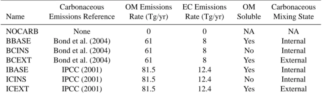
Table 1. Overview of simulations.
Carbonaceous OM Emissions EC Emissions OM Carbonaceous
Name Emissions Reference Rate (Tg/yr) Rate (Tg/yr) Soluble Mixing State
NOCARB None 0 0 NA NA
BBASE Bond et al. (2004) 61 8 Yes Internal
BCINS Bond et al. (2004) 61 8 No Internal
BCEXT Bond et al. (2004) 61 8 Yes External
IBASE IPCC (2001) 81.5 12.4 Yes Internal
ICINS IPCC (2001) 81.5 12.4 No Internal
ICEXT IPCC (2001) 81.5 12.4 Yes External
“mixed” populations, respectively. As pure EC is insoluble, it is not able to activate to CCN. We assume that the mixed EC is itself insoluble but may activate because it is mixed with soluble species. Hydrophobic and hydrophilic OM are assumed to be insoluble and completely soluble, respectively. While representing the entire spectrum of OM species with only two model tracers is a simplification, the mixing rule of the hygroscopicity parameter (κ) in Petters and Kreiden-weis (2007) suggests that any complex organic mixture can be represented by a correctly weighted mixture of a highly hydrophilic group and a highly hydrophobic group (high/low
κ).
Hydrophobic and hydrophilic OM each represent a mix-ture of organic components with varying activation behav-iors. We assume that hydrophilic OM has a critical dry di-ameter of activation of 140 nm at 0.2% supersaturation (the corresponding value of the κ parameter discussed in Pet-ters and Kreidenweis, 2007 is 0.12), a value representative of more hygroscopic organic compounds. The hydrophobic OM was assumed to be insoluble (κ=0). Model simulations that assumed a low solubility (0.01 g per 100 cm3H2O) as
opposed to no solubility were performed, and the resulting CCN(0.2%) concentrations differed by <1%. The assumed density of hydrophilic OM is 1.4 g cm−3 and hydrophobic
OM is 1.8 g cm−3. These values are within the range used in
(Kinne et al., 2003) and the CCN predictions do not depend strongly on the assumed density (it depends more strongly on the moles of solute).
For our mixed aerosol population, we use modified K¨ohler theory to calculate the number of CCN in the model along with the number of active particles in clouds for wet depo-sition (Hanel, 1976; Laaksonen et al., 1998; Raymond and Pandis, 2003; Seinfeld and Pandis, 1998). This allows for the calculation of the activation diameter of particles con-taining various soluble and insoluble (EC and hydrophobic OM) components. The hydrophilic OM contributes the ap-propriate number of solute molecules per OM mass to give an activation diameter of 140 nm at 0.2% supersaturation for a pure hydrophilic OM particle. Sulfate is assumed to be ammonium bisulfate that completely dissociates (van’t Hoff
factor of 3) and sea-salt is assumed to be sodium chloride with a van’t Hoff factor of 2. Hydrophobic OM and all EC are assumed to be an insoluble core. In this treatment, we ignore changes in surface tension due to the contribution of surfactants by the organic aerosol.
In this work, 80% of EC is emitted into the pure EC ulation while the other 20% is added to the mixed EC pop-ulation; half of total primary OM emitted is assumed to be hydrophobic and the other half hydrophilic following Cooke et al. (1999). In the atmosphere, hydrophobic carbonaceous aerosols become hydrophilic by several means: coating by condensation of soluble species such as sulfate or secondary organic aerosols (SOA) (Park et al., 2005; Riemer et al., 2004; Weingartner et al., 1997), coagulation with hydrophilic aerosols (FassiFihri et al., 1997; Riemer et al., 2004; Strom et al., 1992), or by heterogeneous chemistry (Eliason et al., 2003, 2004; FassiFihri et al., 1997; Moise and Rudich, 2002; Park et al., 2005; Riemer et al., 2004; Strom et al., 1992; Weingartner et al., 1997; Zuberi et al., 2005). The time scale for converting hydrophobic carbonaceous aerosols into hy-drophilic aerosols is one of the main factors that affects the wet deposition lifetime of aerosols and thus has significant effect on aerosol mass and number concentrations (Cooke and Wilson, 1996; Park et al., 2005). However, this time scale remains uncertain and previous studies generally as-sume somewhat arbitrary time scales. In previous studies, the assumed time scale has been as low as 1.15 days (Cooke et al., 1999) and as high as 1.8 days (Koch et al., 1999). In this work we assume hydrophobic aerosols convert to hydrophilic aerosols with a lifetime of 1.5 days. This timescale is shorter than the mean lifetime of particles in the atmosphere, so un-certainties in the aging timescale should have only a modest affect on the carbonaceous burden.
In this work we do not consider SOA. Representation of SOA in global aerosol models is a developing field and cur-rent global estimates of SOA have high uncertainty (Kanaki-dou et al., 2005); future work should consider SOA for-mation as it may contribute largely to the carbonaceous mass (Volkamer et al., 2006). It should be noted that the model does underpredict OM mass compared to observations
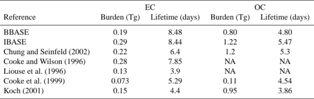
Table 2. Carbonaceous budget information.
EC OC
Reference Burden (Tg) Lifetime (days) Burden (Tg) Lifetime (days)
BBASE 0.19 8.48 0.80 4.80
IBASE 0.29 8.44 1.22 5.47
Chung and Seinfeld (2002) 0.22 6.4 1.2 5.3
Cooke and Wilson (1996) 0.28 7.85 NA NA
Liouse et al. (1996) 0.13 3.9 NA NA
Cooke et al. (1999) 0.073 5.29 0.11 4.54
Koch (2001) 0.15 4.4 0.95 3.86
(Sect. 3.2). The omission of SOA is likely to account for some of this underprediction and thus the contribution of car-bonaceous aerosol to CCN may be underestimated.
2.4 Overview of simulations
The various base case and sensitivity simulations discussed in this paper are summarized in Table 1. All simulations are spun up for six months followed by one year of simulation time. The NOCARB model simulation contains no carbona-ceous aerosol and is the same as the CLRK simulation in Pierce and Adams (2006) with the exception that the aerosol activation cutoff diameters in NOCARB depend on the com-position (ratio of sulfate and sea-salt) according to K¨ohler theory, where in CLRK the cutoff diameters were constant. This does not greatly affect the aerosol burdens and CCN predictions because both sulfate and sea-salt are similarly hygroscopic. BBASE and IBASE are the base case simula-tions for the Bond et al. (2004) and IPCC (2001) emissions, respectively. In these runs, the assumptions about carbona-ceous solubility and aerosol mixing state are as described in the previous sections. In the BCINS and ICINS simulations, the mixing assumptions of the base case runs are the same, but all carbonaceous aerosol is treated as insoluble. These simulations give a lower bound of CCN production with the current emissions in this model due to uncertainty in the sol-ubility of OM and also isolate the effect of carbonaceous seeding on CCN concentrations. The BCEXT and ICEXT simulations use the solubility assumptions of the base cases, but treat four populations as externally mixed during cloud processes: 1) sulfate, 2) sea-salt, 3) hydrophobic OM, hy-drophilic OM and mixed EC and 4) pure EC. The internally mixed carbonaceous are lumped together to simulate car-bonaceous sources that have a mixture of OM and EC. These simulations explore how the mixing state of carbonaceous aerosol with inorganic salts affects CCN concentrations. In the BCEXT and ICEXT simulations, all species are treated as internally mixed during aerosol processes such as coagu-lation, condensation and dry deposition, but externally mixed during cloud processes such as wet deposition and aqueous oxidation. This assumption does not appreciably alter
micro-physical growth rates because condensation and coagulation rates depend primarily on aerosol size, not composition. A second-order effect is the effect of aerosol mixing state on water uptake and, therefore, on condensation and coagulation growth rates. This is a limitation of the current study; nev-ertheless, these sensitivity simulations provide insight about the importance of mixing state on cloud processes.
3 Results and discussion
In this section we will evaluate the model against direct mea-surements of carbonaceous mass and aerosol number con-centrations as well as measurements of the aerosol size distri-bution. This will be followed by a discussion of how primary carbonaceous aerosol affects CCN concentrations as well as an exploration of the importance of aerosol size and compo-sition in predicting CCN. The model is currently unevaluated against satellite and AERONET derived aerosol optical depth (AOD) and angstrom coefficient measurements. This evalua-tion is being performed on an improved version of the model that also includes dust aerosol (Lee et al., 2007a1; Lee et al., 2007b2).
3.1 Aerosol budgets
The burden and lifetime of EC and OM for the two base case runs and various previous publications are given in Table 2. The lifetimes of OM differ between the BBASE and IBASE runs due to the emissions in different regions, whereas the lifetime of EC is the same between the two simulations. The average global burdens for both components are differ-ent between the two simulations due to differdiffer-ent emissions rates. The burden and lifetime values for the BBASE and IBASE simulations are generally within the range of values
1Lee, Y., Chen, K., and Adams, P. J.: Development of a global
model of mineral dust aerosol microphysics, in preparation, 2007a.
2Lee, Y., Chen, K., and Adams, P. J.: Evaluation of a global
aerosol microphysics model against AERONET, MODIS, and MISR measurements of optical depth, in preparation, 2007b.
Table 3. Inorganic budget information.
Sulfate Sea-salt
Simulation Burden (Tg) Lifetime (days) Burden (Tg) Lifetime (days)
NOCARB 0.754 6.12 15.82 0.801
BBASE 0.750 6.08 15.83 0.801
IBASE 0.745 6.05 15.83 0.801
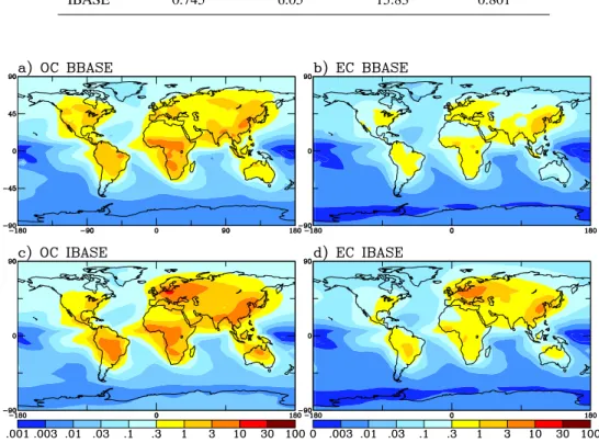
Fig. 1. Annually-averaged mass concentrations of OC (µg C m−3at 298 K and 1 atm) and EC (µg C m−3at 298 K and 1 atm) for BBASE
and IBASE.
presented in the previous work with the EC lifetime being somewhat longer in our model.
Table 3 shows the burden and lifetime of inorganic species in the model without carbonaceous aerosol (NOCARB) and with carbonaceous aerosol (BBASE and IBASE). The sul-fate aerosol shows a very minor decrease in burden and life-time when the carbonaceous aerosol is added. This is likely either due to condensation of sulfate onto the carbonaceous particles, which are emitted at a slightly larger size than pri-mary sulfate particles, or a reduction of nucleation in favor of condensation of existing particles. Both of these shift sulfate mass to larger sizes where they may be removed quickly. The sea-salt aerosol burden and lifetime does not show a change between the simulations because most of the mass is already at large sizes.
3.2 Carbonaceous mass
Figure 1 shows the annual-average OC and EC mass con-centrations for the model surface layer of the BBASE and
IBASE simulations. Note that we present our OC concen-tration as µ g C m−3rather than the total mass of OM to aid
in the comparison to observations presented as OC. We as-sumed an OM:OC ratio of 1.8 for the conversion (El-Zanan et al., 2005; Yu et al., 2005; Zhang et al., 2005). In most re-gions, the IBASE has higher concentrations of both OC and EC than BBASE, especially in Eastern Europe. This is repre-sentative of the differences in the emissions inventories. Two exceptions are higher OC concentrations in western North America and Spain in the BBASE run.
A comparison of OC and EC concentrations to observa-tions are shown in Fig. 2. These are the same observa-tions used in Chung and Seinfeld (2002) that include data from the Interagency Monitoring of Protected Visual En-vironments (IMPROVE) database that consists of approxi-mately 140 rural sites in the United States (Malm et al., 2000) along with various rural, remote and marine sites with loca-tions and references contained in Chung and Seinfeld (2002). Sampling for IMPROVE includes twenty-four hour aerosol samples that were taken twice a week (on Wednesdays and
Table 4. Locations of number concentration measurements used for comparison.
Location Region Reference Time Latitude Longitude Elevation (m) CN (cm−3)
A Aspvereten, Sweden Europe Van Dingenen, et al., 2004 Jan 2001–Dec 2001 58.8 69.4 20 2000
B Harwell, United Kingdom Europe Van Dingenen, et al., 2004 May 1998–Nov 2000 51.6 −1.3 125 3000
C Hohenpeissenberg, Germany Europe Van Dingenen, et al., 2004 Apr 1998–Aug 2000 47.8 11.0 988 2500
D Melpitz, Germany Europe Van Dingenen, et al., 2004 Dec 1996–Nov 1997 51.5 12.9 86 5600
E Ispra, Italy Europe Van Dingenen, et al., 2004 Feb 2000–Dec 2000 45.8 8.6 209 9000
F Thompson Farm, New Hampshire, US North America http://airmap.unh.edu 2001–2005 43.1 −71.0 75 7250
G Lamont, Oklahoma, US North America http://www.cmdl.noaa.gov/aero/data/ 1996–2004 36.5 −97.5 318 5200
H Bondville, Illinois, US North America http://www.cmdl.noaa.gov/aero/data/ 1994–2005 40.1 −88.3 230 3700
I Sable Island, Nova Scotia, Canada North America http://www.cmdl.noaa.gov/aero/data/ 1992–1999 43.9 −60.0 5 850
J Trinidad Head, California, US North America http://www.cmdl.noaa.gov/aero/data/ 2002–2005 41.1 −124.2 107 590
K American Samoa Remote http://www.cmdl.noaa.gov/aero/data/ 1995–2005 −14.2 −170.5 42 220
L South Pole Remote http://www.cmdl.noaa.gov/aero/data/ 1995–2005 −90.0 102.0 2810 100
M Point Barrow, Alaska, US Remote http://www.cmdl.noaa.gov/aero/data/ 1995–2005 71.3 −156.6 11 110
N Mauna Loa, Hawaii, US Free Troposphere http://www.cmdl.noaa.gov/aero/data/ 1995–2005 19.5 −155.6 3397 330
O Jungfraujoch, Switzerland Free Troposphere Van Dingenen, et al., 2004 Jun 1997–May 1998 47.6 8.0 3580 525
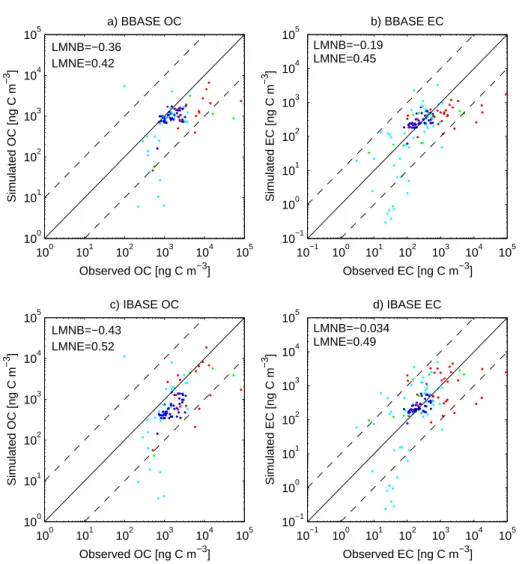
100 101 102 103 104 105 100 101 102 103 104 105 Observed OC [ng C m−3] Simulated OC [ng C m −3 ] a) BBASE OC LMNB=−0.36 LMNE=0.42 10−1 100 101 102 103 104 105 10−1 100 101 102 103 104 105 Observed EC [ng C m−3] Simulated EC [ng C m −3 ] b) BBASE EC LMNB=−0.19 LMNE=0.45 100 101 102 103 104 105 100 101 102 103 104 105 Observed OC [ng C m−3] Simulated OC [ng C m −3 ] c) IBASE OC LMNB=−0.43 LMNE=0.52 10−1 100 101 102 103 104 105 10−1 100 101 102 103 104 105 Observed EC [ng C m−3] Simulated EC [ng C m −3 ] d) IBASE EC LMNB=−0.034 LMNE=0.49
Fig. 2. OC (ng C m−3at 298 K and 1 atm) and EC (ng C m−3at 298 K and 1 atm) mass comparison to observations for BBASE (a and b) and
IBASE (c and d) runs. Solid line shows a 1:1 ratio and dashed line show ratios of 10:1 and 1:10. Sites taken from Chung and Seinfeld (2002). Log-mean normalized bias (LMNB) and log-mean normalized error (LMNE) given on each panel. Blue dots represent comparisons with the IMPROVE database, red dots with rural sites, green with remote sites, and cyan with marine sites (Chung and Seinfeld, 2002). IMPROVE data is a 3 year average and is compared to the 1 year average of the model. The sampling periods of the rural, remote and marine data is given in Tables 10–15 in (Chung and Seinfeld, 2002) and the model is averaged over the same time-period as the sample.
Saturdays). The observation data are averaged over 3 years from March 1996 to February 1999. The sampling of the ru-ral, remote and marine sites are averaged over various time periods and details are given in Tables 10–15 in Chung and Seinfeld (2002). The results of the IBASE simulation are similar to the simulations in Chung and Seinfeld (2002) with the same mass emissions rates in the same host GCM; how-ever Chung and Seinfeld (2002) do not include aerosol size resolution and we use an OM:OC ratio of 1.8 rather than 1.3 in Chung and Seinfeld (2002), so our simulated OC values are approximately 30% smaller. In general, the results for IBASE are similar to that of Chung and Seinfeld (2002), with several locations having observed values more than a factor of ten greater than the simulated values in remote and marine areas. In general, the data in the IMPROVE database falls most closely to the 1:1 line and better agreement is shown for the EC than for OC. The BBASE simulation shows better agreement for OC with the IMPROVE database due to the higher levels of OM in the western United States. It should be noted that the methods for quantifying BC/EC for the ob-servations networks and the emissions inventories vary by a factor of two (Andreae and Gelencser, 2006; Heintzenberg et al., 2006; Subramanian et al., 2006).
To assess the comparison, the log-mean normalized bias (LMNB) and log-mean normalized error (LMNE) for the comparisons (data from all networks lumped together) are included on each panel. The simulations using both invento-ries are biased low for OC with LMNB of −0.36 and −0.46 corresponding to underpredictions by factors of 2.3 and 2.9 for the BBASE and IBASE simulations. The predictions of EC are less biased with LMNB of −0.19 and −0.034 corre-sponding to underpredictions by factors of 1.5 and 1.1 for the BBASE and IBASE simulations. The LMNE for all simula-tions are similarly high, between 0.42 and 0.52. This means that the model predictions are, on average, within observed values to a factor of 3.
3.3 Aerosol number
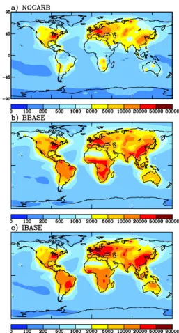
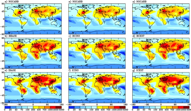
Figure 3 shows the annual-average predicted aerosol number (condensation nuclei, CN) concentration (cm−3with 10 nm
lower cutoff) for the model surface layer from the NOCARB, BBASE and IBASE simulations. The changes in CN con-centration due to addition of carbonaceous aerosol is the dif-ference between the BBASE or IBASE simulation and the NOCARB simulation. The largest increases in aerosol num-ber occur in the biomass burning regions of tropical South America, Africa and Southeast Asia. The addition of pri-mary carbonaceous aerosol in these regions causes CN pre-diction to increase by more than a factor of 20 in some places. Recent work, however, suggests that CN concentrations in these areas may be overpredicted, as the size distribution of primary particles from biomass burning more likely have a number median diameter on the order of 100 nm rather than the 25 nm number median diameter used here (Rissler et al.,
Fig. 3. Annually-averaged CN concentrations (cm−3at 298 K and
1 atm) for NOCARB, BBASE and IBASE simulations.
2004; Rissler et al., 2006). Other notable increases in CN occur in polluted regions, particularly India and China where CN increase by a factor of 2–5 with the addition of the pri-mary carbonaceous aerosol. Not shown in Fig. 3 is the sen-sitivity of CN concentrations to the assumptions about mix-ing state and organic solubility (BCEXT, ICEXT, BCINS, and ICINS simulations). The CN concentrations were quite insensitive to these assumptions with no more than a 10% change in CN in any model grid cell and less than a 1% change in CN globally averaged.
We have assembled a set of long-term CN observations to compare to our simulations, shown in Table 4. The data we have chosen was restricted to sites outside of urban areas with a minimum sample time of about one year. The sites included are part of a European network of sites presented in Van Dingenen et al. (2004), the Global Monitoring Division (GMD) of the Earth Systems Research Laboratory (Schnell, 2003) (http://www.esrl.noaa.gov/gmd/) and the Thompson Farm site of AIRMAP (http://airmap.unh.edu/). The CN ob-servations were done using a condensation nucleus counter (CNC) in the case of the GMD and AIRMAP data and us-ing a CNC with various size scannus-ing devices in the case of the European sites. The low limit cutoff for the CNCs in
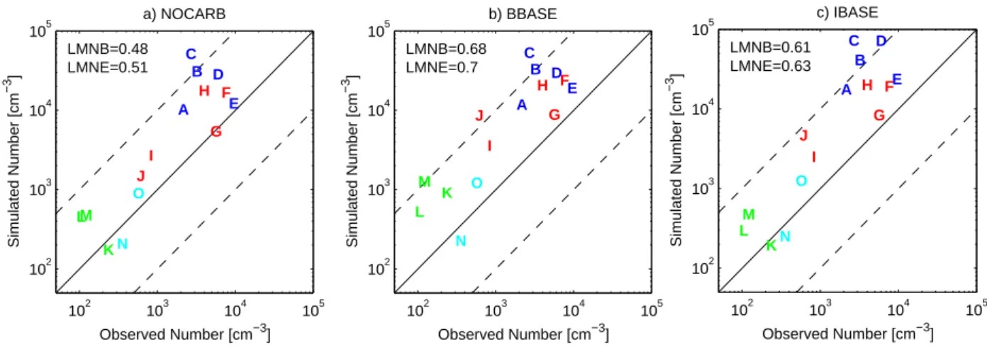
102 103 104 105 102 103 104 105 Observed Number [cm−3] Simulated Number [cm −3 ] a) NOCARB A B C D E F G H I J K LM N O LMNB=0.48 LMNE=0.51 102 103 104 105 102 103 104 105 Observed Number [cm−3] Simulated Number [cm −3 ] b) BBASE A B C D E F G H I J K L M N O LMNB=0.68 LMNE=0.7 102 103 104 105 102 103 104 105 Observed Number [cm−3] Simulated Number [cm −3 ] c) IBASE A B C D E F G H I J K L M N O LMNB=0.61 LMNE=0.63
Fig. 4. Comparison of simulated aerosol number concentrations to observed number concentrations for (a) NOCARB, (b) BBASE and (c)
IBASE simulations (cm−3at 298 K and 1 atm). Solid line shows a 1:1 ratio and dashed line show ratios of 10:1 and 1:10. The letters refer
to the locations presented in Table 3. Blue letters refer to European sites. Red letters refer to North American sites. Green letters refer to remote sites. Cyan letters refer to free tropospheric sites. Log-mean normalized bias (LMNB) and log-mean normalized error (LMNE) given on each panel.
the GMD and AIRMAP data is 10 nm (which corresponds to the lower size limit of the model). The lower size limit for the CNCs used in the Van Dingenen et al. (2004) paper vary, however, they have corrected their number counts for a lower cutoff of 10 nm using the size distribution measurements. The comparison of CN measured at these sites to the NO-CARB, BBASE and IBASE simulation results is shown in Fig. 4. The log-mean normalized bias (LMNB) and log-mean normalized error (LMNE) for the comparisons are included on each panel. In general, the model tends to overpredict the CN concentrations in these areas even without carbonaceous aerosol included. The LMNB for the NOCARB run is 0.48 so on average the model overpredicts by a factor of 100.48 or 3. This may be a consequence of the assumption that 3% of sulfur mass from anthropogenic emissions is assumed to be emitted as aerosol sulfate with ultrafine sizes (Adams and Seinfeld, 2003). In Adams and Seinfeld (2002), it was shown that most of the CN in polluted regions of the model is from primary sulfate rather than from nucleation. This implies that either too much of the sulfate mass is being emitted as pri-mary sulfate or the pripri-mary sulfate particles are emitted at sizes that are too small. Adding primary carbonaceous emis-sions has a range of impacts on predicted CN concentrations from no change to increases of more than a factor of 5 at a given site. Because the NOCARB simulation already over-predicted CN, the addition of primary carbonaceous aerosol causes the model to overpredict further CN concentrations in some areas. The LMNB for the BBASE and IBASE runs are 0.68 and 0.61 corresponding to average overpredictions by factors of 4.8 and 4.1, respectively. The LMNE is essen-tially the same as the LMNB for each simulation because the model overpredicts aerosol number at nearly every location. In the small number of comparisons shown, the IBASE
simu-lation predicted the concentrations of remote and free tropo-spheric areas more accurately than polluted areas, whereas this trend is not as clear in the BBASE simulations. This may be due to the increase in emissions from developing ar-eas in the Bond et al. (2004) inventory. The bias in CN by the model is large and we are currently addressing this in our future work.
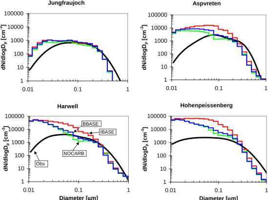
In order to determine if the model is representing the CCN concentrations more accurately than CN concentrations, we have done comparisons of the aerosol size distribution. Fig-ures 5 and 6 show a comparison of simulated to observed aerosol number size distributions at four of the locations (Jungfraujoch, Aspvreten, Harwell and Hohenpeissenberg) from Van Dingenen et al. (2004) and Putaud et al. (2003) for June, July and August, and December, January and February, respectively. Both simulations and observations show the number size distribution as a function of dry diameter with the exception of the observations at Harwell, which are given as ambient diameter. The data in Van Dingenen et al. (2004) is given as average distributions for the morning, afternoon and night. We have plotted the mean values of these three distributions. The total number at all four locations were shown to be overpredicted in all model simulations in Fig. 4. Figures 5 and 6 are consistent with this with the NOCARB, BBASE and IBASE simulations overpredicting the aerosol number in the ultrafine (Dp<100 nm) size range. The three
simulations predict the size distributions more accurately for sizes larger than 100 nm. CCN(0.2%) are, in general, par-ticles of about 80–100 nm and larger, giving us confidence that our model is predicting CCN at these European locations more accurately than the model is predicting CN. Also shown in Figs. 5 and 6 is that the dominating number mode at these locations for all simulations is centered around 20 nm. This
Aspvreten 1 10 100 1000 10000 100000 0.01 0.1 1 µµµµm d N /d lo g Dp [ c m -3 ] Jungfraujoch 1 10 100 1000 10000 100000 0.01 0.1 1 µµµµm d N /d lo g Dp [ c m -3 ] Hohenpeissenberg 1 10 100 1000 10000 100000 0.01 0.1 1 Diameter [µµµµm] d N /d lo g Dp [ c m -3 ] Harwell 1 10 100 1000 10000 100000 0.01 0.1 1 Diameter [µµµµm] d N /d lo g Dp [ c m -3 ] Obs NOCARB IBASE BBASE
Fig. 5. Comparison of simulated number distributions to observations at four European locations published in Van Dingenen et al. (2004) and Putaud et al. (2003) for June, July and August. The x-axis is dry diameter for both the model and observations, except for the observations at Harwell which is ambient diameter. The observational data was published as a fit to three lognormal modes for morning, afternoon and night. We have plotted the mean of these three distributions.
corresponds approximately to the primary sulfate emission size, and because we do not get significant boundary layer nucleation, this is likely a major source of the CN overesti-mation. We are improving the ultrafine distribution as part of our future work.
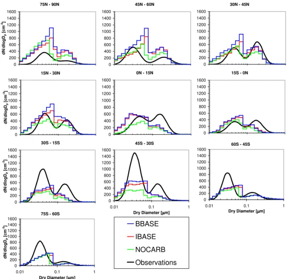
Figure 7 shows a comparison of predicted marine number size distributions from the NOCARB, BBASE and IBASE simulations with observations compiled in Heintzenberg et al. (2000). Heintzenberg et al. (2000) collected a large set of observations of marine aerosol size distributions and summa-rized them by fitting the aerosol number distributions to two lognormal modes for each latitudinal zone. These data came from a wide array of sampling sites and field campaigns and used many different sampling instruments. The latitudinal bands are 15◦wide with no data between 75◦S–90◦S and
60◦N–75◦N. The 15◦by 15◦grid cells from which the data
were obtained is presented in their Fig. 1. Rather than using all ocean grid cells for comparison, we generally used model results from the same 15◦by 15◦regions where observations
were collected. However, some of the 15◦ by 15◦grid
ar-eas include continental arar-eas (e.g. observations from Mace Head, Ireland are in the same 15◦by 15◦grid cell as most of
the British Isles). Because the GCM grid resolution is finer, we exclude these continental sub-areas from our comparison
as they greatly increase (and bias) ultrafine number concen-trations. For the 0◦to 15◦N, we used the model predicted
av-erage values from the wet season (June–August), when these particular observations were taken, to remove biomass burn-ing influence from the marine aerosol.
Figure 7 shows that, in most latitude bands, the model does a good job of representing the bimodal size distribution rep-resented by the Heintzenberg et al. (2000) data. Through-out most the Northern Hemisphere and also in the 45◦S–
30◦S latitude band, the addition of carbonaceous particles
increases the number of particles significantly; throughout the rest of the Southern Hemisphere the contribution of car-bonaceous aerosol is minor. Moreover, it can be seen that the “Hoppel Gap” between the two modes of the distribution shifts toward larger sizes in the simulations with carbona-ceous aerosol. The location of the Hoppel Gap depends on the average activation diameter, so this shift is the direct re-sult of the mixed carbonaceous/sulfate/sea-salt particles be-ing somewhat less hygroscopic than the sulfate/sea-salt only particles. This influence on the activation diameter can be seen even in the southernmost latitude bands. In Fig. 7, all of the simulations overpredict at the North Pole, underpredict in the Southern Hemisphere and compare best in the Northern Hemisphere mid-latitude bands. Averaging over all latitude
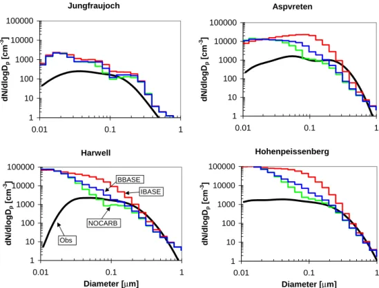
Aspvreten 1 10 100 1000 10000 100000 0.01 0.1 1 µm dN /dlogD p [cm -3 ] Jungfraujoch 1 10 100 1000 10000 100000 0.01 0.1 1 µm dN /dlogD p [cm -3 ] Hohenpeissenberg 1 10 100 1000 10000 100000 0.01 0.1 1 Diameter [µm] dN/ d logD p [c m -3 ] Harwell 1 10 100 1000 10000 100000 0.01 0.1 1 Diameter [µm] dN /dlogD p [cm -3 ] Obs NOCARB IBASE BBASE
Fig. 6. Comparison of simulated number distributions to observations at four European locations published in Van Dingenen et al. (2004) and Putaud et al. (2003) for December, January and February. The x-axis is dry diameter for both the model and observations, except for the observations at Harwell which is ambient diameter. The observational data was published as a fit to three lognormal modes for morning, afternoon and night. We have plotted the mean of these three distributions.
bands, the BBASE simulation overpredicts total number by 30%, the IBASE overpredicts by 15% and the NOCARB simulation underpredicts by 10%. This contrasts with the results shown in Fig. 4, where the model largely overpredicts the total number of particles in most areas. It is possible that because these marine areas are away from large primary par-ticle sources, the overprediction of parpar-ticles near sources has been dampened by aerosol number removal processes such as coagulation and deposition.
3.4 Cloud condensation nuclei
In this section we explore CCN predictions by the model and test the sensitivity of CCN to organic solubility and mixing assumptions. Although the model overpredicted CN glob-ally, the model showed much less bias in the accumulation mode number in Figs. 5 through 7. Furthermore, CCN con-centrations tend to vary sub-linearly with CN concon-centrations allowing CCN errors to be, in general, smaller than CN er-rors.
The annual-average CCN concentrations at 0.2% super-saturation (CCN(0.2%)) for the model surface level of the NOCARB, BBASE, BCINS, BCEXT, IBASE, ICINS and ICEXT simulations are shown in Fig. 8. The CCN(0.2%) concentrations are found using modified K¨ohler theory as
discussed earlier with the annually averaged size distribu-tions and chemical composidistribu-tions. Using average size dis-tributions and compositions to calculate average CCN con-centrations rather than using the average of the instantaneous CCN concentrations gave results with error on the order of 2% globally when tested across a three month period. The addition of the Bond et al. (2004) primary carbonaceous emissions to the NOCARB model simulation (BBASE) in-creases CCN(0.2%) by 65% globally averaged. The addition of the IPCC (2001) primary carbonaceous emissions to the NOCARB model simulation (IBASE) increases CCN(0.2%) by 89% globally averaged. The differences in CCN(0.2%) between the BBASE and IBASE are notable in eastern Eu-rope and the Amazon basin where IBASE predicts higher CCN(0.2%) concentrations and in western North America where BBASE predicts higher CCN(0.2%) concentrations. These results confirm that, for the base case assumptions, the contribution of primary carbonaceous aerosol is quite large and cannot be ignored. However, it is unclear from the base case simulations alone how much the increase in CCN from primary carbonaceous aerosol comes from the ad-dition of new particles (carbonaceous seeding effect) verses the addition of more solute (organic solute effect). To under-stand this, we look at the sensitivity of our predicted CCN to
30N - 45N 0 200 400 600 800 1000 1200 1400 1600 0.01 0.1 1 µ µ µ µm d N /d ln D p ( c m -3) 45N - 60N 0 200 400 600 800 1000 1200 1400 1600 0.01 0.1 1 µ µ µ µm d N /d ln D p ( c m -3) 15S - 0N 0 200 400 600 800 1000 1200 1400 1600 0.01 0.1 1 Dry Diameter [µµµµm] d N /d ln D p ( c m -3) 75N - 90N 0 200 400 600 800 1000 1200 1400 1600 0.01 0.1 1 µ µ µ µm d N /d lo g Dp [ c m -3] 0N - 15N 0 200 400 600 800 1000 1200 1400 1600 0.01 0.1 1 µ µµ µm d N /d ln D p ( c m -3) 15N - 30N 0 200 400 600 800 1000 1200 1400 1600 0.01 0.1 1 µ µµ µm d N /d lo g Dp [ c m -3] 45S - 30S 0 200 400 600 800 1000 1200 1400 1600 0.01 0.1 1 Dry Diameter [µµµm]µ d N /d ln D p ( c m -3) 30S - 15S 0 200 400 600 800 1000 1200 1400 1600 0.01 0.1 1 Dry Diameter [µµµµm] d N /d lo g Dp [ c m -3] 60S - 45S 0 200 400 600 800 1000 1200 1400 1600 0.01 0.1 1 Dry Diameter [µµµµm] 75S - 60S 0 200 400 600 800 1000 1200 1400 1600 0.01 0.1 1 Dry Diameter [µµµµm] d N /d lo g Dp [ c m -3] 0 100 200 300 400 500 600 700 800 900 0.01 0.1 1 µ µ µ µm d N /d ln D p ( c m -3) BBASE IBASE NOCARB Observations
Fig. 7. Comparison of simulated number distributions in oceanic regions to observations published in Heintzenberg et al. (2000) all data at 298 K and 1 atm. The model size distributions are averaged over the oceanic grid cells where the observations occurred and are
annually-averaged with the exception of 0◦to 15◦N in which the aerosol is sample over (June–August) when the observations were taken.
organic solubility. The sensitivity of the number of CCN to the mixing assumptions is also explored.
3.4.1 Sensitivity to OM solubility
We tested the sensitivity of model predictions to the base case assumptions of organic solubility by assuming that all car-bonaceous aerosol is insoluble in the BCINS and the ICINS simulations (see Sect. 2.4). This simultaneously gives infor-mation about the relative magnitudes of the “carbonaceous seeding effect” and the “organic solute effect” because the “organic solute effect” is turned off. The CCN(0.2%) pre-dicted by the BCINS and ICINS are shown in Fig. 8. For the simulations using the Bond et al. (2004) carbonaceous emissions, the global-average CCN(0.2%) concentration in-creased from 193 cm−3 to 268 cm−3 (at 1 bar and 293 K)
by adding insoluble carbonaceous particles to the NOCARB simulation. By allowing most of the organics to be soluble (with the hygroscopic properties discussed in Sect. 2.3) in the BBASE run, the global-average CCN(0.2%) concentra-tion increases to 320 cm−3. This shows that for the solubility
assumptions used in the BBASE run, “carbonaceous seed-ing” accounts for just over half of carbonaceous aerosol’s globally averaged contribution to CCN while the “organic so-lute” accounts for the remainder. This fraction varies region-ally, however. In areas with large amounts of carbonaceous emissions compared to inorganics, such as central Africa, the effect of carbonaceous seeding is more modest (20–40%) in the BCINS and ICINS simulations because there is not enough inorganic aerosol to condense onto the insoluble car-bonaceous particles to make them CCN active. Conversely, in regions with an abundance of sulfur emissions such as
Fig. 8. Annually-averaged CCN concentrations at 0.2% supersaturation (cm−3at 298 K and 1 atm) for the surface layer for the NOCARB,
BBASE, BCEXT, IBASE, ICINS and ICEXT simulations.
the western United States or Western Europe, the “carbona-ceous seeding effect” dominates the increase of CCN from carbonaceous emissions (responsible for >70% of CCN en-hancement by carbonaceous aerosol). Similar results are found for the simulations using the IPCC (2001) carbona-ceous emissions. The global-average CCN(0.2%) increased from 193 cm−3 to 295 cm−3 by adding insoluble
carbona-ceous particles to the NOCARB simulation. By allowing carbonaceous aerosol to be soluble (with the hygroscopic properties discussed in Sect. 2.3) in the IBASE run the CCN(0.2%) increased to 365 cm−3. In this globally
aver-aged case, “carbonaceous seeding” again accounts for just over half of the increase in CCN(0.2%) due to carbonaceous particles.
There is a relatively large uncertainty in the solubility and ionic nature of organic matter (Kanakidou et al., 2005); how-ever, varying the solubility/hygroscopicity of organic matter in these simulations from largely soluble to completely in-soluble changed the number of CCN(0.2%) predicted by the simulations by less than 20% globally averaged, with up to 50% reductions in biomass burning areas and smaller reduc-tions in high sulfate areas. The range of uncertainty in or-ganic solubility and ionic ability explored here likely spans beyond the range of the real atmosphere. With this we would expect that the uncertainty in CCN(0.2%) due to uncertainty
in organic solubility is significantly less than 20%.
3.4.2 Sensitivity to mixing assumption
In the BCEXT and ICEXT simulations we assume that the carbonaceous aerosol is externally mixed during wet removal processes (see Sect. 2.4). The four populations are, however, still assumed to be internally mixed during aerosol micro-physical processes so their sizes may change due to coagula-tion, condensation and aqueous oxidation. The CCN(0.2%) concentrations of these two simulations are shown in Fig. 8. For both emissions sets, the externally mixed cases show slightly higher CCN(0.2%) concentrations than the base case scenarios. This happens because for most of the aerosol distributions predicted by the model, assuming the particles are externally mixed when calculating CCN(0.2%) yields approximately the same number of CCN as assuming that the particles are internally mixed. This is shown by ap-plying the externally mixed assumption to calculate the CCN(0.2%) from BBASE and IBASE size distributions and chemical compositions offline rather than using the internally mixed assumption. In doing this the CCN(0.2%) changes from 320 cm−3 to 318 cm−3 for BBASE and 365 cm−3 to
354 cm−3for IBASE. Another reason why the BBASE and
0 1000 2000 3000 0 1000 2000 3000 a) Average composition CCN(0.2%) from GCM CCN(0.2%) with assumption 0 1000 2000 3000 0 1000 2000 3000 b) Average size−distribution CCN(0.2%) from GCM CCN(0.2%) with assumption 0 1000 2000 3000 0 1000 2000 3000 c) Bulk mass CCN(0.2%) from GCM CCN(0.2%) with assumption
Fig. 9. (a) Model surface layer comparison of BBASE CCN(0.2%) with CCN(0.2%) simulated from BBASE assuming a globally average composition as a function of size and the size distribution varies spatially (annual average for each grid cell in the lowest model layer). (b) Comparison of BBASE CCN(0.2%) with CCN(0.2%) simulated from BBASE assuming a globally average size distribution and the size dependent chemical composition varies spatially(annual average for each grid cell in the lowest model layer). (c) Comparison of BBASE CCN(0.2%) with CCN(0.2%) simulated from BBASE assuming the globally averaged sized distribution of each species scaled by the total mass of those species in each grid cell (annual average for each grid cell in the lowest model layer).
have similar CCN predictions is because the aerosols are not assumed to be externally mixed during aerosol microphysical processes. This means that ultrafine carbonaceous aerosol may grow in size to sizes where the carbonaceous aerosol will activate to form CCN whereas if it were truly externally mixed this would not occur.
These results have shown that, for the assumptions made in the model, the number of CCN in areas well mixed and away from sources does not greatly depend on the mixing assumption as long as OM is soluble. If the hygroscopicity of the carbonaceous particles is reduced, then the number of CCN will approach the NOCARB results as the hygroscop-icity/solubility is reduced to zero.
3.5 Aerosol size distribution versus aerosol composition
K¨ohler theory and observations (Dusek et al., 2006) indi-cate that knowing the size distribution is more important than knowing the chemical composition when predicting CCN concentrations. While Dusek et al. (2006) showed that time variability in aerosol composition at their measurement site in Germany had little effect on CCN concentrations, we use our model predictions to test the importance of regional variability in aerosol composition. Specifically, we will ex-plore the error in CCN prediction that occurs when assuming global-average chemical composition or global-average size distributions rather than using location-specific information about both. All data used in this section are taken from the BBASE simulation.
For Fig. 9a, we calculated the global-average chemical composition as a function of size across the lowest model layer and used it with the predicted size distribution in each grid cell to predict the number of CCN(0.2%) (cm−3) in
that grid cell. In Fig. 9a we have plotted these CCN pre-dictions versus the CCN prepre-dictions using the size distribu-tion and chemical composidistribu-tion predicted for each grid cell (Fig. 8b). In general, the CCN(0.2%) calculated using the global-average chemical composition agrees within a factor of two with the CCN(0.2%) calculated using no averaging. This is a much wider range of error than shown in Dusek et al. (2006) due to the wider range of compositions in the model than in the test region of Dusek et al. (2006). The areas where the CCN(0.2%) with average chemical compo-sition overpredict are areas with large amounts of less CCN-active carbonaceous particles such as the biomass burning in-fluenced tropical regions. In these regions the average ical composition is more CCN active than their actual chem-ical composition. Conversely, regions where the CCN(0.2%) with average chemical composition underpredict are areas with large amounts of inorganic species.
For Fig. 9b, we calculated the global-average size distribu-tion across the lowest model layer and used it with the pre-dicted chemical composition (as a function of size) in each grid cell to predict the number of CCN(0.2%) (cm−3) in that
grid cell. We plotted these values against the CCN predic-tions using the size distribution and chemical composition predicted for each grid cell (Fig. 8b). The CCN(0.2%) us-ing the global-average size distribution vary only between about 200 cm−3and 600 cm−3, whereas the CCN(0.2%)
pre-dicted not using the global-averaging range from 0 cm−3to
3000 cm−3. There is essentially no correlation between the
two data sets. The areas with much more sea-salt aerosol than carbonaceous aerosol appear on the high end of the CCN(0.2%) prediction with the global average size distribu-tions, even when their total number of particles is actually very low, such as southern hemisphere marine environments.
On the other hand, areas that have large amounts of aerosol but a large portion of if its mass is carbonaceous aerosol, such as the tropical biomass burning regions, will have the lowest predicted CCN(0.2%) in the global-average size distribution calculation.
Figure 9c shows an additional comparison to evaluate the ability of global models without microphysics (bulk aerosol models) to calculate CCN. In this figure, we compare the BBASE CCN(0.2%) to CCN(0.2%) calculated assuming that the shape of the size distribution of each of the six chemical species or groups is the same as the globally averaged size-distribution of those species, but is scaled by the total mass of each species in each grid cell. This is similar to GCM simulations that calculate the total mass of each species and then assume a size distribution of each species when calcu-lating the CCN. Figure 9c shows that the “bulk mass” model agrees with the BBASE CCN(0.2%) with a normalized error of 35%. This shows that bulk models can, in general, cal-culate the general spatial distribution of CCN(0.2%). There are, however, other reasons why microphysical models are advantageous over bulk models. Although the size distribu-tion of particles for the current time period may be measured, this is not the case of past or future time periods where the size distributions may be different. The relative contribution of primary particles and nucleated particles to CN and CCN may be explored using microphysical models but cannot be in bulk models.
Obviously there are major differences between this analy-sis and the one shown in (Dusek et al., 2006); however, both clearly show it is impossible to predict CCN concentrations without an accurate size distribution. In contrast to that work, these results suggest that regional variability in aerosol com-position are important in predicting CCN. In our case, up to a factor of two error is introduced when a (size-dependent) chemical composition is assumed.
4 Conclusions
We explored the impact of primary carbonaceous aerosol on cloud condensation nuclei (CCN) concentrations in a global climate model with online size-resolved aerosol mi-crophysics. Two emissions inventories of organic matter (OM) and elemental carbon (EC) were tested in the model along with sulfate and sea-salt aerosol. Simulations were run with various assumptions of the solubility and mixing state of the carbonaceous aerosol to provide bounds on its impacts on CCN concentrations.
Predicted primary carbonaceous aerosol mass and aerosol number concentrations were compared to observations. Er-rors in predictions of OC and EC masses were a factor of 3 on average and OC predictions were biased towards too lit-tle mass whereas EC predictions showed litlit-tle bias. A com-parison to a network of total aerosol number measurements shows that the model predicted number concentrations were
on average about a factor of 4 too high. Even without car-bonaceous particles included, the number concentrations are already factor of 3 too high. A comparison of the simulated aerosol size distributions to observations at several European sites showed that the overprediction of CN at these sites was due to large overpredictions in the number of particles with diameters smaller than 100 nm, whereas the accumu-lation mode particles were predicted much more accurately. This overprediction of CN may be due to the emission of too many particles through primary sulfate emissions and aided by incorrect emission size distributions of carbonaceous par-ticles. In contrast, a comparison of CN to marine observa-tions showed very little overprediction (<30%). The sensi-tivity of CN and CCN to these emissions is being performed in future work.
It was found that adding primary carbonaceous aerosol increased CCN(0.2%) concentrations by 65–90%, depend-ing on which emissions dataset was used, compared with a model with sulfate and sea-salt aerosol only. The largest in-creases in CCN(0.2%) occurred in the biomass burning re-gions of South America and Africa and in rere-gions of eastern Asia and Australia. Assuming that all carbonaceous aerosol is insoluble, rather than mostly soluble in our base case, the carbonaceous aerosol still increases CCN(0.2%) by 40–50% over the sulfate/sea-salt only simulation. This shows that around half of the increase in CCN due to primary carbona-ceous aerosol occurs due to the addition of new aerosol par-ticles (seeding effect) where the CCN are created by regard-less of carbonaceous solubility/hygroscopicity (because the carbonaceous particles end up coated with hydrophilic mate-rial). The other half of the CCN generated by carbonaceous aerosol depends on carbonaceous solubility/hygroscopicity (solute effect). The solute effect tends to dominate (respon-sible for >70% of the carbonaceous CCN) more in areas where there is less inorganic aerosol than organic aerosol, such as biomass burning regions, and the seeding effect tends to dominate in areas where is more inorganic aerosol than or-ganic aerosol, such as eastern North America. The effect of the assumption of internal versus external mixing of the car-bonaceous aerosol with inorganic aerosol during cloud pro-cesses was found to have little effect on the number of CCN generated as long as the carbonaceous aerosol was mostly soluble.
To evaluate the importance of chemical composition and the aerosol size distribution globally, we calculate the CCN(0.2%) in each grid cell by using globally averaged chemical composition or globally averaged size distributions. We found that, in general, the CCN(0.2%) calculated by assuming a uniform globally averaged chemical composi-tion for the entire globe (while using the predicted size dis-tribution in each location) was within a factor of 2 of the CCN(0.2%) calculated with both chemical composition and size distribution information. The CCN(0.2%) calculated from assuming a uniform globally averaged size distribu-tion for the entire globe (while using the predicted