HAL Id: hal-00090011
https://hal.archives-ouvertes.fr/hal-00090011
Submitted on 25 Aug 2006
HAL is a multi-disciplinary open access
archive for the deposit and dissemination of
sci-entific research documents, whether they are
pub-lished or not. The documents may come from
teaching and research institutions in France or
abroad, or from public or private research centers.
L’archive ouverte pluridisciplinaire HAL, est
destinée au dépôt et à la diffusion de documents
scientifiques de niveau recherche, publiés ou non,
émanant des établissements d’enseignement et de
recherche français ou étrangers, des laboratoires
publics ou privés.
Chemical sensitivity to the ratio of the cosmic-ray
ionization rates of He and H2 in dense clouds
Valentine Wakelam, Eric Herbst, Franck Selsis, Gérard Massacrier
To cite this version:
Valentine Wakelam, Eric Herbst, Franck Selsis, Gérard Massacrier. Chemical sensitivity to the ratio
of the cosmic-ray ionization rates of He and H2 in dense clouds. Astronomy and Astrophysics - A&A,
EDP Sciences, 2006, 459, pp.813-820. �hal-00090011�
ccsd-00090011, version 1 - 25 Aug 2006
Astronomy & Astrophysicsmanuscript no. 5472.hyper31651 c ESO 2006
August 25, 2006
Chemical sensitivity to the ratio of the cosmic-ray ionization rates
of He and H
2
in dense clouds
V. Wakelam
1,2, E. Herbst
1,3, F. Selsis
4, and G. Massacrier
41 Department of Physics, The Ohio State University, Columbus, OH 43210, USA
2 Observatoire Aquitain des Sciences de l’Univers, Laboratoire d’Astrodynamique, d’Astrophysique et d’A´eronomie de Bordeaux, CNRS/INSU UMR 5804, BP 89, 33270 Floirac, France
3 Departments of Astronomy and Chemistry, The Ohio State University, Columbus, OH 43210, USA
4 Ecole Normale Sup´erieure de Lyon, Centre de Recherche Astronomique de Lyon, 46 all´ee d’Italie, 69364 Lyon Cedex 07, France ; CNRS, UMR 5574 ; Universit´e de Lyon 1, Lyon, France.
Received 21 April 2006 / Accepted 9 August 2006
ABSTRACT
Aims.To determine whether or not gas-phase chemical models with homogeneous and time-independent physical conditions explain the many observed molecular abundances in astrophysical sources, it is crucial to estimate the uncertainties in the calculated abundances and compare them with the observed abundances and their uncertainties. Non linear amplification of the error and bifurcation may limit the applicability of chemical models. Here we study such effects on dense cloud chemistry.
Methods. Using a previously studied approach to uncertainties based on the representation of rate coefficient errors as log normal distributions, we attempted to apply our approach using as input a variety of different elemental abundances from those studied previously. In this approach, all rate coefficients are varied randomly within their log normal (Gaussian) distribution, and the time-dependent chemistry calculated anew many times so as to obtain good statistics for the uncertainties in the calculated abundances.
Results. Starting with so-called “high-metal” elemental abundances, we found bimodal rather than Gaussian like distributions for the abundances of many species and traced these strange distributions to an extreme sensitivity of the system to changes in the ratio of the cosmic ray ionization rate ζHe for He and that for molecular hydrogen ζH2. The sensitivity can be so extreme as to cause a region of bistability,
which was subsequently found to be more extensive for another choice of elemental abundances. To the best of our knowledge, the bistable solutions found in this way are the same as found previously by other authors, but it is best to think of the ratio ζHe/ζH2as a control parameter
perpendicular to the ”standard” control parameter ζ/nH.
Key words. Astrochemistry – ISM: abundances – ISM: clouds – ISM: molecules
1. Introduction
The equations describing the chemical evolution of quiescent cores (also known as molecular clouds) are highly non-linear and can result in extreme sensitivity to the initial conditions or to some of the parameters. For example, the elemental ratio of carbon to oxygen is well known to be an important parameter for dense cloud chemistry (Terzieva & Herbst 1998). Another well-known consequence of this non-linearity is the presence of bistable regions for some ranges of model parameters (tem-perature, density, comic-ray ionization rate, rate coefficients and elemental abundances). The phenomenon of bistability is characterized by two stable solutions for chemical abundances at steady-state for the same set of parameters. Bistability in
Send offprint requests to: V. Wakelam, e-mail:
dark cloud conditions, i.e. at low temperature, was first discov-ered by Le Bourlot et al. (1993) and subsequently studied by a large number of authors (Le Bourlot et al. 1995; Shalabiea & Greenberg 1995; Lee et al. 1998; Pineau Des Forˆets & Roueff 2000; Charnley & Markwick 2003; Boger & Sternberg 2006). The two solutions of this bistability are characterized by a large difference in the C/CO and O/O2 ratios and in the ionization
fraction. For this last reason, they were named the High and Low Ionization Phases (HIP and LIP). Le Bourlot et al. (1995) showed that the region of bistability can be mapped out by variations in density, temperature, cosmic-ray ionization rate, and elemental depletions within specific ranges. Pineau Des Forˆets & Roueff (2000) later showed that even variations in rate coefficients can lead to the two solutions. Recently, Boger & Sternberg (2006) identified the chemical mechanisms of this phenomenon as a cycle involving the H+3, O2, and S+species.
2 V. Wakelam et al.: Extreme sensitivity of the dense cloud chemistry
Table 1. High- and low- metal elemental abundances with
re-spect to H2.
Element High-Metal Low-Metal (Intermediate) He 2.8 × 10⁻¹ 2.8 × 10⁻¹ N 4.28 × 10⁻⁵ 4.28 × 10⁻⁵ O 3.52 × 10⁻⁴ 3.52 × 10⁻⁴ C+ 1.46 × 10⁻⁴ 1.46 × 10⁻⁴ S+ 1.6 × 10⁻⁵ 1.6 × 10⁻⁷ (2.0 × 10⁻⁶) Si+ 1.6 × 10⁻⁶ 1.6 × 10⁻⁸ Fe+ 6.0 × 10⁻⁷ 6.0 × 10⁻⁹ Na+ 4.0 × 10⁻⁷ 4.0 × 10⁻⁹ Mg+ 1.4 × 10⁻⁷ 1.4 × 10⁻⁸ P+ 6.0 × 10⁻⁷ 6.0 × 10⁻⁹ Cl+ 8.0 × 10⁻⁷ 8.0 × 10⁻⁹
Note: The intermediate-metal case differs from the low-metal case by the S+abundance only, as is indicated in brackets in the table.
In two previous papers, we presented a Monte Carlo method to compute the theoretical error of abundances in chemical models due to uncertainties in rate coefficients and physical conditions (Wakelam et al. 2005, 2006). The errors in the rate coefficients are defined by a log-normal distribution. As a consequence, the resulting abundances at steady-state usually follow a Gaussian distribution (Wakelam et al. 2005). When applying this method, we found that the chemical abundances are very sensitive to the ratio between the ionization rates of helium ζHe and molecular hydrogen ζH2 caused by cosmic-ray
particles. Characterized by a variation of several orders of mag-nitude in some abundances for small variations of ζHe/ζH2, this
sensitivity can lead to bimodal rather than Gaussian distribu-tions for the abundances. For certain ranges of the parameters, it can even lead to bistability, with the ratio ζHe/ζH2appearing
to be a control parameter.
This paper, which describes the sensitivity and some of its consequences, is organized as follows. In section 2, we briefly present the chemical model and the uncertainty method used for this analysis. In a somewhat unorthodox way, we have de-cided to present, in section 3, the manner in which the sensitiv-ity was found while studying the use of so-called “high-metal” elemental abundances. Section 4 shows the influence of the el-emental abundances and the chemical network used on the sen-sitivity. In section 5, we present and discuss the phenomenon of bistability as obtained with the variation of ζHe/ζH2. In section
6, the chemical reactions involved in this sensitivity/bistability are elucidated. Finally, the last section presents our conclu-sions.
2. Chemical model and method of uncertainty
We used a gas-phase time-dependent chemical model with the osu.20031network reported by Smith et al. (2004) (4233
reac-tions, 421 species and 12 elements). The model computes the 1 http://www.physics.ohio-state.edu/∼eric/research files/
evolution of the species for a fixed temperature and density. The initial conditions are all atomic except for molecular hydrogen, while the chemical model and database are the same as used in Wakelam et al. (2006). For this work, we will present the results using three different sets of elemental abundances: the high-, and intermediate-metal cases. The high- and low-metal elemental abundances have been defined by Graedel et al. (1982) and are listed in Table 1. The intermediate case has the same abundances as the low-metal one except that the amount of the element sulfur is raised to 2 × 10⁻⁶ compared with H
2
(also given in Table 1). The other parameters are the typical ones for quiescent cores: a kinetic temperature of 10 K, an H2
density of 104cm−3, a visual extinction of 10 so that the
pho-tochemistry driven by the external UV photons does not occur, and a fixed cosmic-ray ionization rate ζ of 1.3 × 10⁻¹⁷s−1.
The method used in this analysis to derive uncertainties in abundance is described in detail in Wakelam et al. (2005). The uncertainties in rate coefficients derive from the UMIST database when available, but for most of the reactions, includ-ing the ionization rates of H2and He, we have assumed a factor
of 2 uncertainty. Note that the uncertainty in ionization rates is not an uncertainty in the parameter ζ, but an uncertainty in the multiplicative factor that distinguishes the individual rates. Although ionization rates for H2 and He have been used in a
large number of models, the current rates used in terms of ζ derive back to the Ph. D. thesis of Black (1975), where the factors are 0.93 for the production of H+
2 (ζ 0
H2) and 0.5 for the
production of He+(ζHe0 ), leading to a ratio ζHe0 /ζH0
2 of 0.54, if
one neglects the minor channels for H2. An older ratio of unity
was used by Herbst & Klemperer (1973). New estimates, in-volving both direct ionization and secondary ionization by en-ergetic electrons, are sorely needed (Black, private communi-cation) based on the treatment of Dalgarno et al. (1999) for a mixture of atomic and molecular hydrogen and helium.
The uncertainty method consists of generating N new sets of rate coefficients by replacing each coefficient ki by a
ran-dom value consistent with its uncertainty factor Fi. We
as-sume a normal distribution of log ki with a standard deviation
σi = log Fi. We run the model for each set j, which produces,
for each species, N values of the fractional abundances Xj(t) at
a time t. For this work, we ignore the uncertainty in physical conditions and consider the uncertainty in the rate coefficients only. A total N of 2000 different runs was made for each set of parameters studied; this number is large enough to achieve statistical significance (see Wakelam et al. 2006).
3. The sensitivity to
ζ
He/ζ
H2 in the high-metal case The computation of the theoretical error due to the uncertainties in rate coefficients was first applied to the case of high-metal el-emental abundances. Figure 1 shows the results of the random variation of all the rate coefficients for the O2 abundance as afunction of time. As can be seen from this figure, the distribu-tion of the abundance is spread into two peaks after 106yr, as
steady-state approaches, with a significant number of curves in each peak and some stable solutions between the two peaks. The bimodality of the distribution at a specific time (107yr) is
distribu-2 3 4 5 6 7 8 -5 -6 -7 -8 -9 log(t[yr]) log (X i ) 100 200 300 400 500 Number of runs -8 -7 -6 -5 log (X i ) 0 O2
Fig. 1. Density of probability of the O2abundance as a function
of time (left panel). The right panel shows the histogram of the abundance at 107yr. The elemental abundances are for the
high-metal case. C 0 0.04 0.06 0.08 N / Nto t -8 -7 -6 -9 -5 -7.0 -6.0 -5.0 e -0 0.05 0.10 0.15 0.20 0.25 -8 -7 -6 log[Xi] H2O -9.4 -9.0 -8.6 log[Xi] 0 0.05 0.10 0.15 0.20 0.25 0.30 H3+ 0.10 0.02 0 0.05 0.10 0.15 0.20 0.25 N / Nto t
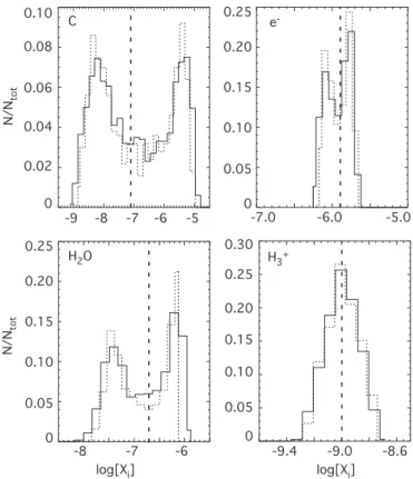
Fig. 2. Distributions (nomalized to the total number of runs) of
the abundances of C, H2O, e− and H+3 at 107 yr (high-metal
case). The solid lines refer to the variation of all the rate coef-ficients whereas the dotted lines represent the variation of ζHe
and ζH2only. The vertical dashed line represents the abundance
computed with the standard values of the rate coefficients.
tions are obtained for a large number of species (C, H2O, SO,
CS etc) with the largest separation between the two peaks for atomic carbon (three orders of magnitude). Fig. 2 shows his-tograms for the abundance distributions of the species C, H2O,
e−, and H+
3 at 10
7 yr. It can be seen that the H+
3 distribution
does not show a bimodal profile but is Gaussian. The same is true for H2S and OH. Since the error in the rate coefficients
fol--16.8 -17.2 -17.0 0 log(k[cm-3]) 0.2 0.4 0.6 0.8 1.0 0.0 -16.8 -17.2 -17.0 100 200 300 -17.4 -17.2 -17.0 0 log(k[cm-3]) 0.2 0.4 0.6 0.8 1.0 0.0 -17.4 -17.2 -17.0 N u mbe r of ru n s 100 150 200 250 300 50 0 log(k[cm-3]) -7.20 -7.15 -7.10 -7.05 0.2 0.4 0.6 0.8 1.0 0.0 100 200 300 -7.20 -7.15 -7.10 -7.05 ζHe He + CRP He+ + e- ζH2 H2 + CRP H2+ + e- H3+ + e- H2 + H h is t 2 / h is t 1 hist 1 hist 2
Fig. 3. Histograms of the rate coefficients of the following
reac-tions (upper panel): He + CRP → He++ e−(ζHe, left box), H2 + CRP → H+
2 + e
−(ζ
H2, middle box) and H
+
3 + e
−→H
2+ H
(right box). The thick and thin lines represent the histograms of all the runs (hist 1) and of the runs giving the higher abundance of O2(hist 2, see text) respectively. The lower panels show the
ratio between hist 2 and hist 1.
lows a log-normal distribution, the bimodal shapes are due to non-linear effects.
We obtained the bimodal distributions by varying the rate coefficients, we then decided to identify the reactions responsi-ble for them if at all possiresponsi-ble. We proceeded as follows. Among the 2000 runs, we listed the sets of reactions that give one the higher of the two most probable abundances for O2. Then for
each rate coefficient, we plotted the histograms for all runs and the histograms for those runs giving only the higher abundance of O2. In the upper panels of Fig. 3, pairs of histograms can be
seen for the rate coefficient of the cosmic ray ionization of He, that of H2, and the dissociative recombination of H+3 to form H2
and H. The thick lines (hist1) represent histograms for all runs while the thin lines (hist2) represent those ending up with the higher O2abundance. For reactions not responsible for the
bi-modal distributions, there should be no difference between the pairs of histograms except that the total number of runs should be lower for the second one. For most of the reactions, we in-deed found no difference, as for the reaction H+
3 + e
−→H
2+
H in Fig. 3. In fact, there were only two exceptions: the direct ionization rate coefficients of He and H2 by cosmic rays (ζHe
and ζH2), and their marked effect can be seen in Fig. 3. The
high abundance of O2tends to be formed with lower values of ζHeand higher values of ζH2, as can be seen most clearly in the
lower panels of Fig. 3, in which the ratios of the two histograms are plotted. It is then convenient to consider the sensitivity of the abundance of O2and other species to the ratio ζHe/ζH2rather
than to their absolute values. To confirm their importance, we randomly varied only ζHeand ζH2, keeping the other rate
coeffi-cients constant, and we obtained the same bimodal distribution as with the fully random method at steady state. The dispersion of the abundances in this case is then almost as large as when we varied all the rate coefficients, as can be seen in the dotted lines in Fig. 2.
The sensitivity of the chemical abundances to the ratio
ζHe/ζH2can be explored in another way. In Fig. 4 (left panel),
ran-4 V. Wakelam et al.: Extreme sensitivity of the dense cloud chemistry 0.1 1.0 10.0 lo g( Xi ) O2 -8 -7 -6 -5 -4
Variation of all the rate coefficients ζHe sampling 0.1 1.0 10.0 -8 -7 -6 -5 -4 ζHe/ζH2 ζH2 sampling lo g( Xi ) 0.1 1.0 10.0 -8 -7 -6 -5 -4 Variation of ζHe and ζH2 only lo g( Xi )
Fig. 4. Abundance of O2as a function of ζHe/ζH2at 10
7yr. The
upper and middle panels represent the abundance computed with the random distribution of all the rate coefficients and of
ζHeand ζH2only, respectively. The solid lines in the lower plot
have been computed using one value of ζHe for each line and
varying ζH2 , while the dotted lines have been computed
us-ing one value of ζH2for each line and varying ζHe. The vertical
dashed line indicates the standard value of ζ0 He/ζ
0 H2.
domly varying all the rate coefficients as a function of ζHe/ζH2.
For comparison, the abundance computed with the random variation of ζHeand ζH2only is shown in the middle plot of the
figure. The smaller vertical dispersion is caused by not varying the other rate coefficients. Finally and for more clarity, we de-pict, in the lower panel, the calculated O2abundance as a
func-tion of ζHe/ζH2obtained by calculations in which the ionization
rates are not varied randomly. Rather, the solid lines show val-ues of the steady-state O2abundance computed for 5 values of ζHe(between 2ζHe0 and ζHe0 /2) with ζH2varied to account for the
range of the abscissa between 0.05 and 5. In the same panel, dotted lines show the O2abundances computed for 5 values of ζH2with ζHevaried to account for the range of the abscissa. The
abundances computed by each method are similar especially at
ζHe/ζH2 H3+ -10.0 0.1 1.0 10.0 -9.5 -9.0 -8.5 -8.0 H2O -8.0 0.1 1.0 10.0 -7.5 -7.0 -6.5 log (Xi ) log (X i ) 0.1 1.0 10.0 -5 e --6 -7 -8 -9 -5.7 -5.8 -5.9 -6.0 -6.1 -6.2 0.1 1.0 10.0 C ζHe/ζH2
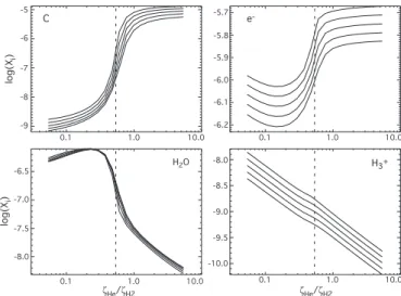
Fig. 5. Abundances of C, e−, H2O and H+3 as a function of ζHe/ζH2 and for five different values of ζHe (solid lines). The
vertical dashed line indicates the standard value of ζ0 He/ζ
0 H2.
the inflection point, confiming that the choice of the ionization ratio as a parameter of the sensitivity is a reasonable one.
The abundance of O2 decreases by two orders of
magni-tude (from 10−5 to 10−7) when ζ
He/ζH2 goes from 0.3 to 0.8,
and the inflection point of the curve occurs at the standard value of ζ0
He/ζ 0
H2used in osu.2003 (0.5/0.93). In Fig. 5 we show
some other examples of this sensitivity by using five differ-ent values of ζHe, as in the solid lines of the right panel of
Fig. 4. The abundance of atomic carbon has an almost equal sensitivity albeit opposite to that of O2, while the H2O
abun-dance shows a similar profile to O2 except for a local
maxi-mum at ζHe/ζH2around 0.2. Although the electronic abundance
increases towards higher ζHe/ζH2, it varies only a factor of 2.5
between ζHe/ζH2=0.1 and ζHe/ζH2=3. The abundance of the H
+
3
ion, which does not show any bimodal distribution, is linear with ζHe/ζH2. The dispersion of the abundances, for a given
ra-tio ζHe/ζH2, due to the variation of ζHeby a factor of 2 around
the standard value ζ0
He, depends on the species: it is smaller for
H2O, O2 and e−than for C and H+3, for instance, but remains
anyway below 0.5 dex.
4. Sensitivity for different model parameters
4.1. Other choices of elemental abundances
The calculated sensitivity depends on the elemental abun-dances used for the modeling. In Fig. 6, we show the C, H2O,
e− and H+
3 fractional abundances as a function of ζHe/ζH2 for
the low-, intermediate-, and high-metal elemental abundances (see Sect. 2). The sensitivity plots, as well as most others later in the paper, are obtained by fixing the helium ionization rate at its standard value so that no dispersion is seen. The H2
den-sity remains at 104cm−3and the temperature at 10 K. Although
the sensitivity exists for the three cases, the inflection point is shifted to higher values of ζHe/ζH2 for the low-metal case. For
the intermediate case, on the other hand, the sensitivity seems to be stronger, leading to an abrupt jump in the abundance of
log (Xi ) -5 -6 -7 -8 -9 C 0.1 1.0 10.0 -10 e -0.1 1.0 10.0 -5 -6 -7 -8 ζHe/ζH2 0.1 1.0 10.0 H2O log (Xi ) -6 -7 -8 -9 0.1 1.0 10.0 H3+ ζHe/ζH2 -7 -8 -9 -10 high metal inter. metal low metal
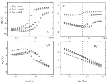
Fig. 6. Steady-state abundances of C, e−, H
2O and H+3 as
functions of ζHe/ζH2 for three different elemental abundances.
The triangles, diamonds and crosses represent the low-, intermediate-, and high-metal cases. The vertical dashed line indicates the standard value of ζHe0 /ζH0
2. The H2 density is
104cm−3and the temperature 10 K. The value of ζHeis fixed at
its standard value while ζH2is varied.
-8 -7 -6 -9 -5 log[Xi] 0 0.05 0.10 0.15 0.20 0.25 0.30 -8 -7 -6 -9 -5 log[Xi] 0 0.05 0.10 0.15 0.20 0.25 0.30 -8 -7 -6 -9 -5 log[Xi] C N / Nto t 0 0.05 0.10 0.15 0.20 0.25 0.30
Low metal Intermediate metal High metal
Fig. 7. Distribution (nomalized with respect to the total number
of runs) of the steady-state abundance of atomic carbon for the three sets of elemental abundances. The vertical dashed line represents the abundance computed with the standard values of the rate coefficients.
C for ζHe/ζH2=1.1. A similar abrupt change can be seen for the
electronic abundance. This jump is actually a manifestation of bistability (see section 5). Note that for ζHe/ζH2<1.1, the
abun-dances for the intermediate-metal case tend to be close to the low-metal ones whereas for ζHe/ζH2 > 1.1 they are similar to
the high-metal ones.
When one runs the uncertainty method with a factor of two uncertainty in ζHe and ζH2, the values of ζHe/ζH2 are spread
approximatively between 0.13 and 2.2. The distribution of the abundances computed with this method thus depends on the sensitivity within this range of values. The distribution of the steady-state abundances of C computed by variation of all the rate coefficients are shown in Fig. 7 for the three sets of abundances. Because the inflection point for the low-metal case is shifted to ζHe/ζH2=2, the uncertainty method gives
0.1 1.0 10.0 ζHe/ζH2 -6 -7 -8 -9 -10 -11 High Metal -5 0.1 1.0 10.0 ζHe/ζH2 -6 -7 -8 -9 -10 -11 Intermediate Metal -5 0.1 1.0 10.0 ζHe/ζH2 -6 -7 -8 -9 -10 -11 log( Xi ) C/O=0.2 C/O=0.4 C/O=0.6 Low Metal -5
Fig. 8. Atomic carbon abundance at steady state as a function of ζHe/ζH2for the three elemental abundances (low-,
intermediate-, and high-metal). In each plotintermediate-, the symbols refer to different C/O ratios. The vertical dashed line indicates the standard value of ζHe0 /ζH0
2.
Gaussian-like distributions although slightly asymmetrical to-wards higher C abundances. This explains why we did not see the sensitivity effect in our previous work on rate coefficient uncertainties in dark clouds (see Wakelam et al. 2006). For high-metal elemental abundances, the point of inflection occurs close to the standard value of ζHe/ζH2=0.54 and the distribution
for the C abundance is bimodal. When using the intermediate-metal abundances, the uncertainty method gives two distinct peaks with no solutions between them. The peak at higher abundance is the smaller since the point of inflection occurs at values of ζHe/ζH2=1.1 somewhat larger than the standard.
The lack of any model runs with steady-state abundances in between the two distributions stems from the sharpness of the curve around the inflection point and is a consequence of the bistability.
In addition to its dependence on metallicity, the sensitivity to ζHe/ζH2 depends strongly on the C/O elemental abundance
ratio. In Fig. 8, we show the steady-state abundance of atomic carbon as a function of ζHe/ζH2 computed for the three sets of
elemental abundances, each with three different values of C/O – 0.2, 0.4 (the standard one), and 0.6 – obtained by maintain-ing a constant carbon abundance while varymaintain-ing the oxygen. The lower the C/O ratio is, the more the inflection point is shifted towards higher values of ζHe/ζH2. As an example, the inflection
point for the high-metal case occurs around 0.2 for C/O=0.6 whereas it rises to 1.5 for C/O=0.2. In both cases, the inflection point is too far from the standard value of ζHe/ζH2 to obtain a
bimodal distribution. For the intermediate-metal case, the C/O ratio of 0.6 results in shifting the inflection point to the stan-dard value of ζHe/ζH2, so that the analogous panel to the one in
Fig. 7 would show two equal areas for the two peaks. The dis-persion of the carbon abundance caused by the variation of C/O is larger for values of ζHe/ζH2 smaller than the inflection point
while the abundances eventually form a single plateau after the jump.
As discussed in Wakelam & Herbst (in preparation), the helium abundance used in the classic low- and high-metal el-emental abundances (see Section 2) is quite high (0.28 com-pared with H2) compared with the more modern value of 0.18
measured in the interstellar medium (see, for example, Baldwin et al. 1991). Naturally, the sensitivity will change if a lower value of He is used. Fig. 9 shows the distribution of the steady-state C abundance computed with a random variation of ζHeand ζH2 and the high-metal case with the lower helium abundance.
6 V. Wakelam et al.: Extreme sensitivity of the dense cloud chemistry C 0 0.05 0.10 0.15 N / Ntot -8 -7 -6 -9 -5 log[Xi] 0.20 C -5 -6 -7 -8 -9 0.1 1.0 10.0 -10 ζHe/ζH2 high metal inter. metal low metal log[ Xi ]
Fig. 9. The left panel shows the distribution of the steady-state
abundance of atomic carbon computed with a random variation of ζHeand ζH2for the high-metal elemental abundances but with
a lower helium elemental abundance of 0.18 compared with H2. The right panel represents the C steady-state abundance as
a function of ζHe/ζH2 for the three elemental abundances with
the low He abundance. The vertical dashed line indicates the C abundances computed with the standard ζ0
Heand ζ 0
H2on the left
plot and the standard value of ζHe0 /ζH0
2on the right plot.
ζHe/ζH2 0.1 1.0 10.0 log( Xi ) -4 -5 -6 -7 -8 -9 High Metal Low Metal Srates -10 -4.0 -5.0 -6.0 -7.0 -4.5 -5.5 -6.5 -7.5 ζHe/ζH2 0.1 1.0 10.0 High Metal Low Metal rate99
Fig. 10. Abundance of C as a function of ζHe/ζH2computed with
the high- (black lines) and low- (grey lines) metal abundances. The left and right panels show the results using the Srates (see text) and rate99 networks. The vertical dashed line indicates the standard value ζ0
He/ζ 0 H2.
In this case, we do not obtain a clear bimodal distribution but merely an asymmetrical profile, because the inflection point is shifted towards higher values of ζHe/ζH2, as shown in Fig. 9,
and the random method barely reaches the sensitive portion of the curve.
4.2. Chemical database
To test the influence of the chemical network utilized, we con-structed the sensitivity curves at steady-state with two other databases – Srates and rate99– using both low-metal and high-metal abundances. The rate99 network is the UMIST list of reactions (Le Teuff et al. 2000) prior to its current updating (see http://www.udfa.net) whereas Srates is the list of reactions used by Wakelam et al. (2004) to study sulphur chemistry in hot cores. This latter network contains only five elements (H, He, C, O and S) but, as discussed in Wakelam et al. (2004), the steady-state abundances computed with it are very close to the ones computed with the larger osu.2003 network at low
tem-ζHe/ζH2 nH2 log (X i )
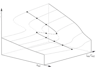
Fig. 11. Illustrative scheme of hysteresis surface
demonstrat-ing bistability with two “orthogonal” control parameters, here nH2and ζHe/ζH2). The position of unstable solutions is indicated
by dashed lines . Orthogonal cuts crossing the folding region produce hysteresis curves like the ones shown in Fig. 12 and Fig. 13.
perature. The ionization rates for H2and He are the same in all
three databases.
Fig. 10 is a sensitivity plot of the C abundance for five dif-ferent values of ζHe between 2ζHe and ζHe/2. The sensitivity
obtained with Srates is similar to that for osu.2003, which indi-cates that the absence of the other elements (Si, Fe, Na etc.) does not change the sensitivity drastically. On the contrary, the results with rate99 show a much different relation between
ζHe/ζH2 and the atomic carbon abundance, especially for the
high-metal case, where the rate99 curves show (a) a signifi-cantly lower value for the point of inflection of the sensitivity, (b) a wide dispersion due to the value of ζHeat low values of ζHe/ζH2, and (c) a much smaller jump in the abundance. We
have shown in Wakelam et al. (2006) that rate99 and osu.2003 often have differences in rate coefficients larger than the esti-mated random errors for unstudied reactions of a factor of 2, whereas most of the rate coefficients in Srates are taken from the osu database. Since the three networks have the same ζHe
and ζH2, the shape of the sensitivity can depend only on the
values of other rate coefficients.
5. Bistability
In section 4, we saw that the variation of ζHe/ζH2leads to a sharp
change in the abundances of some species for the intermediate-metal case (see Fig. 6). This jump is indeed a manifestation of the same bistability discovered by Le Bourlot et al. (1993), as can be determined by comparing the region of the bistability in parameter space. The parameter usually used to study this bistability is the ratio between the cosmic-ray ionization rate ζ and the density nHbut other model parameters such as the
tem-perature and rate coefficients have been used (Le Bourlot et al. 1995; Pineau Des Forˆets & Roueff 2000). What we have found here is that ζHe/ζH2 is also a control parameter which explore
0.1 1.0 10.0 lo g( Xi ) -12 -10 -8 -6 -4 ζHe/ζH2 0.1 1.0 10.0 lo g( Xi ) -12 -10 -8 -6 -4 -12 -10 -8 -6 -4 0.1 1.0 10.0 ζHe/ζH2 0.9 1.0 0.8 -9 -8 -7 -6 -5 log (Xi )
Low Metal High Metal
Intermediate Metal ζHe/ζH2 ζHe/ζH2 106cm-3 105cm-3 104cm-3 103cm-3 102cm-3 106cm-3 105cm-3 104cm-3 103cm-3 102cm-3 106cm-3 105cm-3 104cm-3 103cm-3 102cm-3 104cm-3
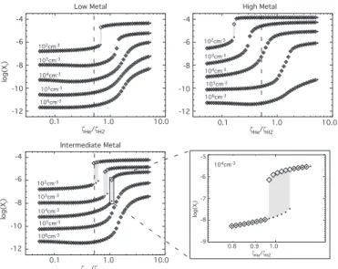
Fig. 12. Hysteresis curves of the steady-state abundance of
atomic carbon as a function of ζHe/ζH2 for three different
ele-mental abundances (low-, high-, and intermediate-metal), and for five H2 densities between 102and 106 cm−3. The vertical
dashed line indicates the standard value of ζHe0 /ζH0
2. Grey zones
indicate regions of bistability.
-5 -6 -7 -8 -9 0.1 1.0 10 ζHe/ζH2 e -nH2 (cm-3) 101 102 103 104 105 lo g (X i ) -5 -6 -7 -8 -9 e -102 103 104 105 106 cm-3 ζHe0/ζH20
Fig. 13. Hysteresis curves of the electron steady-state
abun-dance as a function of nH2(left panel) and ζHe/ζH2(right panel).
Intermediate-metal elemental abundances are used for both plots. Five H2densities between 102and 106cm−3are used for
the right panel. The vertical dashed line indicates the standard value of ζ0
He/ζ 0
H2. Grey zones indicate regions of bistability.
be an orthogonal axis to ζ/nH, the bistability of Le Bourlot et al.
(1993) is the same as ours when ζHe/ζH2is at its standard value.
In Fig. 11, we show an illustrative scheme of this bistability as controlled by the two parameters nH2and ζHe/ζH2. To make the
bistability appear, we constructed hysteresis curves as a func-tion of ζHe/ζH2for different H2 densities. These curves, shown
in Fig. 12 for atomic carbon, were produced in two steps. Fist, we ran the model to compute the steady-state abundance us-ing one value of ζHe/ζH2, then we used this solution as the
ini-tial condition and increased ζHe/ζH2 to compute the next point,
shown as the crosses in Fig. 12 and 13. In addition, the same principle but with decreasing ζHe/ζH2was utilized, with results
shown as diamonds.. In order to vary ζHe/ζH2, we fixed the
he-lium ionization rate and changed that of hydrogen. When two
solutions exist for a range of ζHe/ζH2values, a region of
bista-bility exists.
To explore the domains of bistability using the new control parameter, we constructed hysteresis curves using the three dif-ferent elemental abundances and five densities between 102and 106 cm−3. All the results are shown in Fig. 12 for atomic
car-bon. Bistability exists for all the elemental abundances but the domain of ζHe/ζH2where the two solutions coexist are small. To
show the bistability more clearly, a magnification of this region is done for n(H2)=104cm−3 and the intermediate-metal case.
In both the low- and high-metal cases, bistability exists only at very low density (102 cm−3) whereas in the
intermediate-metal case, the bistability exists between 102 and 104 cm−3.
The increase in density shifts and smoothes the inflection point, making the bistability eventually disappear. Note that this is the first time that the bistability has been found with the high-metal case (Lee et al. 1998; Boger & Sternberg 2006), because it does not exist for the standard value of ζHe/ζH2. We have
con-firmed that, for the high-metal case, using the standard value of ζHe/ζH2 leads to no bistability with nH2 as low as 10 cm
−3.
Using ζHe/ζH2= 0.16 however, bistability exists in a very small
density range of 70-90 cm−3.
A more focused look at the two control parameters is shown in Fig. 13, where we plot the hysteresis curves of the elec-tron abundance as a function of each parameter for the case of intermediate-metal elemental abundances. The value of ζ is set at the standard value. For the variation of ζHe/ζH2 (right
panel), we used five H2 densities between 102and 106 cm−3,
as in the previous figure, while for the hysteresis curve as a function of nH2 (left panel) the standard value of ζHe/ζH2
(0.54) was used and the bistability found to exist in the density range 60-150 cm−3. With the other control parameter and for
nH2 = 10
2cm−3, the bistability exists for ζ
He/ζH2between 0.5
and 0.7 and the domains of bistability using both parameters overlap. For higher densities, the bistable region using ζHe/ζH2
shifts towards higher values and so does not exist anymore in the hysteresis curve versus nH2. These hysteresis curves can be
combined into a plot of the type shown in Fig. 11.
6. Chemical reactions involved in the sensitivity
The sensitivity of the abundances to the ratio ζHe/ζH2 is
re-lated to the non-linearity of the system. A detailed mathemat-ical analysis of this phenomenon is in progress (Massacrier et al., in preparation). It is possible, however, to understand the difference, between the low and high ζHe/ζH2 phases
qualita-tively from a chemical point of view. For this purpose, we have considered the main reactions of production and destruction of O, C, CO, S and SO, which are the main reservoirs of car-bon, oxygen and sulphur for the intermediate- and low-metal elemental compositions in which sulfur is relatively abundant, and/or are the species most influenced by ζHeand ζH2. Let us
first consider low values of ζHe/ζH2. The ionization of H2leads
to the formation of OH through a well-known series of reac-tions (see. e.g. Boger & Sternberg 2006). The radical OH then reacts with atomic oxygen to form O2. The most efficient way
of destroying O2is to form SO by reaction with S. Since the
8 V. Wakelam et al.: Extreme sensitivity of the dense cloud chemistry
oxygen, large amounts of O2remain in the gas phase. Atomic
carbon reacts with O2to form CO where it is stored since CO
is not efficiently destroyed. For high ζHe/ζH2, on the other hand,
the destruction of CO by He+ produces C+and O more
effi-ciently. Carbon ion then exchanges its charge with S so large abundances of C remain in the gas phase to deplete molecular oxygen.
Since the bistability we see is an extreme manifestation of the sensitivity to ζHe/ζH2, the chemical processes involved in
bistability may be related to those discussed above, although our control parameter is different from those previously stud-ied. Pineau des Forets et al. (1992) and Le Bourlot et al. (1993, 1995) identified the abundance ratio H+/H+
3 as being
impor-tant for bistability, with one ion identified with the HIP and the other with the LIP solution. The abundance ratio H+/H+3
depends on the abundance of electrons and as a consequence on the efficiency of the dissociative recombination of H+3 with electrons, the rate of which was quite uncertain at the time. In our analysis however, the H+3 ion shows little if any sensitivity to the control parameter, although the electron abundance does show a jump between the low and high ζHe/ζH2 phases, which
can then be thought of as analogous in some sense to the LIP and HIP solutions. Recently, Boger & Sternberg (2006) made another detailed analysis of the chemical differences between the so-called HIP and LIP solutions, arguing that bistability is due to a loop including H+
3, O2 and S
+. Although this expla-nation is related in some aspects to that given for the sensitiv-ity reported here, one must remember that our control parame-ter raises some new points, given the relation of the ionization rate of He to the formation of the important ion C+, which is a precursor for many species, and can charge exchange to form abundant C. Moreover, S+, which is prominent in the explana-tion of Boger & Sternberg (2006), is not the dominant charge carrier in our calculations. Note that the osu.2003 database in-cludes the recombination of the main ions with negative grains and this does not cancel the bistability, although such a cancel-lation was suggested by Boger & Sternberg (2006). It may well be that the H+/H+
3 abundance ratio, the H
+
3-O2-S
+cycle, and the ζHe/ζH2ratio comprise pieces of a larger and more complex
jigsaw puzzle. Since bistability also appears to be a function of the reaction network utilized, secondary reactions may play a more important role than heretofore realized. This possibility has to be clarified through the building of a simplified reaction network that still shows the main characteristics of bistability.
7. Observational relevance
The sensitivity to ζHe/ζH2depends highly on the model
param-eters and, for this reason, it is not obvious if such effect can be detected in the interstellar medium. In an ideal situation where the cloud characteristics (at least the elemental abundances and the age) are well known and correspond to a distinct chemical regime, one could use the observations to constrain the ratio
ζHe/ζH2assuming however that no local variation of this ratio is
expected. In reality, the cloud characteristics are in general far from being well constrained, and an analysis of the uncertain-ties in the ionization rates of H2and He is strongly required to
understand the relevance of this sensitivity for the interstellar
medium. Note that ζHe/ζH2is not sensitive to the total intensity
of the cosmic-ray flux.
If the intermediate-metal elemental abundances reflect the cloud characteristics and if the ionization rate of He and H2by
cosmic-rays can vary by at least a factor of 2 within a cloud, the prediction of bistability over a wide range of densities sug-gests that strong chemical heterogeneities in dense clouds can be caused by this effect. In the absence of bistability an ex-treme sensitivity is predicted at most densities for low-metal and high-metal abundances and may cause some observed het-erogeneities in abundance. However, we have to consider the age of the cloud. The bifurcation occurs just after 105yr,
start-ing from our standard initial conditions, and is a maximum at steady-state (> 107yr). As a consequence, the chemical hetero-geneity can be caused by this sensitivity only in evolved clouds (> 105−106yr).
The large gas-phase abundances of H2O and O2molecules
predicted by dense cloud chemical models is a long standing problem. Using high values of ζHe/ζH2, we obtain much smaller
abundances for these species, closer to the upper limits in dense clouds (Bergin & Snell 2002; Pagani et al. 2003). Large uncer-tainties in the ζHe/ζH2 ratio could then solve the problem
re-lated to the modeling of water and molecular oxygen. One has, however, to consider the overall picture, and the better agree-ment with H2O and O2should not worsen the agreement for the
other species. A comparison between observations and model-ing should be done in a systematic way, as done by Wakelam et al. (2006). This was not the purpose of the present study, but we can already note, as an example, that the observed abun-dances in L134N (North peak) of OH and C4H (7.5 × 10⁻⁸and
10−9 respectively, Ohishi et al. 1992) are reproduced by the
model when using the standard value of ζHe/ζH2 but are
under-estimated when using the higher ratios ζHe/ζH2 that reproduce
H2O and O2abundances.
Finally, the very low H2 density (100 cm−3), at which the
bistability as a function of ζHe/ζH2is restricted to with the
low-and high-metal elemental abundances, is not relevant for clouds with the assumed visual extinction (Av=10) since it would
re-quire a size of 26 pc, which is much larger than typical cloud sizes (Snell 1981).
8. Conclusions
Using a Monte Carlo uncertainty method to compute the theo-retical error of molecular abundances in chemical models, we found a strong sensitivity of the steady-state abundances to the ratio between the ionization rate coefficient of helium ζHeand
that of molecular hydrogen ζH2by cosmic rays. This sensitivity
to the ratio has the consequence of changing the abundance of some species by several orders of magnitude for small varia-tions of ζHe/ζH2. Lower values of ζHe/ζH2 are characterized by
large abundances of smaller molecules such as O2, H2O, SO,
etc. whereas high values of ζHe/ζH2 lead to large abundances
of atoms. If the sensitivity is strong enough, it can result in the phenomenon of bistability, which we located at low densi-ties for two sets of elemental abundances - the low- and high-metal cases, and over a wide range of densities for the case of the so-called intermediate-metal abundances, in which
sul-fur plays a particularly prominent role. The bistability has been determined to be the same as studied earlier by a variety of au-thors with other control parameters; it is perhaps simplest to consider our control parameter – ζHe/ζH2– as orthogonal to one
of the others - the ratio of the overall ionization rate parameter
ζ to the density n – so that the bistability can be imagined to exist in a region in three-dimensional space rather than in the customary two-dimensional hysteresis picture.
It is interesting to speculate that the sensitivity detected here via our uncertainty analysis is a necessary but not suffi-cient condition for bistability because only the most extreme sensitivity, in which the bimodal distributions detected have no solutions in between them, leads to bistability. Unfortunately, it is not guaranteed that our type of uncertainty analysis can always locate a bistable region since finding an extreme sensi-tivity may require large uncertainties in some parameters, such as the gas density, to take us from our standard parametric val-ues to the bistable region.
Several questions arise when considering the dramatic ef-fects of small ζHe/ζH2 variations on the gas-phase chemistry.
First, even if one assumes a given flux and energy distribution of the cosmic rays, the determination of ζHe/ζH2 suffers some
significant uncertainties, with the role of secondary electrons particularly important. Besides these difficulties, one might also have to consider variations of the ratio ζHe/ζH2 in space,
such as between one cloud and another, or between the cen-ter and the edges of a same cloud, and in time. Changes in the ratio imply important variations in the spectral distribution of the cosmic rays (Glassgold & Langer 1973). Such variations might be produced by the attenuation of the cosmic rays inside a cloud or the proximity of supernovae in star forming clouds. Whether such variations are expected or not and how they could affect the chemistry should be considered in the future. Finally, a knowledge of the helium elemental abundance appears to be crucial since the sensitivity region depends on this parameter.
Acknowledgements. V. W. and E. H. thank the National Science
Foundation for its partial support of this work. G.M. acknowledges partial financial support from the CNRS/INSU programs PCMI and PNPS.
References
Baldwin, J. A., Ferland, G. J., Martin, P. G., et al. 1991, ApJ, 374, 580
Bergin, E. A. & Snell, R. L. 2002, ApJ, 581, L105 Black, J. H. 1975, Ph.D. Thesis
Boger, G. I. & Sternberg, A. 2006, ApJ, 645, 314 Charnley, S. B. & Markwick, A. J. 2003, A&A, 399, 583 Dalgarno, A., Yan, M., & Liu, W. 1999, ApJS, 125, 237 Glassgold, A. E. & Langer, W. D. 1973, ApJ, 186, 859 Graedel, T. E., Langer, W. D., & Frerking, M. A. 1982, ApJS,
48, 321
Herbst, E. & Klemperer, W. 1973, ApJ, 185, 505
Le Bourlot, J., Pineau des Forets, G., & Roueff, E. 1995, A&A, 297, 251
Le Bourlot, J., Pineau des Forˆets, G., Roueff, E., & Schilke, P. 1993, ApJ Lett., 416, L87+
Le Teuff, Y. H., Millar, T. J., & Markwick, A. J. 2000, A&AS, 146, 157
Lee, H.-H., Roueff, E., Pineau des Forˆets, G., et al. 1998, A&A, 334, 1047
Ohishi, M., Irvine, W. M., & Kaifu, N. 1992, in IAU Symp. 150: Astrochemistry of Cosmic Phenomena, Vol. 150, 171 Pagani, L., Olofsson, A. O. H., Bergman, P., et al. 2003, A&A,
402, L77
Pineau Des Forˆets, G. & Roueff, E. 2000, in Astronomy, physics and chemistry of H+
3, 2549–+
Pineau des Forets, G., Roueff, E., & Flower, D. R. 1992, MNRAS, 258, 45P
Shalabiea, O. M. & Greenberg, J. M. 1995, A&A, 296, 779 Smith, I. W. M., Herbst, E., & Chang, Q. 2004, MNRAS, 350,
323
Snell, R. L. 1981, ApJS, 45, 121
Terzieva, R. & Herbst, E. 1998, ApJ, 501, 207
Wakelam, V., Caselli, P., Ceccarelli, C., Herbst, E., & Castets, A. 2004, A&A, 422, 159
Wakelam, V., Herbst, E., & Selsis, F. 2006, A&A, 451, 551 Wakelam, V., Selsis, F., Herbst, E., & Caselli, P. 2005, A&A,