HAL Id: hal-02191385
https://hal-lara.archives-ouvertes.fr/hal-02191385
Submitted on 23 Jul 2019
HAL is a multi-disciplinary open access
archive for the deposit and dissemination of
sci-entific research documents, whether they are
pub-lished or not. The documents may come from
teaching and research institutions in France or
abroad, or from public or private research centers.
L’archive ouverte pluridisciplinaire HAL, est
destinée au dépôt et à la diffusion de documents
scientifiques de niveau recherche, publiés ou non,
émanant des établissements d’enseignement et de
recherche français ou étrangers, des laboratoires
publics ou privés.
Thermal and field-aligned drift effects of the potential
created by an alterning point charge in a
magnetoplasma near the lower oblique resonance
J. Thiel
To cite this version:
J. Thiel. Thermal and field-aligned drift effects of the potential created by an alterning point charge
in a magnetoplasma near the lower oblique resonance. [Research Report] Note technique CRPE n°
40, Centre de recherches en physique de l’environnement terrestre et planétaire (CRPE). 1977, 59 p.
�hal-02191385�
CENTRE NATIONAL D'ETUDES DES TELECOMMUNICATIONS
CENTRE NATIONAL DE
LA RECHERCHE SCIENTIFIQUE
CENTRE DE RECHERCHE EN PHYSIQUE DE
L'ENVIRONNEMENT TERRESTRE ET PLANETAIRE
NOTE TECHNIQUE CRPE/40
THERMAL AND FIELD-ALIGNED-DRIFT EFFECTS ON THE POTENTIAL CREATED BY
AN ALTERNATING POINT CHARGE IN A MAGNETOPLASMA NEAR THE LOWER OBLIQUE RESONANCE
par
J. THIEL
C.R.P.E./P.C.E.
45045 - ORLEANS CEDEX
Le Chef du Département P.C.E.
P. Le Directeur
J. HIEBLOT C. BEGHIN
CONTENTS
Abstract 3
I. Introduction 4
II. General theory for a drifting Maxwellian magnetoplasma... 7
III. Thermal effects in a stationary Maxwellian magnetoplasma... 12
IV. Drift effects in a cold magnetoplasma... 18
V. Combined effects of thermal and drift motions... 27
VI. Summary and conclusions... 35
Acknowledgements... 39
Footnotes... 40
- 3 -
ABSTRACT
A rapid method is used to find the least-damped root of the dispersion équation for electrostatic waves in a Maxwellian magnetoplasma, including the effects of field-aligned drift ; the low température and low-drift-speed approximations are avoided. Calculations are made of the potential created by an alternating point charge at a frequency
less than both the plasma and the électron cyclotron frequencies, neglec- ting collisions, forced ion motion, and the contributions of higher-order roots. A comparison of the numerical results with the approximate expres- sions previously published shows that the latter are inadéquate for dia- gnostic purposes, i.e. for deducing électron density, température, and drift velocity from measurements of the potential.
I. INTRODUCTION
Récent experiments in the laboratoryl-4 and in spaceS-7 hâve confirmed the existence of the so-called cône or oblique résonances of a magnetoplasma in certain frequency bands. If the forced motion of the positive ions is neglected, there are only two such bands : the upper band extends from the upper hybrid frequency down to either the plasma frequency or the électron cyclotron frequency, whichever is the higher ; the lower band extends from the lower of thèse two frequencies downwards. The présent paper is concerned exclusively with the résonance in this lower band, hereinafter referred to as the lower oblique résonance.
In a stationary magnetoplasma, the scalar potential set up by a small monopole antenna has rotational symmetry around the magnetic field line that passes through the antenna and reflexion symmetry with respect to a plane that includes the antenna and is perpendicular to the field lines. Thus, if this antenna is excited with a sinusoidal current of fixed amplitude and frequency, the alternating potential received on a second monopole, at a vector distance r from the first, dépends only on the magnitude r of this distance and on the angle 3 between r and the magnetic field direction. Now, in the above frequency bands, if the angle 3 is varied in the range 0 - IT/2 while r is kept constant, the amplitude of the received potential exhibits quasi-sinusoidal variations ; the alternate maxima and minima correspond to an interférence structure. The highest maximum occurs at a certain angle 3
which is that of the so-called résonance cône. The secondary maxima occur only on one side of this cône ; they are regularly speced, and decrease steadily Ln amplitude as 18 - 3 increases. Because both the résonance cône angle and the spacing of the secondary maxima dépend on the électron density and température, it has been suggested that thèse two parameters could be determined from measurements of the angular variation of the potential.
- 5 -
When the plasma is drifting along the magnetic field, the
rotational symmetry of the scalar potential is unaffected but the reflexion symmetry is destroyed : the résonance cône becomes wider upstream and narrower downstream. This angular shift has not yet been detected experi- mentally, however. Usually it is easier to make précise measurements of
frequency rather than of angle, so the suggestion has been made that it would be more fruitful to look for the corresponding shift in résonance
frequency at a fixed angle8. The sign of the frequency shift dépends upon which antenna is transmitting and which is receiving : the shift
is towards lower frequencies when the receiver is upstream from the trans- mitter, and conversely. Measurements of this non-reciprocal effect could be used to détermine the électron drift velocity parallel to the magnetic
field and hence the field-aligned électron current.
Thermal effects on the angular variations of the potential and of the field created by an alternating point charge in a homogeneous sta- tionary magnetoplasma hâve already been investigated theoretically, assu- ming a Maxwellian électron distribution function. Neglecting collisions and forced ion motion, Fisher and Gould and Singh and Gould derived thèse variation analytically - and calculated their numerically - in the limit of an infinité magnetic field. Later, Kuehl11'12, Chasseriaux and Burrell1* extended their calculation to the case in which the magnetic field is finite but they used the low-temperature approximation among others, which drastically simplify the dispersion équation for electrostatic waves : there is only one root, and its damping is neglected. In the présent paper, we report numerical calculations of the potential made neglecting collisions and forced ion motion, using the exact dispersion équation, but retaining only the least-damped root, which corresponds to that given by the low-temperature approximation.
The effects of field-aligned drift on the frequency variation of the coupling impédance between two monopoles in a cold homogeneous magnetoplasma hâve been studied by Storey and Pottelette11* ' ] 5 . They neglected collisions and forced ion motion and assumed that the électron plasma frequency was much higher than the cyclotron frequency. Moreover, they considered that the charge supplied to the transmitting monopole antenna by a source of sinusoidally-varying current does not remain on the antenna, but flows straight off it into the plasma, were it joins
in the drift motion. Thus their calculation is not équivalent to that of the potential created by a fixed alternating point charge in the drifting plasma, which is the subject of this paper. In making this calculation, we hâve again neglected collisions and forced ion motion but we hâve not made any hypothèses about the characteristic frequencies of the plasma. Moreover, in order to dérive an approximate expression for the potential, we hâve followed an analytical method, used by Kuehl12 in his investigation of thermal effects, which involves Fourier transforms rather than the Laplace transforms used by Storey and Pottelette.
However, the calculation of the potential including both drift and thermal effects shows that the former may be more important than the latter in some expérimental situations in the laboratory and in space16. Considering the joint effects of thermal motion and of field-aligned drift, and using the low-temperature approximation, Kuehl12 has derived an appro- ximate expression for the résonance shift in the limit where the thermal effect is much higher than the drift effect. In this paper, we complète this investigation by studying the opposite limit, where the drift effect is much higher than the thermal effect. Also, we are able to make approxi- mate numerical calculations of the résonance shift for intermediate condi-
tions, since we hâve included a field-aligned-drift velocity of arbitrary magnitude in our computer programme. This enables us to draw curves of
the shift of the résonance frequency versus both électron température and drift velocity, without restricting the values of thèse parameters.
We end this introduction with some remarks about notation and units. Since, in ail the cases considered, the potential has cylin- drical symmetry around the magnetic field line passing through the mono- pole, it is convenient to adopt a cylindrical coordinate system and to specify any arbitrary vector function A of the position vector r by its component
A.. (positive or négative) parallel to the field, its perpendi- cular component
Ai (positive by définition), and the azimuthal angle associated with
AJL. Moreover, it happens that in no case is this angle significant, so we shall write simply r
= (r,,, r. ) and A =
(A,,,Ai). We shall also hâve occasion to write A = A A,where A = lAI and A is a unit vector. We use the rationalized MKSA system of units.
- 7 -
II. GENERAL THEORY FOR A DRIFTING MAXWELLIAN MAGNETOPLASMA
An arbitrary alternating (i.e. sinusoidally-varying) source, of angular frequency w, immersed in a plasma, excites a]l waves whose wavenumber vectors k satisfy the dispersion équation D(w, k) = 0 and sets up a distribution of scalar potential around itself resulting from the mutual interférence of ail thèse waves. The problem of cal- culating this potential is very difficult if the source perturbs the plasma, so we shall assume that it does not, in which case it can be described completely either as a spatial distribution of alternating
charge, or as a distribution of alternating current, the two being related by the condition of charge conservation. If we adopt the convenient gauge condition proposed by Balmain17, then the scalar potential is the spatial convolution of this distribution with the relevant Green's function, which may be thought of as the potential that would be set up by an alternating unit point charge, even though such an entity is non-physical because it does not satisfy the charge conservation conditionlB. Thus the problem is essentially solved once we hâve calculated the Green's function, the Fourier transform of which is (e k . E . k)-1, where E is the vacuum
o o, ty V o
permittivity and e is the dielectric tensor of the plasma19 ; Balmain's gauge condition is équivalent to considering that the alternating point charge excites only electrostatic waves, for which the dispersion équation is D(w, k) = k . E . k = 0.
Accordingly we wish to calculate the Green's function for a collisionless magnetoplasma drifting along the magnetic field. To begin with, we need the dispersion équation in its explicit form, which dépends on the électron distribution function f(v). The latter is assumed to be a shifted Maxwellian
which is normalized in such a way that J f (v) d3 v = 1. The quantity v , is the most probable value of the thermal velocity, and is equal to (2 b
T e /m e )1'2, where b is Boltzmann's constant, while m e is the mass of an électron and
the drift velocity is V = (V.,, 0). This plasma is also charactcrized by three other parameters : co
= (n e 21f,0 m )1'2 is the angular plasma frequency (e is the magnitude of the electronic charge and n is the électron density of the plasma),
co, = e B /m is the angular électron cyclotron frequency (B is the induction vector of the magnetic field), and
r =
v , /2 ' co, is the électron Larmor radius (note that the Debye length is not an independent parameter : it is equal to r Lj
wl/Wb).
Another important derived parameter is the upper hybrid résonance frequency
wT =
(to +
co, 2)1'2. Throughout this paper, we shall normalize ail fre- quencies with respect to the cyclotron frequency (thus
fi =
co /co, , £ L = WT/Wb
� =
co/co, and ail distances and wavenumber vectors either with
respect to the Larmor radius (thus R = r/rT and K = k . rT ) or, in section IV, with respect to the characteristic length £ = VII/wb (thus p = V./�. and K = k Z). With thèse conventions, the dispersion équation takes the f orm1
in which I is the modified Bessel function of order n and n
where sgn is the signum function, equal to + 1 or - 1 according to the
sign of its argument, and erfc is the complex error, the argument of which is
It is well known that this dispersion équation has an infinité number of roots K for a given direction of the unit vector K.
- 9 -
At any point in the plasma, the scalar potential is made up of contributions from a double infinity of electrostatic waves (double because ail possible K - directions are involved). The least-damped--root approximation consists of taking account only of the single infinity
of electrostatic waves with the smallest damping for a given K - direction. On this basis, the scalar potential - normalized with respect to its vacuum value - created at any point R by an alternating point charge, located at the origin R = 0, is as given by Kuehl11 :
where H(l) is the first Hankel function of zéro order and o
In Eq. (5) and (6),
Kj is the least-damped complex root of the dispersion équation (2), i.e. the one with the smallest imaginary component. Because K// is purely real, F (a ) reduces to the plasma dispersion function Z(� ) of Fried and Conte20, with �
= sgn(K, ,) a , which simplifies the dispersion équation (2). Also, because this équation involves no powers of
Ki other than the second, ail its roots appear in pairs symmetric about the origin in the complex Ki plane. Thus, in order to calculate the potentia] we must first be able to find this particular root Kj_t , for
given fi and as a function of the variable of intégration K,,.
Before considering how the root
Ki can be found in general, we note that analytic expression for it exist in the spécial case of a cold magnetoplasma. In a stationary cold magnetoplasma, Eq. (2) takes the form
For
given fi , �, and K//, the two possible values for
where
is the value of
3 in the cold-plasma limit. By introducing collisions which we subsequently neglect18, we find that the sign of
Ki must be négative when
K,,
� 0 and positive when K,,
� 0. With this idealized model, the potential becomes infinité on the résonance cône defined by 3 when the frequency is fixed, or at the résonance frequency fi such that
when the angle is fixed. In a cold magnetoplasma with field-aligned drift, the dispersion équation remains simple and still has only one pair of roots which can be found analytically. This case is treated in section IV. Thèse results for a cold magnetoplasma from the background to the rest of this paper, in which we show how they are modified by thermal and field- aligned-drift effects.
In a warm magnetoplasma, the dispersion équation (2) can only be solved numerically21. We do so by an itérative method, identifying the least-damped root by continuity with the results for a cold magneto- plasma. Obviously Eq. (2) tends to the cold-magnetoplasma dispersion équa- tion when T vanishes, but it also does so for any T when the K vector becomes very small (i.e. K « 1). In this limit, the least-damped root of Eq. (2) with a positive imaginary part (which has a négative real part) tends to the purely real négative root of the cold-magnetoplasma dispersion équation. Conversely, if we take this analytic approximation as the initial value, our itérative solution of Eq. (2) always converges to the required root when
|K,,|
intégration of Eq. (5) for the potential in such a way that the successive values of
K i (^//) are called for in order of increasing |K,,| starting from zéro. For the first finite value of
K//, the root K]_j
is found as just described. Ail subséquent values are found by the same itérative method, but with the initial value obtained by extropolation from the previous values using a polynomial22 . Thus we follow the path of
K in the complex half-plane Im K � 0 as
| K , , increases,
even when the latter is no longer small. This procédure is used in sections III and V , our itérative method for finding the complex root of Eq. (2) is an adaptation of the so-called "down-hill" method23.
Whatever the state of the plasma, the integrand in Eq. (5) for the potential is an oscillating function of
K, ,.
We evaluate this intégral numerically, using Filon's method 24
III. THERMAL EFFECTS IN A STATIONARY MAXWELLIAN MAGNETOPLASMA
Because récent work, both theoretical and expérimental, has been concerned mainly with determining the resonance-cone angle and the interférence-structure spacing, we limit our study to the potential distribution created by a point charge alternating at a fixed frequency. Since
V. = 0,it
follows that D(fi, K) is an even function of K,,, so K, (K,,) = KJ^C-K.,) and D'(n, K,,, Ki) = D'(n, -K.//, Kj) Hence the expression for the potential can be written as
so *Kfi, RII' R| ) = *Kfi� -RII' R|)- ln view of this symmetry, we need to study the variations of K|,(K//) only in the range
K,,
� 0 and those of
�(n, R) only in the range R � 0, i.e. 0 � 3 � 11/2. In this section, we describe the results of numerical calculations of
K|i(K//) and R) in the particular case where Q
p = 5.
Our results are presented in order to assess the errors committed by using the formulas given by Kuehl12 to détermine the électron density and température of a stationary plasma. Thèse formulas are derived by ne- glecting the imaginary part of Kj_j , and by taking its real part as equal to the sum of the cold-plasma value
1Eq. (8)1
and a correction terni pro- portional to K?, . Then the intégral of Eq. (Il) is calculatcd analytically with the aid of various other approximations. Hereinafter, this set of approximations will be referred to as the low-temperature analytic (L.T.A.) approximation ; it yields very simple expressions for the angles 80, 81, 2 of the successive maxima of the potential distribution.
THE LEAST-DAMPED ROOT OF THE DISPERSION EQUATION
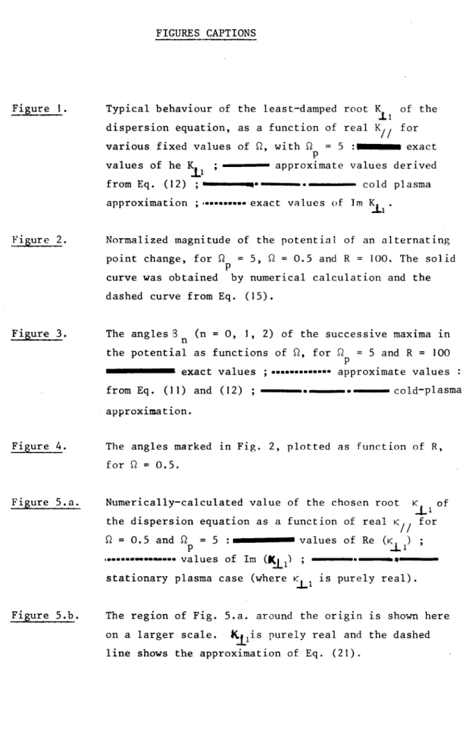
In Fig. 1 curves are plotted of the real and imaginary parts of
KL19 as functions of K,,, for fi = 5 and for various values of fi. For each of thèse values, three curves are plotted : the cold-plasma approximation given by Eq. (9), the L.T.A. approximation, and the exact curve derived numerically.
- 13 -
The L.T.A. approximation involves assuming
where a is the correction coefficient that takes account of the thermal effects25 ':
It is important to note that a vanishes for a particular value fi of fi which dépends only on � ; for � = 5, we have S2 oc 0,692. When fi � �
(e.g. � = 0.1 and � = 0.5), the coefficient a is positive and the L.T.A. curves lie below the cold-plasma straight line, which is inclined at the angle 3 to the négative Re Ki - axis. When = � , the coefficient a vanishes and there is no interférence structure : the L.T.A. approximation fails to predict any thermal effects. When fi � fi
(e.g. fi =
0.9), a is négative and the L.T.A. curve lies above the cold-plasma curve. Thus the nature of the L.T.A. approximation dépends on whether the normalized fre- quency is greater or less than � ; the physical significance of this value has not yet been identified.
The results of our numerical calculations are plotted as curves of Re
Ki and of Im K. versus K for positive real va Lues of this variable. Thus they refer to inhomogeneous waves with Im K,, = 0, rather than to the homogeneous waves (i.e. waves in which the vectors Re (K) and Im (K) are parallel to one another) that hâve been studied by some previous authors26. Our results are similar to the L.T.A. approximation for fast electrostatic waves (K rb 0) in a range of
K,,
which dépends on fi. When fi
� fi the curve of Re K is well approximated by Eq. (12), while the curve of Im
Ki is very close to the KII - axis up to a certain
value of
K, ,
which increases with increasing frequency. Above this value, the curves derived from Eq. (12) do not bend in the right direction. When
� =
fi , the exact curve of Re Ki lies below the cold-plasma straight line over a large range of
Re Ki from Eq. (12) bends in one direction only, whereas the exact curve is more complex and lies above the cold-plasma line for small
K , ,
and below it for large
KII ; thus thë discrepancies
between thèse two curves are now very significant. Moreover, the value of
K, , above which Im
Ki can no longer be ignored now decreases with increasing frequency. In short, the L.T.A. approximation does not give a good account of the behaviour of the least-damped waves when the frequency is near the gyrofrequency ; however, précise information about its range of validity can be obtained only by numerical calculation of the potential.
THE POTENTIAL CREATED BY AN ALTERNATING POINT CHARGE
The preceding three sets of curves for the least-damped root of the dispersion relation lead to very différent potential distributions near the lower oblique résonance.
Let us recall that, in the cold-plasma approximation, the potential is18
It is infinité on the résonance cône, which has a semi-apical angle 3 and it decreases smoothly with increasing 18 - 3 on both sides of this cône.
In contrast, the L.T.A. approximation for the potential is
where
F(zT) is a function defined and graphed in Réf. 10 ; its argument, which is purely real, is
- 15 -
The prédictions of the L.T.A. approximation differ from those of the cold-plasma approximation in three main respects. Firstly, the potential remains finite on the résonance cône. Secondly, this maximum of potential occurs at a slightly différent angle :
The amount of the change in the angle at résonance dépends both on the frequency and on the électron temperature(it is proportional to T
1/3), but its sign dépends on the frequency alone : the L.T.A. résonance cône lies inside the cold-plasma résonance cône if � � � , and outside it if � � � . Thirdly, there appears a quasi-periodic interférence structure, in which the minima are zéros and the maxima decrease in amplitude with increasing angular distance from the résonance cône. The angular positions of thèse secondary maxima are approximately
where n = 1, 2, 3,... Again, their angular spacing dépends on fi and is proportional to T
x/3. The entire structure occurs inside the L.T.A. résonance cône when fi � � and outside it when fi � � . In the rest of
a a
this section we shall compare thèse prédictions of the L.T.A. approximation with the results of our more précise numerical calculations, in order to establish whether or not the L.T.A. formulas are adéquate for diagnostic purposes.
When the électron température is such that R » 1, the L.T.A. approximation leads to a potential distribution in reasonably good agreement with the more précise calculations so long as the excitation frequency is not too close to the électron gyrofrequency, or more exactly, so long as fi �� fi . This fact is illustrated in Fig. 2, where the variations of \ip\ given by our computer programme (solid curve) and by Eq. (15) (dashed curve) are plotted for the case
where fi =
that the damping of the maxima at
3 and 81 is underestimated by the L.T.A. approximation ; moreover, the prédiction that the minima should be true zéros is not confirmed by the numerical calculations. We hâve verified in numerous instances that thèse slight discrepancies presist
for other values of � , of R and of � ; probably they are due to the fact that the damping of the electrostatic waves is neglected in the L.T.A. approximation.
Let us now consider how the potential distribution in the plasma changes as the normalized excitation frequency � varies from 0 to 1. In Fig. 3, we hâve plotted the angles 3 , and 3 of the successive maxima of the potential distribution as given by our programme (solid
curves) and by Eq. (17) and (18) (dashed curves) for the case where R = 100. The true résonance cône (i.e. the maximum at 30) always lies inside that given by the cold-plasma approximation, contrary to the resuit given by the approximate L.T.A. formula of Eq. (17). As regards the secondary maxima
at 3j and 32 the corresponding formula of Eq. (18) again disagrees with our more précise calculation which show that this interférence struc-
ture always lies inside the résonance cône. Moreover, as the frequency approaches the gyrofrequency, the amplitude of each of thèse secondary maxima diminishes progressively, in comparison with that of the main maximum on the résonance cône : the higher the order of the secondary
maximum, the more rapid is the decrease. In the particular case of Fig. 3, no secondary maxima are discernible when fi is greater than about 0.8. Thus exact numerical calculations of the potential show that the validity of the L.T.A. approximation dépends not only on the température but also on the frequency.
When the excitation frequency is fixed in relation to the gyro- frequency, the potential distribution due to a point charge is strongly affected by variations of the électron density or température of the plasma. For brevity, we now limit our study to the influence of the tem- pérature, and to the particular case where � = 0.5 and �
=5. Fig. 4 shows how the angles
6, 3 and 3 vary when the Larmor radius is increased from 0.001 r (R = 1 000) to 0.1 r (R = 10) ; the results of the numerical intégration for the potential hâve been plotted as the solid curves, while Eq. (17) and (18) yield the dashed curves. Thèse two sets of curves agrée
- 17 -
qualitatively. However, Eq. (17) yields too small a value for 3 , o while Eq. (18) gives too large a value for 3 especially when k is
small. Thèse two errors add constructively in the calculation of the interférence-structure spacing 3 - so when measurements of this
o 1
spacing are interpreted using the L.T.A. approximation, the estimated température is too high.
Now if the électron température is to be determined accurately, the potential measurements must be made at a distance from the source at which the interférence spacing is very sensitive to variations of this température. For instance, if Q
P
=5 and fi = 0.5 (Fig. 4) this condition is fulfilled if R � 100, in which case 3 - 3 varies rapidly as a func-
o 1
tion of R ; a measured interférence spacing of 20° would then be inter- preted as corresponding to R = 60 on the basis of our numerical results, but as R = 48 by the L.T.A. method based on Eq. (17) and (18). The latter yields a température which is about 56 % higher than the true value. This resuit is typical, and we conclude that the L.T.A. formulas are inadéquate for determining électron temperatures 26
Under most expérimental conditions, the électron density is not known in advance, but it can be deduced, together with the température, from joint measurements of the interférence spacing and of the résonance cône angle. We find that the errors in density introduced by using Eq. (17) and (18) are greatest for values of Q
near 1, where the potential
dis- tribution is strongly affected by density variations. For instance, some potential measurements in the auroral ionosphère by Gonfalone28 yield T = 655° K and n = 7.8 x 104 cm-3 (fi = 1.82) when interpreted by means of the formulas of Eq. (17) and (18), but T
= 569° K and n = 13.1 x 104 cm-3 (fi
=
2.36) when our computer programme is used. To facilitate extensive interprétation of the angular variations of
the potential we hâve drawn up a set of charts on which lines corresponding to constant values of the angles 8,3,3,... are plotted in the
0 1 2
(T , n ) plane ; pairs of values of électron température and density, together with error bars, can be read off easily from thèse charts.
IV. DRIFT EFFECTS IN A COLD MAGNETOPLASMA
In a moving magnetoplasma, the dispersion équation for electros- tatic waves is modified by the Doppler effect, so the interférence struc- ture in the potential distribution due to an alternating point charge is sensitive to the motion. To study this effect near the lower oblique résonance, we assume that the plasma is drifting in the direction of the applied static magnetic field
(V,, � 0) and we neglect the dissipative processes, namely thermal motion and collisions. The dispersion équation of the electrostatic waves is then derived from that for a stationary magnetoplasma, as given by Eq. (7), by replacing w by co - k.. V.. (i.e. n by fi - K ,-) . Thus
and the expression for the potential becomes
+00
where Ki is the root of Eq. (18) with a positive imaginary part (the choice of root when both are purely real is explained below). In this section, we first discuss how Ki varies when K the real variable of intégration, varies from -°° to +°° ; then we présent both exact numerical and approximate analytic calculations of the potential given by Eq. (19).
THE ROOT OF THE DISPERSION EQUATION
From Eq. (18), the roots of the dispersion equation29 D(fi, K) = 0 are given by
- 19 -
which shows that they vanish for �, , = 0 or fi ± 1 or fi ±
fi and go to f 00 for
k, , = fi or fi ± fi .
Thèse eight particular values - marked by dots on the vertical axis in Fig. 5. a - delimit nine branches of
the curve Ki (K//), on each of which k, has two possible values, of opposite sign, which are either purely imaginary (when Ki is négative) or purely real (when
Ki is positive).
In the first case, we take only the root with a positive imaginary part ; there are four such branches (the dotted lines in Fig. 5.a.), on ail of which the waves are strongly damped and make no appréciable contribution to the potential. In the second case, the sign of Ki is chosen by introducing an infinitésimal amount of colli- sions, and we find that it is positive when � �
Ki/ �
fi + 1 or fi-fi � k, , �fi-fi , but négative when fi+fi � K//
�
fi+fi or fi-1 � k, ,
� 0 or 0 � K,, � fi (the solid lines in Fig. 5.a.). To thèse five branches correspond five sets of undamped waves, ail of which hâve to be considered
in a quantitative analysis. However, the numerical calculation of the po- tential in the next subsection will show that the drift effect can be ana- lyzed qualitatively by considering only the two branches that start at the origin K = 0.
Thèse two, which are shown in greater détail in Fig. 5.b. (solid lines), are deformed versions of the two sole branches that exist when the plasma is stationary (broken lines). They are tangent to the latter at the origin, so they may be expected to make the principal contribution to the potential at and near the lower oblique résonance. Because the curves Ki
(K//) for a drifting plasma lie below the corresponding straight line for a stationary plasma, it follows that the résonance cône becomes narrower downstream and wider upstream when the plasma drifts. (For the relationship between the dispersion curves and the resonance-cone angle, see Réf. 26). An approximate expression for the parts of thèse curves nearest to the origin may be obtained by expanding the right-hand side of Eq. (20) as a power séries, and taking just the first two terms12 :
The corresponding curve is plotted as a dashed line in Fig. 5.b. for the case
where fi
= 5 and � = 0.5. There are discrepancies from the exact curve when
IKIII is so large that the second-order term in Eq. (21) is no longer small compared with the first-order term. Roughly speaking, the approximation is reasonable when
(y = 4.55 in the case of Fig. 5.b. so this inequality is
IK,11
« 0.37). Subject to this condition, Eq. (21) should be useful as the basis for an approximate analytic study of how the frequency variation of the potential at a fixed point is modified when the plasma drifts. But before doing this, we présent the results from a précise numerical study of the same question, in the course of which we confirm that the main résonance and other regular features of the frequency variation are indeed attributable to the two branches of the dispersion curve Ki (K that start at the origin.
NUMERICAL CALCULATION OF THE POTENTIAL
Since it has been suggested that the field-aligned drift velo- city could be deduced from the shift in frequency that occurs when the emitting and receiving électrodes are interchanged, we consider mainly the frequency variation of the potential at two fixed points, at equal distances from the source but in opposite directions. The calculation involves integrating an oscillating function, which we do numerically
by Filon's s method ** . The results are plotted as the thin curves of Fig. 6.a. and 6.b. for the case
where fi =
5 and p = 160. The curve ip_ in Fig. 6,a. shows the potential calculated for 3 = 150° while the curve i|j in Fig.6.b. is for 8 = 30° ; the subscript is the sign of the component of drift velocity along the line from the source (transmitter) to the point of observation (receiver), so in the first case the receiver is upstream from the transmitter, and in the second it is downstream. When the plasma is stationary, the curve is the same in both directions and the résonance
- 21 -
frequency
is fi = 0.493. When the plasma is in motion and the receiver is upstream, the résonance frequency fi is shifted towards the lower
-0
frequencies (fi - fi ^ 0.11), and a regular interférence structure appears at frequencies below the main résonance frequency ; hère we
call the successive secondary résonance
frequencies fi ~1 ' fi ~2
etc...
When the receiver is downstream from the transmitter, thèse results are inverted : the résonance
frequency fi + is greater
than � c
(fi+ - fi ^ 0.13) and an interférence structure, in this case with only one peak, appears above fi^ + at a frequency called fi, +i Moreover, there are irregular oscillations in the low-frequency range of the curve of
�+. Thèse results are similar to those of Storey and Pottelette but our use of the Fourier transform rather than the Laplace transform enables us to identify the branches of the dispersion curve that are responsible for the irregular oscillations of the potential downstream from the transmitter30.
The contribution made by each of the nine branches of the dispersion curve to the potential can be analyzed quantitatively by restricting of Eq. (19) to the corresponding range of the variable K To begin with, we consider the contributions from the two branches that start at the origin
k, , =
0, so we perform a partial intégration from fi-1 to 0 for �
_ and from 0 to fi for ty The thick curve in Fig. 6.a. shows the resuit of such an incomplète calculation of the potential \p_ upstream from the transmitter, obtained by considering only the contri- bution from the branch fi-1 �
k,,
� 0. Comparison with the exact curve of \\\) shows that the
frequencies fi o , fi ~i , fi ~2
of the successive maxima are only slightly modified in spite of the discrepancies in their magni- tudes. Similarly, the resuit of the partial intégration from 0 to � for the
potential ty+ downstream from the transmitter is sketched as the thick line in Fig. 6.b. Hère again, the characteristic frequencies of the main résonance and of the regular interférence structure are practically unaf- fected. Moreover the irregular oscillations are suppressed, so we conclude that they are due to undamped electrostatic waves with wave vector components
K// outside the range from 0 to fi, interfering with the waves for which the K// lie in this range. Thèse results are consistent with the notion that the waves with relatively large K only contribute to the potential downstream from the transmitter, because their group velocity vectors V are such that V . V � 0. Thus, in order to study the shift in résonance frequency and the ^s a,
interférence-structure spacing, it is sufficient to confine our attention to the branches fi-1 �
ANALYTIC APPROXIMATION FOR THE POTENTIAL
In the light of the preceding subsection, we limit the
intégration for the potential to a single branch of the curve Ki (K/ /), but some further approximations must be made before we can perforai this intégration analytically :
(i). The first approximation is to use the Eq. (21) for Ki
. Assuming that
we hâve
| p . Ki 1 »
1 at both limits of the range of K,,1
where the approximation (21) is valid ; thèse limits are defined by the inequality (23). By using the saddle-point method together with the asymptotic expan- sion of the Hankel function, we find that the corresponding frequency range of validity for Eq. (21) is
(ii). The second approximation is to extend the outer limit of intégration for the potential from fi-1 to -°° for �_, and from � to + °°
for ty This is correct if the range of «,,
where the Eq. (21) is valid is entirely included in the interval between fi-1 and fi, which implies that the frequency is such that
- 23 -
On this condition, we may neglect
K// in the non-oscillatory
term in the integrand of Eq. (19) ; the latter may then be rewritten
Using a method due to Kuehl12, we evaluate this intégral by splitting it into two parts, as follows :
where
(iii) The third approximation is to neglect the contribution of I . This final approximation is valid if
From hère on, we shall refer to thèse three assumptions collectively as the low-drift analytic (L.D.A.) approximation.
In this approximation, the potential created by an alternating point charge is
The new intégral on the right hand side dépends on]y on the parameter Sf = pi" ' Y- (P//±P|COtgB ) and can be rewritten
where$(ç ) is an intégral which may be evaluated by using a new variable of intégration t =
ipLyKil2 and by changing the upper limit of intégration from ioo to +0031 :
By developing the exponential as a power séries and using the intégral définition of the gamma function (r)32, one obtains the following séries expansion :
The asymptotic forms of Eq. (35) may be derived by the method of steepest descents ; they are
- 25 -
The procédure for evaluating is similar, except that is replaced by �_ and i is replaced by - i ; thus is the complex conjugate
of$+(Ç_). The modulus of �is graphed versus ç+ in Fig. 7. By inser- ting this function into Eq. (33), we obtain
This is the L.D.A. approximation for the potential.
Let us now use this resuit to dérive approximate formulas
for the resonance-frequency shift and the interférence -structure spacing. At a fixed angle 3, with the frequency varying, it is more convenient to use the expression
which applies when � � � . Since this approximation is linear, the shift of the résonance frequency, for a given drift velocity has the same magni- tude (but opposite sign) downstream and upstream from the transmitter. The
function
|*+(Ç+) is maximum for ç+ =
2.199, so the differential shift (i.e. the différence between the downstream and upstream résonance frequencies, which is what one would measure experimentally) is
In the limiting case where the plasma density is infinité
(fi ��°°) ,
we hâve fiT ^ fi and fi % sin 3 ;
A similar resuit has been derived previously by Pottelette33, and we hâve expressed ours in the same form ; however, he gives the numerical factor before the bracket as 2. An analytic formula also can be derived for the first frequency interférence spacing when the angle is fixed, using the fact that the first secondary maximum of |$(Ç ) |oecurs for Ç
=
5.4 ; in the limiting case where
fi -�00, we find
In the analogous formula derived by Pottelette33, the numerical factor is 1.0. Similar approximations can be derived readily for the. résonance angle shift and interférence-structure spacing at fixed frequency.
To summarize, our analysis based on the L.D.A..ippi-oximation leads to results of the same functional form as those previously published, but of slightly différent magnitude. In particular, we confira that the shift in the résonance and the interférence spacing due to the drift a long the magnetic field are proportional, in a cold magnetoplasma, to the square root of the drift velocity. It is important to reconcile :hi:: resuit with the linear proportionality discovered by Kuehl12 in che case of warm drifting magnetoplasma.
- 27 -
V. COMBINED EFFECTS OF THERMAL AND DRIFT MOTIONS
In this section, we consider how the potential distribution created in a warm magnetoplasma is modified by the joint action of the thermal and drift motions, which hâve been treated separately in the two preceding sections. Downstream from the transmitter, the effects of both thèse motions are to close up the résonance cône and to create a regular interférence structure within it. Upstream from the transmitter, the thermal motion has the same effect, but the drift motion opens up the résonance cône and gives rise to a regular interférence structure outside it. In studying the résultant potential distribution, both analytically and numerically, we again neglect ions and collisions and adopt the least- damped-root approximation. Analytically, Kuehl12 has already derived some approximate formulas on the further asumption that
ri « a2 r Vy3 z3 we find that his method of calculation is also applicable to the case where
ri » a2 r ,Vy3 �3 Numerically, of course, it is possible to calculate the potential distribution for arbitrary values of the thermal and drift velocities . In this section, we first analyze the behaviour of the least-damped root of the dispersion équation for electrostatic
waves in a drifting Maxwellian magnetoplasma, then we complète the analytic calculations of Kuehl for the case where
ri » a2 r Vy3 9.3, and finally we présent the results of some numerical calculations of the potential.
THE LEAST-DAMPED ROOT OF THE DISPERSION EQUATION
In Fig. 8, the exact values of Re K,
(thick solid line) and of Im
K. (thick dashed line) are plotted as functions of K//, for fi =5., fi = 0.5 and
£ /r = 0.25. The corresponding purely real values of Ki for a stationary cold plasma are also graphed, as the thin broken line, while the thin solid line represents a purely real approximation to K( , inclu- ding thermal and drift effects, which we shall use in our analytic calcu- lation of the potential.
This approximation for Ki
is obtained by expanding the complète dispersion équation - Eq. (2) - as a power séries in terms of the variables K. and K,,. Near the origin K ^ 0, it is sufficient to retain only the three leading termes, so
where a and y are defined by Eq. (13) and (22) respectively. In this approximation, the thermal and drift effects are not coupled, inasmuch as the expression for K. is the sum of the thermal correction term from Eq. (12) - illustrated in Fig. 1 - and the drift correction term from Eq. (21) - illustrated in Fig. 5.b. - added to the expression of Eq. (8) for the case of a cold stationary plasma. For positive values of
K,,,
the curve representing this approximation to the least- damped root always lies below the cold-plasma straight line (as in Fig. 8)
if a � 0, i.e. if � � fi . When � � �� 1, this curve lies below the straight line if
K,,
�
yr./a and aboue it if K,,
� yr /al. For négative
values of
K, ,, the situation
is as follows : when fi
� fi , the approximate curve leaves the origin below the cold-plasma straight line, then
crosses this line at the point where
K,, = - YrT /al and thereafter lies above it ; when fi
� fi � 1, the curve always lies below the line. Thus the behaviour of the least-damped root, as given by this low température and drift (L.T.D.) approximation, dépends not only on the relative values of the thermal and drift velocities but also on the frequency.
The exact values of Ki , calculated by using the itérative complex-root-finding method described at the end of section II, are similar to the preceding approximate values only for fast electrostatic waves with K � 0. For large values of |K,,|, the discrepancics that hâve been described separately in sections III and IV now occur jointly. Uepending on the frequency fi and on the sign of
K.//» the disagreements
due to the thermal and drift effects either add to or substract from one another, and so reduce or enlarge the range of
K,,,
around the origin, within which Eq. (43) is valid. The imaginary part of Ki can be ignored inside this range35, but not outside it. Just as for the L.T.A. and L.D.A. approximations developed previously, no general expression can be given to specify the range of validity of the L.T.D. approximation.
In the particular case illustrated by Fig. 8, it appears that Eq. (43) is a good approximation when
Ik.,1 � 0.1. The range of validity is somewhat larger for négative values of
K,, than for positive
values. Hence an approximate analytic calculation of the potential., based on Eq. (43), should give better results upstream than downstream.
- 29 -
Because our itérative method for finding complex roots starts from the origin K = 0, we must assume that the electrostatic waves what were responsible for the irregular oscillations of the potential in the case of a cold drifting magnetoplasma are damped by thermal processes. In other words, the imaginary part of Ki is assumed to be much greater than its real part along the corresponding branches of the dispersion curve. Thèse branches occur outside the range (fi-1) �
K,,
��, which contains the least-damped ones (Fig. 5.a.). The définitions adopted
in section II for the normalized wavenumbers involve K,,
=
(rL 19,) K,/, so thèse branches occur for négative
K..
� (fi-1)
r /l and for positive K,, �
fi
r / £ . Since the limits of thèse ranges dépend both on the nor- malized frequency fi and on the ratio
r / £ , the same must be true of the range of validity of the above assumtion. Again, it seenis impossible to give a general expression to specify this range.
ANALYTIC CALCULATION OF THE POTENTIAL
The angular shift of the résonance cône due to field-aligned drift in a Maxwellian magnetoplasma has been calculated analytically by Kuehl. He did this by expressing the potential created by an alter- nating point charge as a power séries in the variable
e =
R i * ' 3 |a| _2/3y £ /rT , and by assuming only the first-order terms, on the assumption that E
v « i.e. that
ri- « a2 r Vy3 l3 . Then he calculated approximately the new value of the variable
z for which the magnitude of the potential is ma- ximum, namely zT = 1.800 + 0.906
e ; remember, from its définition by Eq. (16), that
z is proportional to the angular drift of the résonance at fixed frequency.
In the case where the angle is kept fixed and we sweep the frequecy, it is more convenient to use the following expression for
z near the résonance frequency :
Hence, the résonance frequency in a stationary Maxwellian plasma is
Like the angular shift at fixed frequency, the résonance frequency shift
fi o - fi c is proportional to
r2'3, L and so to T e 1/3.
In the présence of field-aligned drift, there is an additional shift which changes its sign when the emitting and receiving électrodes are interchanged. As in section IV, the résonance frequency will be called
fi + when
the receiver is upstream,
and H "o
when it is downstream from the transmitter. The average of thèse two frequencies is still fi .
o Experimentally, one measures their différence
where a and y are calculated at the frequency � = � . This differential shift is proportional to
i/r. 2'3ri 1 /3 , and so to the ratio Vr // /v th 2/3 (rUb) 1/3
By following Kuehl's method, it is easy to calculate the same parameters
fi and
Afi in the other limit where
ri �� a2 r.Vy3 ^3 Downstream from the transmitter, the use of Eq. (43) for
k,
= 1 l/r, leads to a new intégral for the potential :
By séries expanding the exponential containing the thermal correction term -
- 31 -
�is the function defined in section IV and Er =
Pl 1/2 y- 3/2 (xrL/9, 2 2 Assuming ET « 1., i.e.
r. »
ot 2 rL 1/yly3@ we may retain only the first two terms of the séries. From numerical calculations
of$and of its derivatives, together with a séries expansion about the value Ç = 2.199 for
which |$| is maximum, we find that the maximum magnitude of the potential occurs when Ç = 2.199 + 0.128 e . The analytic calculation of the potential ip_ upstream from the transmitter is similar ; its magni-
tude is maximum for ç- = 2.199 - 0.128
eT. In each of thèse two formulas, the constant term, which has been derived already in section IV, represents the main effect of the drift motion : the second term represents the smaller additional effect of the thermal motion. Together, thèse formulas show that the differential shift in résonance frequency due to the drift motion,
Afi = 2+0 -
is not affected by thermal motion while the average reso- nance frequency
(fi^ + o + fi ~o )/2 which
we shall now
call � , a is
Thus the average résonance frequency is shifted proportionally to the ratio rT 2 /l - and so to T - due to the thermal motion ; while the differential shift in résonance frequency due to the drift is proportional to V,, ' , like in the cold-plasma case.
Before confronting thèse approximate results with the numerical results from our computer programme, we should point out some peculiarities of this analytic approach devised by Kuehl. His first step is to approximate the least-damped root of the dispersion équation. The errors that this involves hâve been discussed in the preceding subsection. The second step is to introduce a référence function by taking into account only one major effect, either that of the thermal motion or that of the drift motion. In so doing, the asymptotic expansion of the Hankel function is used in such a way that, when one calculâtes the potential, one cannot recover the case of the cold stationary magnetoplasma : note
that when R - - (corresponding to T - 0) in Eq. (15), or when p -+ °° (corresponding to V,, 0) in Eq. (38), senseless results are obtained.
Moreover, the argument of this référence function is approximated near the résonance angle or frequency, and more errors are introduced thereby. The third step consists of expressing tlie potential as a power séries in a parameter that takes account of the minor effect. The two infinité séries obtained by starting from the one or the other référence function are strictly équivalent and include a coupling between the thermal and drift effects. Then, in a final set of approximations, the treatment of this coupling is simplified by truncating the séries which amounts
to ignoring the influence of the minor on the major effect, but not the converse. The errors committed at thèse successive steps of the analytic calculations can either reinforce or cancel one another, so it would be difficult to obtain any simple and global criterion of validity of ail the approximations by comparison between the final approximate results and the exact numerical results.
NUMERICAL CALCULATION OF THE POTENTIAL
It is easy to modify our computer programme for calculating the potential created by an alternating point charge in a Maxwellian magnetoplasma, so as to introduce a field-aligned drift. In Eq. (4) for
a , the term involving the ratio l/r is now non-zero, and the numerical intégration of Eq. (5) must now be performed from - - to + °°
since Ki (K, ,) ^ Ki (- K,,). Limiting ourselves to the case where only the excitation frequency is varied, we shall présent one example of a numerical calculation of the potential with fi varying from 0 to I., before focussing our attention on the resonance-frequency shift due to the plasma drift.
Fig. 9 shows the numerically-calculated frequency variations of the magnitude and phase of the potential at each of two fixed points, at equal distances from the source but in opposite directions. The parameter values are as given in the figure caption. At frequencies greater than the
résonance frequency, ail the curves shows an interférence structure which is a thermal effect. In the amplitude curves, this structure is not suffi- ciently pronounced to produce actual maxima and minima, but such extrema appear distincly in the phase curves. The relative smoothness of the curves for �_ leads us to think that the interférence structure due to the drift is damped by the thermal motion. The remaining - and most important -
- 33 -
effect of the drift is to shift the résonance frequency : in Fig. 9, the differential shift Afi is 0.522 while the approximate formulas (40) and (46) give 0.1185 and 0.0303 respectively. Since r-L = 1.2 m and
a r /y £ = 1.17 m, we are roughly in the intermediate range where neither of the approximate formulas is valid. Thus we hâve hère a case where the exact differential shift due to the drift lies between the asymptotic values given by the two analytic calculations, though this is no true in every case.
In fact, the drift effect is systematically underestimated by using the L.T.D. approximation for the least-damped root of the dispersion équation, but this basic inadequacy is subsequently attenuated by the further approximations made in the analytic calculation of the résonance frequency shift. In Fig. 10, the variations of the differential frequency shift Afi are graphed versus in the case
where fi P
= 5., r = . 8 m and 8 = 30° or 150°, for R = 30, 50 and 100, and also for R - °° which is the cold-plasma case. The solid curves show the variations calculated numeri- cally with our complète computer programme, in which the least-damped root Ki of Eq. (2) is determined by the itérative complex-root-finding method ; the dashed curves are the approximations, obtained from Eq. (46) when R is finite and from Eq. (40) when R is infinité. In this example, Eq. (46) gives a differential frequency shift Afi less than the exact value when R is large and greater than the exact value when R is small. We note that this resuit is consistent with the L.T.D. approximation which is valid when the distance is both large enough to justify the use of the
low-temperature approximation and small enough to satisfy the condition ri « a r 1*/y3 £ 3. On the other hand, the exact values of Afi vary more or less linearly with £ , even for large values of R ; this resuit disagrees with the prédiction of Eq. (40), which is plotted as the dashed curve
labelled R = °°, according to which Afi should be proportional to tl/2. Generally speaking, Eq. (40) seems to be more of theoretical than of practical interest since the conditions for it to be applicable do not occur in the expérimental situations that we envisage. In this example, where � = 30° (or 1500), Kuehl's formula for Afi would be useful for data analysis, but we use of the numerical values for Afi would improve the accuracy.