HAL Id: hal-01878765
https://hal.archives-ouvertes.fr/hal-01878765
Preprint submitted on 21 Sep 2018
HAL is a multi-disciplinary open access
archive for the deposit and dissemination of
sci-entific research documents, whether they are
pub-lished or not. The documents may come from
L’archive ouverte pluridisciplinaire HAL, est
destinée au dépôt et à la diffusion de documents
scientifiques de niveau recherche, publiés ou non,
émanant des établissements d’enseignement et de
Fractional decomposition of matrices and parallel
computing
Frédéric Hecht, Sidi-Mahmoud Kaber
To cite this version:
Frédéric Hecht, Sidi-Mahmoud Kaber. Fractional decomposition of matrices and parallel computing.
2018. �hal-01878765�
Fractional decomposition of matrices
and parallel computing
Fr´ed´eric Hecht, Sidi-Mahmoud Kaber
Sorbonne Universit´e,
Universit´e Paris-Diderot, CNRS,
Laboratoire Jacques-Louis Lions,
LJLL, F-75005 Paris, France
September 21, 2018
Abstract
We are interested in the design of parallel numerical schemes for linear systems. We give an effec-tive solution to this problem in the following case: the matrix A of the linear system is the product of p nonsingular matrices Am
i with specific shape: Ai= I − hiX for a fixed matrix X and real numbers hi. Although having the special form, these matrices Aiarise frequently in the discretization of evolution-ary Partial Differential Equations. The idea is to express A−1as a linear combination of elementary matrices A−ki . Hence the solution of the linear system with matrix A is a linear combination of the solutions of linear systems with matrices Aki. These systems are solved simultaneously on different processors.
1
Introduction
Let X be a real n × n square real (or complex) matrix and (hi)pi=1a collection of pairwise distinct real
numbers. Matrices of the shape
Ai= I − hiX (1)
with I the n × n identity matrix, appear in many numerical schemes for differential equations. For small hi(discretization parameters), such matrices are nonsingular. So is matrix
A =
p
Y
i=1
Ami (2)
for any m ∈ N. Note that matrices Aicommute and A is a polynomial of the single variable X. The
problem of interest here is the following: given y ∈ Rn, compute the unique solution x ∈ Rn of the linear system
Ax = b (3)
using several processors at our disposal. The aim is to use parallel computing to save computational time. The key idea consists in expressing matrix A−1 as a linear combination of matrices ((A−ki )pi=1)m
k=1.
Since matrices Ai we consider come from the discretization of differential equations by time implicit
scheme, our method falls into the family of “parallelization in time” algorithms. We refrer to [3] for a comprehensive overview of parallel time integration methods.
• In section 2, we present the algebraic problem to be solved.
• In section 3, we explain how the method can be used to solve homgeneous evolution equations ut= Lu.
• In section 4, we consider nonhomgeneous evolution equations ut = Lu + f and derive a new
parallel algorithm to solve such problems.
• The last section contains remarks on the reliability of the method and its limitations.
All computations have been done using FreeFem++, a Finite Elements software for the discretization of Partial Differential Equations [1].
2
The algebraic problem
We consider in this section the homogeneous linear time-evolution problem
ut= Lu. (4)
Section 4 is devoted the nonhomogenoeus case which requiers a different numerical treatment. Starting from an initial data u0, the time discretization of this equation by implicit Euler scheme with time step
h1reads
u1− u0
h1
= Lu1. (5)
Solving (5) with a Finite Difference scheme gives
(I − h1X)u1= u0. (6)
with X a Finite Difference approximation of the spatial operator L. Iterating p steps of the implicit scheme, we obtain an equation for up
(I − hpX) · · · (I − h2X)(I − h1X)up= u0.
We will always assume the time steps hismall enough insuring that all matrices Aiand A
A =
p
Y
i=1
Ai (7)
are nonsingular. Hence upis given by
up= A−1u0.
Here comes into play the fractional decompositions of matrices. Indeed, if the hi are piecwise distinct,
there exist p real numbers (αi) p
i=1such that
A−1=
p
X
k=1
αiA−1i . (8)
Consequently, the vector upcould be split into
up=
p
X
i=1
each xibeing the unique solution of the system
Aixi= u0. (9)
These p linear systems are independent each other allowing the computation of up by using p proces-sors to compute simultaneously the xi. This idea has been applied in [2] to solve the two-dimensional
heat equation discretized by a Finite Difference scheme. Note that the αi involved in (8) have a simple
expression
αi=
Y
k6=i
(1 − hk/hi)−1. (10)
We introduce now the general case where the matrix A to be inverted is definied by (2) with Aidefined
again as in (1). We will always assume that the hiare piecewise distinct.
Proposition 1 There exist mp real numbers αi,ksuch that the inverse ofA defined in (2) is
A−1= p X i=1 m X k=1 αi,kA−ki . (11)
This is just the partial fraction decomposition of rational functions written for polynomials of matrices. According to (11), the unique solution x of the linear system (3), with A defined in (2), is decomposed as
x = p X i=1 xi. (12) with xi= m X k=1 αi,kxi,k. (13)
and xi,kbeing the unique solution of the linear system
Akixi,k= b.
The computation of each xiis done on one processor allowing the parallelization of the algorithm. Here
is an efficient way to do so: On processor number i,
? compute xi,1solution of Aixi,1= b,
? compute xi,2solution of Aixi,2= xi,1,
.. .
? compute xi,msolution of Aixi,m= xi,m−1,
? lastly, compute xiby (13).
(14)
Computation of the solution x by (12) requiers communications between processors. This step maybe very time consuming, especially if the amount of data to transfer is large.
We end this section with numerical issues. The coefficients αi,kin (11) are given by
αi,j= 1 (m − j)! t→1/hlimi [(t − hit) m ϕ(t) ] (m−j). (15) with ϕ(t) = p Y i=1 (1 − hit)m.
For m = 1, formulas (15) reduces to (10). For m = 2, there exist also simple explicit formulas : A−1= p X i=1 αi,1A−1i + αi,2A−2i (16) with αi,2= Y j6=i 1 (1 −hj hi) 2, αi,1= −2αi,2 X j6=i hj hi− hj . (17)
For m > 2 there is an alternate method to the computation of the mp coefficents αi,kby (15): solve the
following linear system for well choosen mp real numbers t` p X i=1 m X k=1 1 (1 − hit`)k αi,k= 1 ϕ(t`) , 1 ≤ ` ≤ mp. (18)
In other words, compute the coefficients αi,kby interpolation of the function 1/ϕ at the distincts nodes
t`(to be well choosen). With αi∈ Rmand α ∈ Rmpdefined by
αi= αi,1 .. . αi,m , α = α1 .. . αp ,
the linear system to solve is ψ1(t 1) · · · ψp(t1) .. . ... ψ1(t mp) · · · ψp(tmp) α = 1/ϕ(t1) .. . 1/ϕ(tmp) (19) with ψi(t`) = ( 1 1 − hit` , · · · , 1 (1 − hit`)m )
This system, a Vandermonde-like one, is ill-conditionned. Since only the case m = 1 was used in our numerical tests, we do not discus further the linear system (19). Of course, preconditionning of the system is necessary for larger values of m.
The main drawback of the method is that the coefficients do not have a constant sign and, in addition, may be very large, consult [2]. This affects the accuracy. Typically, only an approximation ˜xi of xi is
available: k˜xi− xik ≤ ε, from which we deduce the following estimate of the error on the solution x:
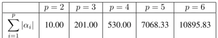
k˜x − xk ≤ " p X i=1 |αi| # ε. (20)
Since the first term, that amplifies the error, may highly increases with the parameter p, it is crucial to limit our investigation for small values of this parameter, see [2]. As an illustration, Table 1 displays the evolution of the amplification term as a function of p.
3
The homogeneous case
As was stated earlier, Proposition 1 was used in [2] (in the case m = 1) to solve homogeneous linear time-evolution equation (4) discretized by a Finite Difference method. In this section, we reproduce the
p = 2 p = 3 p = 4 p = 5 p = 6
p
X
i=1
|αi| 10.00 201.00 530.00 7068.33 10895.83
Table 1: Evolution of the amplification term in (20) as a function of the number of processors p. The hi are choosen symmetrically : c = 1/10 and in the case p = 2, hi = (1 ± c)h, in the case p = 3,
hi∈ {h, (1 ± c)h}, in the case p = 4, hi∈ {(1 ± c)h, (1 ± 2c)h}, . . .
tests in [2] using a Finite Element scheme. One iteration of a Finite Elelement Method to solve the same problem reads
Mu
1− u0
h1
= Bu1
with M the mass matrix and B the stiffness one. We obtain the same discrete evolution equation as in the Finite Difference case (6) with
X = M−1B.
As we will see in next section this is not the always the case for nonhomogeneous equations. Consider firstly the case m = 1 that will be mostly used in practice (i.e. A is defined by (7). Let T0, Tf be the
initial and final times. We define p time steps h1, h1, · · · , hpet intermediate times tn= T0+ n× (time
steps) used in a cyclical order: firstly h1, then h2, · · · , hp, · · ·
tn= T0+ h1+ h2+ · · · + hp+ h1+ h2+ · · ·
| {z }
n terms
It is important to precise that our algorithm computes the solution only at times tkp, k = 1, · · · , K by
going directly from approximation at time tkp to approximation at time t(k+1)p. Indeed, suppose ukp
known. Instead of computing sequentially
? ukp+1solution of A1ukp+1= ukp, ? ukp+2solution of A2ukp+2= ukp+1, .. . ? ukp+psolution of Apukp+p= ukp+p−1, (21)
we write u(k+1)pas the solution of the linear system
Au(k+1)p= ukp (22)
with A =Qp
i=1Aiand solve this system using the decomposition (8)-(10).
Let us compare sequential versus parallel computations.
1. Sequential solution. The cost of the sequential solution obtained by procedure (21) is the cost of solving p linear sytems
2. Parallel solution. The cost of the parallel procedure (8)-(10) is that of one linear system sinch each xiis computed in full parallel. However, we have to take into account the cost of summing up the
xito get the solution by (12). This imposes a global communication requirement between all of
the processors in order to compute and share the updated solutions. This harms the efficiency of the method.
1. Sequential solution. Solve mp linear sytems to compute x the solution of (21) with Aireplaced by
Am
i . The cost is that of solving mp linear sytems.
2. Parallel solution. On each of the p processors, compute in full parallel one xithis way:
(a) compute the xi,kiteratively:
Aixi,1= b, Aixi,2= xi,1, . . . Aixi,m= xi,m−1
by solving m linear systems, (b) add the xi,kup to get xiusing (13).
The cost is that of solving m linear sytems. Of course, there is an additional cost to take into account: the summing up the xito get x by (12).
We use a P1-Finite Element method for discretization in space and implicit Euler scheme for time discretization to solve the 2D homogeneous heat equation on a domain Ω ⊂ R2 with homogeneous
Neumann boundary conditions. The domain Ω is the unit square, the initial condition is is u0(x, y) =
cos(nπx) cos(mπy) so that the exact solution is known. The final time of all numerical experiments presented is T = 1. The computations were done on supercomputer SGI-UV2000 with 32 CPUs (Intel Xeon 64 bits EvyBridge E4650 with 10 core) using MPI parallel implementation in Freefem.
There are p processors at our disposal and we use each of them to advance in time (only once) with a time-step hi(1 ≤ i ≤ p). The linear system to solve is (2) with m = 1.
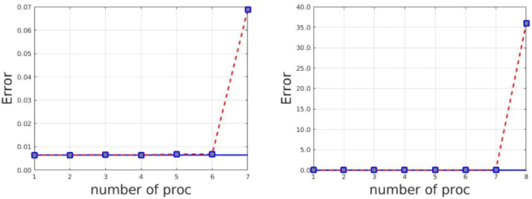
Figure 1 represents the error. The error increases with p the number of processors. Up to 7 processors, the error is constant, almost equal the error made by using one processor. Starting from p = 8, the error increases. The growth of the error is due to bad behaviour of the coefficents αi, see Table 1. As already
mentioned, we limit the use of the methos to moderate values of p. The method is therefore far from massively parallel computing!
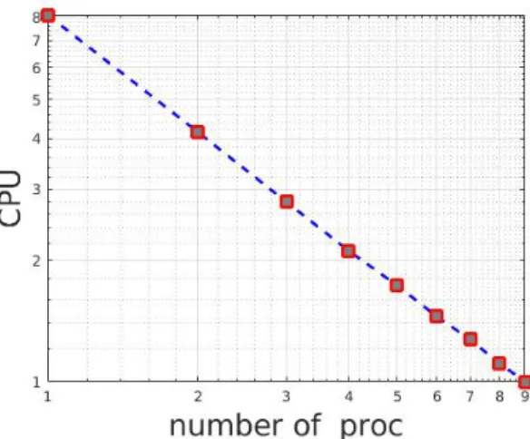
Figure 2 represents the computational time as a function of p. We observe a decreasing of computa-tional time as the number of processors increases. For example, using 6 processors instead of one, divide the computational time by a factor 5.8.
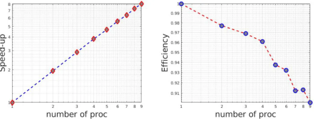
Two quantities are important in parallel computing: the Speedup defined as the ratio of sequential time over parallel time and the parallel Efficiency defined as1p×Speedup.
Both are displayed on figure 3. Ideally, the speedup should be equal to p if the communications between processors have no cost. But this is, of course, never the case. We obtain the following speedups: with 2 processors, we have a speedup of 1.95, a speedup of 3.8 using 4 processors, and a speedup of 8.2 with 9 processors. Idealy, the parallel efficiency should be equal to 1. We obtain the following results: with 2 processors, we have an efficiency of 0.98, an efficiency of 0.96 using 4 processors, and an efficiency of 0.9 with 9 processors.
The algorithm gives good results for the values of p we tested. We emphasize again that we do not plan to use our method for large values of p since the amplification term in (20) growth rapidly with p as shown in Table 1. We return to this issue in the next section.
Figure 1: The 2D homogeneous heat equation. L2 error (numerical solution versus exact solution).
Numerical parallel solution as a function of p that is also the number of processors. Solid line represents the error of the sequential solution.
Figure 2: The 2D homogeneous heat equation. CPU time (log scale) as a function of the number of processors.
Figure 3: The 2D homogeneous heat equation. Speedup (left) and Efficiency (right) as a function of the number of processors.
4
The nonhomogeneous case
Consider the nonhomogeneous Differential Equationut= Lu + f . (23)
One step in the Finite Element Method to solve (23) reads Mu
n+1− un
hi
= Bun+1+ fn+1 with M the mass matrix, B the stiffness one, and
fn+1= (hf (. , tn+1), ϕii)i,
with (ϕi)ithe Finite Element Basis. If f belongs to V, the Finite Element space, we have
fn+1= M Fn+1, Fn+1= (f (Si, tn+1))i,
with Sithe nodes of the Finite Element triangulation. In that case, we obtain the same expression as in
the Finite Difference setting with
Ai= I − hiX, X = M−1B.
We introduce now some notations to simplify the presentation: ? ∆T = mPp
k=1hk,
? Tn= T0+ n∆T and unthe approximation of u(Tn),
? Tn,j= Tn+ mP j
k=1hkand un,jthe approximation of u(Tn,j).
Note that Tn,0= Tnand Tn,p= Tn+1.
Suppose unknown, using m times the time-step h1, we get un,1solution of
Am1 un,1= un+ h1 m
X
j=1
Aj−11 f (Tn+ jh1).
Using then m times the time-step h2, we get un,2solution of
Am2un,2= un,1+ h2 m X j=1 Aj−12 f (Tn,1+ jh2). Finally Ampun,p= un,p−1+ hp m X j=1 Aj−1p f (Tn,p−1+ jhp).
So that, un+1= un,p−1is the solution of the linear system
Aun+1= un+ gn, (24) with gn= p X k=1 hkBk m X j=1 Aj−1k f (Tn,k−1+ jhk) (25) and Bk= k−1 Y `=1 Am` . The idea is to compute un+1using Proposition 1 to solve (24).
4.1
The algorithm
First version
1. For k = 0, · · · , K1− 1 (K1∆T = Tf inal)
(a) ukis known (it is an approximation of u at time Tk)
(b) Compute gkdefined in (25)
(c) Compute uk+1solution of (24) To do so
i. compute in parallel xiby (13) and (14) with b = uk+ gk,
ii. make a “reduce” step to compute uk+1by (12):
uk+1= p
X
i=1
xi.
(d) uk+1is computed (it is an approximation of u at time Tk+1= Tn+ ∆T )
It is important to point out that the algorithm computes the solution only at times Tk, k = 1, · · · , K1
by going directly from approximation at time Tkto approximation at time Tk+1. In one step, the advance
in time is equal to ∆T . Communications between the processors is done K1times (during the sommation
process).
Remarque 1 Step 1b of the algorithm may be improved. Instead of computing gkby one processor while
the others sleep, we use all processors to compute in parallel thep next right-hand sides gk0.
This leads to the following algorithm that we used in the computations. Note that, now, the outer loop is performed K2= K1/p times.
Second version
1. For k = 0, · · · , K2− 1 (K2p∆T = Tf inal)
(a) ukpis known (it is an approximation of u at time Tkp)
(b) Compute in parallel the p right-hand sides gkp+(i−1)pmfor i = 1, · · · , p.
(c) Compute sequentially ukp+ipmfor i = 1, · · · , p solution of
Aukp+ipm= ukp+(i−1)pm+ gkp+(i−1)pm
To do so
i. compute in parallel xiby (13) and (14) with b = ukp+(i−1)pm+ gkp+(i−1)pm,
ii. make a “reduce” step to compute ukp+ipmby (12):
ukp+ipm= p
X
i=1
xi.
(d) u(k+1)pis computed (it is an approximation of u at time T(k+1)p= Tkp+ p∆T )
The algorithm computes the solution only at times Tkp, by going directly from approximation at time Tkp
to approximation at time T(k+1)p. In one step, the advance in time is equal to p∆T . Communications
between all of the processors is done K2times. Thus, we have p times less parallel overhead. That is
4.2
Numerical experiments
We use a P1-Finite Element method for discretization in space and implicit Euler scheme for time dis-cretization to solve the the 2D nonhomogeneous heat equation
∂tu − ∆u = f
on a domain Ω ⊂ R2with Dirichlet boundary conditions. The domain Ω is the unit square. The source
term f is choosen so that the exact solution is u(x, y, t) = sin(nπx) sin(mπy) cos(mt). The final time of all numerical experiments presented is T = 1.
We fix m = 1 and vary p, the number of processors. Figure 4 represents the error. As already men-tioned, the error increases with p the number of processors. For p = 8 the error becomes unacceptable. Afterward, we will consider at most p = 7 processors.
Figure 5 represents the computational time as a function. We observe a decreasing of computational time as the number of processors increases. For example, using 6 processors instead of one, divide the computational time a factor 4.9.
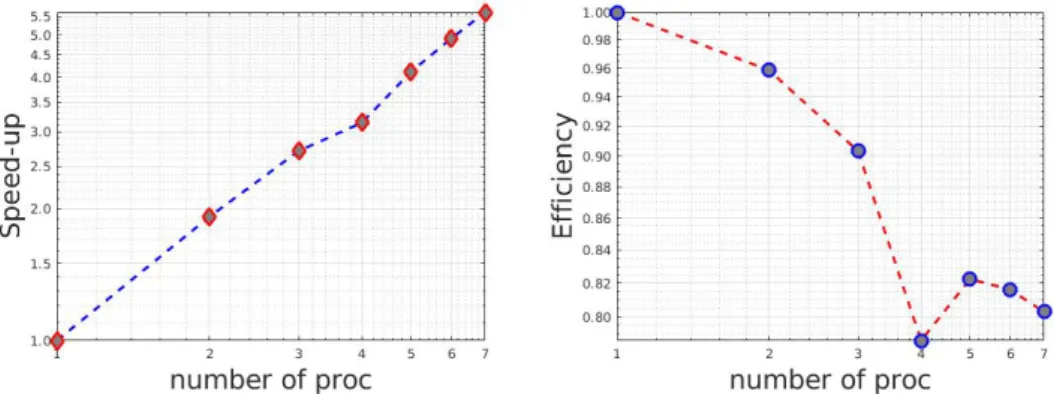
Speedup and parallel Efficiency are displayed on figure 6. We obtain the following speedups: with 2 processors, we have a speedup of nearly 1.9, a speedup of 3.14 using 4 processors and a speedup of 4.89 with 6 processors. We obtain the following results for efficiency: with 2 processors, we have an efficiency of 0.96, an efficiency of 0.79 using 4 processors and an efficiency of 0.816 with 6 processors.
Although they are less impressive than in thehomogeneous case, both Speedup and Parallel are very good. We mention again that we plan to use our method only for moderate values of p.
Figure 4: The 2D nonhomogeneous heat equation. L2error (numerical solution versus exact solution). Numerical parallel solution as a function of p that is also the number of processors. Solid line represents the error of the sequential solution.
5
Conclusion
We have extended the work initiated in [2] on the fractional decomposition of the inverse of some specific matrices resulting from the discretization of evolutionary differential equations. We apply this decompo-sition to solve nonhomgeneous Partial Differential Equations using parallel computing. Although, both speedup and parallel efficiency are good, the method is effective, for accuracy purposes, only for use on a moderate number of processors. Several developments of the method are currently investigated: analyse of the case m ≥ 2 (see discussion in Section 2), combine first order methods computed in par-allel to get a high order method, and eventually combine the method with space-parpar-allelization (domain decomposition methods).
Figure 5: The 2D nonhomogeneous heat equation. CPU time (log scale) as a function of the number of processors.
Figure 6: The 2D nonhomogeneous heat equation. Speedup (left) and Efficiency (right) as a function of the number of processors.
References
[1] F. Hecht, New development in FreeFem++. J. Numer. Math. 20, no. 3-4, 2012.
[2] S.-M. Kaber, A. Loumi and P. Parnaudeau, Parallel Solution of Linear Systems. East Asian Journal on Applied Mathematics, Vol. 6, No. 3, 2016.
[3] M.J. Gander, 50 Years of Time Parallel Time Integration, to appear in ’Multiple Shooting and Time Domain Decomposition’, T. Carraro, M. Geiger, S. K¨orkel, R. Rannacher, editors, Springer Verlag, 2015.