Self-Adapting Point Location

HAL Id: inria-00438486

https://hal.inria.fr/inria-00438486v3

Submitted on 12 Jul 2010

HAL is a multi-disciplinary open access

archive for the deposit and dissemination of

sci-entific research documents, whether they are

pub-lished or not. The documents may come from

teaching and research institutions in France or

L’archive ouverte pluridisciplinaire HAL, est

destinée au dépôt et à la diffusion de documents

scientifiques de niveau recherche, publiés ou non,

émanant des établissements d’enseignement et de

recherche français ou étrangers, des laboratoires

Pedro de Castro, Olivier Devillers

To cite this version:

Pedro de Castro, Olivier Devillers. Self-Adapting Point Location. [Research Report] RR-7132, INRIA.

2009, pp.24. �inria-00438486v3�

a p p o r t

d e r e c h e r c h e

0249-6399

ISRN

INRIA/RR--7132--FR+ENG

Self-Adapting Point Location

Pedro Machado Manhães de Castro — Olivier Devillers

N° 7132 — version 3

Centre de recherche INRIA Sophia Antipolis – Méditerranée 2004, route des Lucioles, BP 93, 06902 Sophia Antipolis Cedex

Pedro Machado Manhães de Castro , Olivier Devillers

Thème : Algorithmique, calcul certifié et cryptographie Équipe-Projet Geometrica

Rapport de recherche n° 7132 — version 3 — initial version December 2009 — revised version July 2010 — 27 pages

Abstract: Point location in spatial subdivision is one of the most studied problems in computational geometry. In the case of triangulations of Rd_{, we}

revisit the problem to exploit a possible coherence between the query-points. For a single query, walking in the triangulation is a classical strategy with good practical behavior and expected complexity O(n1/d_{) if the points are}

evenly distributed. Based upon this strategy, we analyze, implement, and evaluate a distribution-sensitive point location algorithm based on the classi-cal Jump & Walk, classi-called Keep, Jump, & Walk. For a batch of query-points, the main idea is to use previous queries to improve the current one. In practice, Keep, Jump, & Walk is actually a very competitive method to locate points in a triangulation.

Regarding point location in a Delaunay triangulation, we show how the Delaunay hierarchy can be used to answer, under some hypotheses, a query q with a O(log #(pq)) randomized expected complexity, where p is a previously located query and #(s) indicates the number of simplices crossed by the line segment s.

The Delaunay hierarchy has O(n log n) time complexity and O(n) memory complexity in the plane, and under certain realistic hypotheses these complexi-ties generalize to any finite dimension.

Finally, we combine the good distribution-sensitive behavior of Keep, Jump, & Walk, and the good complexity of the Delaunay hierarchy, into a novel point location algorithm called Keep, Jump, & Climb. To the best of our knowledge, Keep, Jump, & Climb is the first practical distribution-sensitive algorithm that works both in theory and in practice for Delaunay triangulation—in our ex-periments, it is faster than the Delaunay hierarchy regardless of the spatial coherence of queries, and significantly faster when queries have strong spatial coherence.

Key-words: Point location, Delaunay triangulation

Résumé : La localisation de points dans une subdivision de l’espace est un classique de la géométrie algorithmique, nous réexaminons ce problème dans le cas des triangulations de Rd _{pour exploiter une éventuelle cohérence entre les}

requêtes.

Pour une requête, marcher dans la triangulation est une stratégie classique de localisation qui donne de bons résultats pratique et a une complexité moyenne O(n1/d_{) si les points sont uniformément distribués.}

Basée súr telle strategie, nous alysons, implementons, et évaluons une strate-gie de localization de point adaptable aux distributions des requêtes, basée sûr Jump & Walk, appellée Keep, Jump, & Walk. Pour des paquets de requêtes, l’idée principale est d’utiliser les requêtes précédentes pour améliorer la requête courante; nous comparons différente stratégies qui ont une influence sur les con-stantes cachées dans les grands O.

Toujours à propos de la complexité d’une requête, nous montrons que la hiérarchie de Delaunay peut être utilisée pour localiser un point q à partir d’une requête précédente q avec une complexité randomisée O(log #(pq)) pourvu que la triangulation vérifie certaines hypothèses (#(s) désigne le nombre de simplex traversés par le segment s). La structure de donnée a une taille O(n) et un coût de construction O(n log n).

La hiérarchie de Delaunay a une complexité de O(n log n) en temp et O(n) en mémoire dans le plan. Et dans certaines hypotheses réalistiques, ces complexités generalizent pour des dimensions supérieures aussi.

Finalement, nous combinons la bonne adaptabilité aux distributions des re-quêtes du Keep, Jump, & Walk, et la bonne complexité de la hiérarchie de De-launay, en une nouvelle stratégie de localization de point appellée Keep, Jump, & Climb. Selon nos connaissances, Keep, Jump, & Climb est le premier al-gorithme adaptable aux distributions des requêtes qui marche en pratique et en théorie pour les triangulations de Delaunay—dans nos experiments, Keep, Jump, & Climb est plus rapide que la hiérarchie de Delaunay independament de la cohérance espatiale des requêtes, et significativement plus rapide quand la cohérance espatiale est forte.

1 Introduction

Point location in spatial subdivision is one of the most classical problems in computational geometry [27]. Given a query-point q and a partition of the d-dimensional space in regions, the problem is to retrieve the region containing q. This paper addresses the special case where the spatial subdivision is a simplicial complex, also called triangulation.

In two dimensions, locating a point has been solved in optimal O(n) space and O(log n) worst-case query time a quarter of a century ago by Kirkpatrick’s hierarchy [35]. In three dimensions, optimal point location remains an open problem [18]. While O(log n) is the best worst-case query time one can guaran-tee, it turns out that it is still possible to improve the query time in the average case, when successive queries have some spatial coherence. For instance, spatial coherence occurs (i) when the queries follow some specific path inside a region, (ii) when a method (e.g., the Poisson surface reconstruction [33, 12]) uses point dichotomy to find the solution to some equation, or (iii) in geographic informa-tion systems, where the data base contains some huge geographic area, while the queries lie in some small region of interest. During the last twenty-five years, computer geometers borrowed from the classical one-dimensional frame-work [36, 30], two ways to take the spatial coherence into account in point location algorithms: (i) using the entropy of the query distribution [6, 31], and (ii) designing algorithms that have a self-adapting capability, i.e. algorithms that are distribution-sensitive [32, 19].

Entropy. Entropy-based point location assumes that a distribution on the set of queries is known. There are some well-known entropy-based point lo-cation data structures in two dimensions. Arya et al. [6] or Iacono [31], both achieve a query time proportional to the entropy of that distribution, linear space, and O(n log n) preprocessing time. Those algorithms are asymptotically optimal [37]. However, in many applications the distribution is unknown. More-over, the distribution of query points can deliberately change over time. Still, it is possible to have a better complexity than the worst-case optimal if queries are very close to each other.

Distribution-sensitiveness. A point location algorithm that adapts to the distribution of the query is called a distribution-sensitive point location algorithm. A few distribution-sensitive point location algorithms in the plane exist: Iacono and Langerman [32] and Demaine et al. [19]. Both achieve a query time that is logarithmic in terms of the distance between two successive queries for some special distances. However the space required is above linear, and preprocessing time is above O(n log n).

Walk. Despite the good theoretical query time of the point location algo-rithms above, alternative algoalgo-rithms using simpler data structures are still used by practitioners. Amongst these algorithms, walking from a simplex to another using the neighborhood relationships between simplices, is a straightforward algorithm which does not need any additional data structure besides the trian-gulation [21]. Walking performs well in practice for Delaunay triantrian-gulations, but has a non-optimal complexity [22].

Building on walk. Building on the simplicity of the walk, both the Jump & Walk [38] and the Delaunay hierarchy [20] improve the complexity while retaining the simplicity of the data structure. The main idea of these two structures is to find a good starting point for the walk to reduce the number of

visited simplices. In particular, the Delaunay hierarchy guarantees an expected O(log n) worst-case query time for any Delaunay triangulation in the plane. Furthermore, these methods based on walking extend well for any finite dimen-sion, which is not true for the aforementioned optimal algorithms. Under some realistic hypotheses, the Delaunay hierarchy guarantees an expected O(log n) worst-case query time even for Delaunay triangulations in the d-dimensional space. Delaunay hierarchy is currently implemented as the Fast_location pol-icy of the Computational Geometry Algorithms Library [12, 48, 39] (Cgal).

Contribution. In this paper, we propose several new ideas to improve point location in practice. Under some hypotheses verified by “real point sets”, we also obtain interesting theoretical analysis.

In Section 3, we introduce the Distribution Condition: A region C of a triangulation T satisfies this condition if the expected cost of walking in T along a segment inside C is in the worst case proportional to the length of this segment. In Section 7.1, we provide experimental evidence that some realistic triangulations verify the Distribution Condition for the whole region inside their convex hull. And, we relate this condition to the length of the arcs of some spanning trees embedded in Rd_{, to obtain complexity results. Section 3.1 reviews}

some of the most common forms of trees embedded in the space. We show past results concerning their lengths, which are useful in the sequel.

In Section 4, we investigate constant-size-memory strategies to choose the starting point of a walk. More precisely, we compare strategies that are depen-dent on previous queries (self-adapting) and strategies that are not (non-self-adapting), mainly in the case of random queries. Random queries are, a priori, not favorable to self-adapting strategies, since there is no coherence between the queries. Nevertheless, our computations prove that self-adapting strategies are, either better, or not really worse in this case. Thus, there is a good reason for the use of self-adapting strategies since they are competitive even in situations that are seemingly unfavorable. Section 7.2 provides experiments to confirm such behavior on realistic data.

In Section 5, we revisit Jump & Walk so as to make it distribution-sensitive. The modification is called Keep, Jump, & Walk. In a different setting, Haran and Halpering verified experimentally [29] that similar ideas in the plane gives interesting running time in practice. Here, we give theoretical guarantees that, under some conditions, the expected amortized complexity of Keep, Jump, & Walk is the same as the expected complexity of the classical Jump & Walk. We also provide analysis for some modified versions of Keep, Jump, & Walk.

In Section 7.3, experiments show that Keep, Jump, & Walk, has an improved performance compared to the classical Jump & Walk in 3D as well. Despite its simplicity, it is a competitive method to locate points in a triangulation.

In Section 6, we show that climbing the Delaunay hierarchy can be used to answer a query q in O(log #(pq)) randomized expected complexity, where p is a point with a known location and #(s) indicates the expected number of simplices crossed by the line segment s. Climbing instead of walking makes Keep, Jump, & Walk becomes Keep, Jump, & Climb, which appears to take the best of all methods both in theory and in practice.

2 Walking in a Triangulation

2.1 Walking Strategies

First, let us define the visibility graph VG(T , q) of a triangulation T of n points in dimension d and a query point q. VG(T , q) (or simply VG when there is no ambiguity) is a directed graph (V, E), where V is the set of d-simplices of T , and a pair of simplices (σi, σj) belongs to the set of arcs E if σi and σj are

adjacent in T and the supporting hyperplane of their common facet separates the interior of σifrom q (see Figure 1). When two simplices σi and σj are such

that (σi, σj) ∈ E, we will say that σj is a successor of σi. Now, a visibility walk

consists in repeatedly walking from a simplex σi to one of its successor in VG

until the simplex containing q is found; a walking strategy describes how this successor is chosen.

q

Figure 1: Visibility graph. Arrows represent edges of VG.

The following two walking strategies will be considered: (i) the straight walk is a visibility walk where each visited simplex intersects the segment pq; and (ii) the stochastic walk is a visibility walk where the next visited simplex, from a simplex σ, is randomly chosen amongst the successors of σ in VG.

The straight walk has a worst-case complexity linear in the number of sim-plices [42]. If T is the Delaunay triangulation of points evenly distributed in some finite convex domain and s is not close to the domain boundary, the ex-pected number of simplices stabbed by a segment s is O(�s�·n1/d_{) [28, 11, 22, 10].}

Current results on the complexity of the stochastic walk are weaker: It is known that the stochastic walk finishes with probability 1 [21], though it may visit an exponential number of simplices (even in R2_{). In the case of Delaunay}

triangu-lations, the complexity improves to become linear in the number of simplices. For evenly distributed points, the O(�s� · n1/d_{) complexity is also conjectured}

for stochastic walk, but remains unproved. In practice, stochastic walk answers point location queries faster than the straight walk [21] and it is the current choice of Cgal for the walking strategy [48, 39], in both dimensions 2 and 3.

In this paper, we use the straight walk for the theoretical analysis (Sections 4, 5, and 6), and the stochastic walk for experiments (Section 7).

2.2 Orientation predicate and its exact evaluation

Given two adjacent simplices, deciding which one is a successor of the other relies on the so-called orientation predicate: Given d + 1 points

p0= (x00, . . . , x0d−1), . . . , pd= (xd0, . . . , xdd−1),

the orientation predicate is defined as the sign of the following determinant. orient(p0, . . . , pd) = sign � � � � � � � x0 0 . . . x0d−1 1 ... ... ... ... xd 0 . . . xdd−1 1 � � � � � � � ∈ {−1, 0, +1}. (1)

The polynomial induced by the determinant, from which we will extract the sign for a given input, is called the predicate polynomial.

It is commonly assumed that the representation of a simplex σ of T gives its vertices p0, . . . , pd in an order corresponding to positive orientation

orient(p0, p1, . . . , pd) = +1.

Then, an adjacent simplex σ� _{is the successor of σ if the supporting hyperplane}

of their common facet (say the facet containing p1, . . . , pd) separates p0 and q,

which is true if orient(q, p1, . . . , pd) = −1.

It is well known that, as for many computational geometry algorithms, an implementation of the predicate with floating point arithmetic may yields to robustness issues [34]. Concerning the walk, the problem is that it may never terminate and the exact geometric computation paradigm [47] is one solution. It consists in evaluating the predicate exactly, but since an exact evaluation of the predicate polynomial is quite expensive the trick is to have a filtered evaluation that is an approximate evaluation of the predicate polynomial with a certification of the exactness of its sign. If the certification is successful, the predicate is reasonably cheap. Otherwise, the expensive exact computation is called, but it does not arise often.

The exact arithmetic is provided by the use of multi-precision type [1, 3, 2]. However, these number types are very slow and should be used with an arithmetic filtering scheme. The following scheme is implemented in Cgal and works in practice. Given a predicate (such as the orientation test): Filtered Evaluation. The predicate polynomial is evaluated with an inexact arithmetic, and produces a result D. At the same time a bound on the maximal error between the inexact computation and the exact value is computed E. If �D� > E, then the inexact computation is certified, and we are done. Otherwise the exact computation is triggered. Exact Evaluation. If the Filtering Step does not succeed, then compute the predicate with exact number types.

3 Distribution Condition

To analyze the complexity of the straight walk and derived strategies for point location, we need some hypotheses claiming that the behavior of a walk in a given region C of the triangulation is as follows.

C

T

CC

Figure 2: Distribution Condition. (left) F(n) = O(√n), (right) F(n) = O(n). Distribution Condition: Let ∆ be a triangulation scheme (such as Delaunay, Regular, . . .), let ρ be a distribution of points with compact support Σ ⊂ Rd_{, and let C be a region inside Σ. For a}

triangulation T of n points following distribution ρ and built upon the triangulation scheme ∆, the Distribution Condition is verified if there exists a constant κ ∈ R, and a function F : N → R, such that for a segment s ⊆ C, the expected number of simplices of T inter-sected by s, averaging on the choice of the sites in the distribution, is less than 1 + κ · �s� · F(n).

One known case where the Distribution Condition is verified is the Delau-nay triangulations of points following the Poisson distribution in dimension d, where F(n) = O(n1/d_{), for any region C (see Figure 2-left). We believe that}

the distribution condition generalizes to other kinds of triangulation schemes and other kinds of distributions. An interesting case seems to be the Delau-nay triangulation of points lying on some manifold in a space of dimension d (see Figure 2-right); the following conjecture is supported by our experiments (Section 7.1).

Conjecture 1. The Delaunay triangulations in dimension d of n points evenly distributed on a bounded manifold Π of dimension δ, verify the Distribution Condition inside the convex hull of Π, with F(n) = O(n1/δ_).

The Distribution Condition affects the relationship between the cost of lo-cating points and the proximity between points. Let T be a triangulation of n points following some distribution with compact support in Rd_{, if the}

distribu-tion condidistribu-tion is verified for a region C in the convex hull of T , the expected cost of locating in T a finite sequence S of m query points lying in C is at most

κ· F(n) ·

m

�

i=1

|ei| + m, (2)

where ei is the line segment formed by the i-th starting point and the i-th

Now, please take a look at the expression �m

i=1|ei| above. The structure

formed by all these segments has a special meaning for point location purpose. We shall see this meaning in what follows.

Let S = {q1, q2, . . . , qm} be a sequence of queries. For a new query, the walk

has to start from a point whose location is already known, i.e. a point inside a simplex visited during a previous walk. Thus the k segments ei, 1 ≤ i ≤ m,

formed by (i) the starting point of the i-th walk toward qi, and (ii) qiitself, must

be connected. Therefore the graph E formed by these line segments ei is a tree

spanning the query points; we call such a tree the Location Tree. Its length is given by �E� =�e∈E�e�. Eq.(2) can be rewritten as the following expression:

κ_{· F(n) · �E� + m.} (3)

In the next section, we review some classical trees embedded in the space and the growth rate of their length.

3.1 On Trees Embedded in R

d

The tree theory is older than computational geometry itself. Here, we mention some of the well-known trees (and graphs) [43], which are related with the theory of point location. Let S = {pi, 1≤ i ≤ n} be a set of points in Rd and

G = (V, E)be the complete graph such that the vertex vi∈ V is embedded on

the point pi∈ S; the edge eij∈ E linking two vertices vi and vj is weighted by

its Euclidean length �pi− pj�. G is usually referred to as the geometric graph

of S.

p3

p4

p1

p2

p8

p5

p6

p7

(a) EMST

p

3

p

4

p

1

p

2

p

8

p

5

p

6

p

7 (b) EMLP

p

3

p

4

p

1

p

2

p

8

p

5

p

6

p

7 (c) EMIT

p

4

p

1

p

2

p

3

p

5

p

6

p

7

p

8 (d) EST x4 x1 x2 x3 x5 x6 x7 x8 c (e) ESS

p

3

p

4

p

1

p

2

p

8

p

5

p

6

p

7 (f) EMIT2

Figure 3: Trees embedded in Rd_.

We review below some well-known trees. Two special kinds of tree get a special name: (i) a star is a tree having one vertex that is linked to all others; and (ii) a path is a tree having all vertices of degree 2 but two with degree 1. EMST. Among all the trees spanning S, a tree with the minimal length is called an Euclidean minimum spanning tree of S and denoted EMST (S), see

Figure 3(a). EMST can be computed with a greedy algorithm at a polynomial complexity.

EMLP. If instead of searching a tree, we search a path with minimal length spanning S, we get the Euclidean minimum length path denoted by EMLP (S), see Figure 3(b). Another related problem is the search for a minimal tour spanning S: the Euclidean traveling salesman tour, denoted by ET ST . Both problems are NP-complete.

Since a complete traversal of the EMST (either prefix, infix or postfix) produces a tour, and removing an edge of ET ST produces a path, we have

�EMST (S)� ≤ �EMLP (S)� < �ET ST (S)� < 2�EMST (S)� (4)

EMIT. Above, subgraphs of G are independent of any ordering of the vertices. Now, consider that an ordering is given by a permutation σ, vertices are inserted in the order vσ(1), vσ(2), . . . , vσ(n). We build incrementally a spanning tree Ti

for Si = {pσ(j) ∈ S, i ≤ j} with T1 = {vσ(1)}, Ti = Ti−1∪ {vσ(i)vσ(j)} and a

fixed k, with 1 ≤ k < n, such that vσ(i)vσ(j) has the shortest length for any

max (1, i − k) ≤ j < i. This tree is called the Euclidean minimum k-insertion tree, and will be denoted by EMITk(S) (see Figure 3(f)); when k = n − 1, we

will write EMIT (S) (see Figure 3(c)). �EMIT (S)� depends on σ and for some permutations it coincides with �EMST (S)�. Unlike the previous trees, EMIT and EMITk do not require points to be known in advance, and hence they are

dynamic structures.

EST. The use of additional vertices usually allows to decrease the length of a tree. Such additional vertices are called Steiner points and the minimum-length tree with Steiner points is the Euclidean Steiner tree of S; it is denoted by EST (S), see Figure 3(d). Finding EST is NP-complete.

ESS. A star has one vertex linked to all other vertices. If this vertex is an additional vertex that does not belong to V , we can choose its position so as to minimize the length of the star. This point is called the Fermat-Weber point of S and the associated star is denoted by ESS(S) (Euclidean Steiner star), see Figure 3(e).

3.2 On the Growth Rate of Trees in R

d

_.

We present here some results on the length of the above-mentioned structures. We start by subgraphs independent of an ordering of the vertices. The Beard-wood, Halton and Hammersley theorem [9] states that if pi are i.i.d. random

variables with compact support, then �ET ST (S)� = O(m1−1/d_{) with}

prob-ability 1. By Eq.(4) the same bound is obtained for �EMLP (S)�. Steele proves [44] that if pi are i.i.d. random variables with compact support, then

�EMST (S)�α= O(n1−α/d) with probability 1. For the extreme case of α = d,

Aldous and Steele [4] show that �EMST (S)�d= O(1) if points are evenly

dis-tributed in the unit cube. While this result gives a practical bound on the complexity, they are dependent on probabilistic hypotheses. This was shown to be unnecessary. Steele proves [46] that the complexity of these graphs remains bounded by O(m1−1/d_{) even in the worst case.}

Consider the length of the path formed by sequentially visiting each vertex in V. This gives a total length of�m_i=2�pi−1pi�. Let Vσ= {pσ(1), pσ(2), . . . , pσ(m)}

be a sequence of m points made by reordering V with a permutation func-tion σ such that points in Vσ would appear in sequence on some space-filling

curve. Platzman and Bartholdi [40] proved that in two dimensions the length of the path made by visiting Sσ sequentially is a O(log m) approximation of

�ET ST (S)�, and hence�mi=2�pσ(i−1)pσ(i)� = O(√m log m). One of the main

interests of such heuristic is that σ can be found in O(m log m) time.

Finally, Steele shows that the growth rate of �EMIT (S)� is as large as the one of �EMST (S)� [45]. More precisely:

Theorem 2 (Steele [45]). Let S be a sequence of m points in [0, 1]d_{, d ≥ 2,}

then we have the following inequality: |EMST (S)| ≤ |EMIT (S)| ≤ γdm1−1/d.

Here, γd= 1 + 24ddd/2/(d− 1) is a constant depending only on d.

4 Constant-Size-Memory Strategies

In this section, we analyze the Location Tree length of strategies that store a constant number of possible starting points for a straight walk. We also provide a comparative study between them. Proofs of Theorems 3, 4, and 10 below are restricted cases of theorems proved in a companion paper [15].

4.1 Fixed-point strategy.

In the fixed-point strategy, the same point c is used as starting point for all the queries, then the Location Tree is the star rooted at c, denoted by Sc(S). The

best Location Tree we can imagine is the Steiner star, but of course computing it is not an option, neither in a dynamic setting nor in a static setting. This strategy is used in practice: In Cgal 3.6, the default starting point for a walk is the so-called vertex at infinity; thus the walk starts somewhere on the convex hull, which looks like a kind of worst strategy.

In the worst case, one can easily find a set of query-points S such that |ESS(S)| = Ω(m), or such that |Sc(S)|/|ESS(S)| goes to infinity for some c.

Now we focus on the case of evenly distributed queries.

Theorem 3 ([15], for α = 1). Let S be a sequence of m query-points uniformly independent and identically distributed in the unit ball, then the expected length of the Location Tree of the best fixed-point strategy is

� d d + 1

� · m.

Theorem 4 ([15], for α = 1). Let S be a sequence of m query-points uniformly independent and identically distributed in the unit ball, then the expected length of the Location Tree of the worst (on the choice of c inside the ball) fixed-point strategy is 2d+1� 2d + 1 2d + 2 �_B�d 2 + 1 2, d 2+ 1 � B�d₂ +1₂,1₂� · m, where B(x, y) =�01λ

x−1_{(1 − λ)}y−1_{dλ is the so-called Beta function.}

Corollary 5. Let S be a sequence of m query-points uniformly independent and identically distributed in the unit ball, then the ratio between the expected lengths of the Location Tree of the best and worst fixed-point strategies is at most 2 (for d = 1), and at least√2 (when d → ∞).

Figure 4 gives the expected average length of an edge of the best and worst fixed-point Location Trees.

4.2 Last-point strategy.

An easy alternative to the fixed-point strategy is the last-point strategy. To locate a new query-point, the walk starts from the previously located query. The Location Tree obtained with such a strategy is a path. When T verifies the Distribution Condition, the optimal path is the EMLP (S).

In the worst case, the length of such a path is clearly Ω(m); an easy example is to repeat alternatively the two same queries. In contrast with the fixed-point strategy, the last-fixed-point strategy depends on the query distribution. If the queries have some spatial coherence, it is clear that we improve on the fixed-point strategy. Such a coherence may come from the application, or by reordering the queries. There is always a permutation of indices on S such that the total length of the path is sub-linear [46, 25]. Furthermore, in two dimensions, one could find such permutation in O(m log m) time complexity [40].

Now, the question we address is “if there is no spatial coherence, how the fixed and last point strategies do compare?”.

Theorem 6. The ratio between the lengths of the Location Tree of the last-point strategy and the fixed-point strategy is at most 2.

Proof. This is an easy consequence of the triangle inequality. Take S = x1, . . . , xm,

and any fixed-point c. Then we have:

|xixi+1| ≤ |cxi| + |cxi+1|,

for all 1 ≤ i < m. Summing the term above for each value of i leads to the inequality: m_�−1 i=1 |xixi+1| ≤ m_�−1 i=1 |cxi| + m � i=2 |cxi| ≤ 2 m � i=1 |cxi|,

which completes the proof.

Theorem 7. The ratio between the lengths of the Location Tree of the last-point strategy and the fixed-point strategy is arbitrarily small.

Proof. Consider a set of m queries distributed on a circle in Rd_{. If the queries}

are visited along the circle, the length of the location tree of the last-point strategy is O(1), while |ESS| = Ω(m).

Combining the results in Theorem 6 and Theorem 7, it is reasonable to conclude that the last-point strategy is better in general, as the improvement the fixed-point strategy could bring does not pay the price of its worst-case behavior. We now study the case of evenly distributed queries.

Theorem 8. Let S be a sequence of m query-points uniformly independent and identically distributed in the unit ball, then the expected length of the Location Tree of the last-point strategy is

2d+1� d d + 1 �_B�d 2+ 1 2, d 2 + 1 � B�d₂+1₂,1₂� · m.

Proof. This is equivalent to find the expected length of a random segment de-termined by two points uniformly independent and identically distributed in the unit ball, which is given in [41].

Theorems 3, 4, and 8 give the following result:

Corollary 9. Let S be a sequence of m query-points uniformly independent and identically distributed in the unit ball, then the ratio between the expected lengths of the Location Tree of the last-point and the best fixed-point strategies is at most √

2 (when d → ∞), and at least 4/3 (when d = 1) whereas the ratio between the expected Location Tree lengths of the last-point and the worst fixed-point strategies is 2d/(2d + 1). 1 2 3 4 5 dimension 0 0.5 1 1.5 2 expected length

best fixed-point strategy last-point strategy worst fixed-point strategy

20 40 60 80 100 dimension 0 0.5 1 1.5 2 expected length

best fixed-point strategy last-point strategy worst fixed-point strategy

Figure 4: Expected lengths. Expected average lengths of an edge of the last-point, best and worst fixed-point Location Trees. The domain C here is a d-dimensional ball, and the queries are evenly distributed in C.

As shown in Figure 4, the last-point strategy is in between the best and worst fixed-point strategies, but closer and closer to the worst one when d increases. Thus, in the context of evenly distributed points in a ball, the last-point strategy cannot be worse than any fixed point strategy by more than a factor of√2. Still, the fixed-point strategy may have some interests under some conditions: (i) queries are known a priori to be random and; (ii) a reasonable approximation of the center of ESS(S) can be found.

4.3 k-last-points strategy.

We explore here a variation of the last-point strategy. Instead of remembering the place where the last query was located, we store the places where the k last queries were located, for some small constant k. These k places are called landmarks in what follows. Then to process a new query, the closest landmarks are determined by O(k) brute-force comparisons, then a walk is performed from there. This strategy has some similarity with Jump & Walk, the main differences

are that the sample has fixed size and depends on the query distribution (it is dynamically modified).

The Location Tree associated with such a strategy is EMITk. It has bounded

degree k + 1 (or the kissing number in dimension d, if it is smaller than k + 1) and its length is greater than |EMST | and smaller than the length of the path associated to the same vertices ordering, thus previous results provide upper and lower bounds. A tree of length Ω(m/k) = Ω(m) is easily achieved by repeating a sequence of k queries along a circle of length 1. The following Theorem gives the complexity when the queries are evenly distributed:

Theorem 10 ([15], for α = 1). Let S be a sequence of m query-points uniformly independent and identically distributed in the unit ball, then the expected length of the Location Tree of the k-last-points strategy verifies

� 1 d � B � k + 1,1 d � · m ≤ E(length) ≤ 2� 1_d � B � k + 1,1 d � · m. (5)

Remark. Note that the constant γd in Theorem 2 looks big. But it is

indeed too pessimistic. Theorem 10 leads to Theorem 11, which gives a better constant for queries evenly distributed inside the unit sphere.

Theorem 11. Let S be a sequence of k query-points uniformly independent and identically distributed in the unit ball, then the expected value of �EMIT (S)� is 2 · Γ(1 + 1/d) · k1−1/d _{as k → ∞ , where Γ(x) =}�∞

0 t

x−1_e−t_{dt is the Gamma}

function.

Proof. From Theorem 10, we have that the expected length li of the i-th edge

of �EMIT (S)� in the unit ball for evenly distributed points, is such that li ≤

�2 d � B�i + 1,1 d �_{. Where B(x, y) =} �1 0 λ

x−1_{(1 − λ)}y−1_{dλ is the Beta function.}

Summing the expression above for k − 1 edges, and using the Stirling’s identity B(x, y) _{∼ Γ(y)x}−y_{, we have that there exists k}

0 <∞, such that for k > k0,

�EMIT (S)� is bounded by (1 + �) · 2 · Γ(1 + 1/d) · k1−1/d_{with � as small as we}

want.

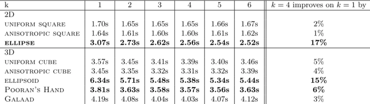
Intuitively, if the queries have some not too strong spatial coherence, the k-last-points strategy seems a good way to improve the last-point strategy. Sur-prisingly, experiments in Section 7 shows that even if the points have some strong coherence, a small k strictly greater than 1 improves on the last-point strategy when points are sorted along a space-filling curve. More precisely, k = 4 improves the location time by up to 15% on some data sets.

5 Keep, Jump & Walk

5.1 Preliminaries: Jump & Walk

The Jump & Walk technique takes a random sample of k vertices (the dots in Figure 5) of T , and uses a two-steps location process to locate a query q. First, the jump step determines the nearest vertex in the sample in (brute-force) O(k) time, then a walk in T is performed from that vertex. The usual analysis of Jump & Walk makes the hypothesis that T is the Delaunay triangulation of points evenly distributed. Taking k = n1/(d+1)_{gives a complexity of O(n}1/(d+1)₎

q

Figure 5: Jump & Walk. The walk starts from the nearest landmark (represented by dots above) with respect to the query. Then it ends at the cell containing the query.

5.2 A distribution-sensitive modification: Keep, Jump, & Walk

The classical Jump & Walk strategy [38, 23] uses a set of k landmarks randomly chosen in the vertices of T , then a query is located by walking from the closest landmark. To ensure adaptation to the query distribution instead of using vertices of T as landmarks, we keep previous queries as landmarks.Then, we have several possibilities: (i) we can use k queries chosen at random in previous queries, (ii) we can use the k last queries for the set of landmarks, and (iii) we can keep all the queries as landmarks, and regularly clear the landmarks set after a batch of k queries.

For any rule to construct the set of landmarks, the time to process a query qsplits in:

— Keep: the time K(k) for updating the set of landmarks if needed, — Jump: the time J(k) for finding the closest landmark lq, and

— Walk: the time W (k) to walk from lq to q.

This modification performs surprisingly well in practice, experimental results for method (ii) are provided in Section 7.3.

We analyze in this section the Keep, Jump, & Walk strategy. The analyses consider the straight walk as the walk strategy. We start with the following lemma, which is a fundamental piece in this section.

Lemma 12. Let T be a triangulation of n points following some distribu-tion with compact support in Rd_{, if the Distribution Condition is verified for}

a region C in the convex hull of T , then W (k) has an expected amortized O�_{F(n) · k}−1/d_{+ 1}�_{complexity for k queries.}

Proof. For k queries, the Location Tree of each variation above is an EMIT with k vertices. Let T be a triangulation of n points following some distribution with compact support in Rd_{, if the Distribution Condition is verified for a region}

S of k query points lying in C is at most κ_{· F(n) ·}�

e∈E

�e� + k = κ · F(n) · �E� + k = O�F(n) · k1−1/d+ k�. (6) Therefore, W (k) has an expected amortized O�F(n) · k−1/d_{+ 1}�_{complexity for}

kqueries.

Combining various options for F(n) and the data-structure to store the landmarks, gives us some interesting possibilities. The trick is always to balance these different costs, since increasing one decreases another.

Jump & Walk. Classical Jump & Walk uses a simple data-structure (e.g. a list) to store the random sample of T and assumes F(n) = O(n1/d_{). Here,}

we will use the same data-structure to store the set of landmarks. Keep step decides whether the query is kept at a landmark and inserts it if needed. This takes Q(k) = O(1). Jump step takes J(k) = O(k). Then, using Lemma 12 and taking k = n1/(d+1)_{landmarks amongst the queries ensures an amortized query}

time of O(n1/(d+1)_{). It is noteworthy that the complexity obtained here matches}

the classical Jump & Walk complexity with no hypotheses on the distribution of query-points (naturally, the queries must lie in the region C, which in turn must lie inside the domain of T , see Section 3).

Outside this classical framework, Jump & Walk has some interests, even with weaker hypotheses. In general considering Lemma 12, taking k = F(n)1−1/(d+1)

balances the jump and the walk costs. Another remark is that if the landmarks are a random subset of the vertices of T (as is the classical Jump & Walk), then the cost of the walk is F(n/k) [20, Variation of Lemma 4]. Assuming F(j) = O(jβ_{), the jump and the walk costs are balanced by taking k = n}1−1/(β+1) _in

this case.

Besides, if Conjecture 1 is verified, Keep, Jump, & Walk should use a sample of size k = O��n1/(d−1)�1−1/(d+1)� to construct Delaunay triangulation for points on a hypersurface, and not O(n1/(d+1)_{) as for random points in the}

space. In particular, k should be O(n3/8_{) in 3D; this is verified experimentally}

in Section 7, and should be applied in surface reconstruction applications. Walk & Walk. In Walk & Walk, the data-structure to store the landmarks is a Delaunay triangulation L, in which it is possible to walk (notice that T may not be a Delaunay triangulation). Assuming a random order on the landmarks, inserting or deleting a landmark after location takes Q(k) = O(1) and jump step takes J(k) = O(F(k)).

If the queries and the sites are both evenly distributed we get J(k) = O(k1/d₎

and, by Lemma 12, W (k) = k−1/d_{· F(n) = O(k}−1/d_{· n}1/d_{), which gives k = √n}

to balance the jump and walk costs. Finally, the point location takes expected amortized time O(n1/2d_).

If walking inside T and L takes linear time, k = n1−1/(d+1) _{balances Walk}

& Walk costs.

Delaunay Hierarchy of Queries. A natural idea is to use several layers of triangulations, walking at each level from the location at the coarser layer. When the landmarks are vertices of T and each sample takes a constant ratio of the vertices at the level below, this idea yields the Delaunay hierarchy [20].

Storing the queries in a Delaunay hierarchy may have some interesting ef-fects: If the region C of T has some bad behavior F(n) � n1/d _{and there is}

many well-distributed queries, we can get interesting query time to the price of polynomial storage. More precisely, if the queries are such that a random sample of the queries has a Delaunay triangulation of expected linear size (always true in 2D), then using a random sample of k queries for the landmarks and a De-launay hierarchy to store L, gives Q(k) = J(k) = O(log k). Then by Lemma 12 we have W (k) = O(k−1/d_{· F(n)) (amortized) and taking k = F(n)}d_{/ log}d_n

balances jump and walk costs, leading to an expected amortized logarithmic query time.

6 Climbing Up in the Delaunay Hierarchy

In this section, we show how the Delaunay hierarchy can be made distribution-sensitive under some hypotheses. Assume T is a Delaunay triangulation, then classical use of the Delaunay hierarchy provides a logarithmic cost in the total size of T to locate a point. The cost we reach here is logarithmic in the number of vertices of T in between the starting point and the query.

Given a set of n points P in the space, we assume that the expected size of the Delaunay triangulation of a random sample of size r of P has linear size. The hypothesis is always verified in 2D, and proved in several other situations: points randomly distributed in space [24] or on an hypersurface [26, 7, 8, 5]. The Delaunay hierarchy [20] constructs random samples P = P0⊆ P1⊆ P2 ⊆

. . . _{⊆ P}h such that P rob(p ∈ Pi+1| p ∈ Pi) = 1/α for some constant α > 1.

The h + 1 Delaunay triangulations Di of Pi are computed and the hierarchy is

used to find the nearest neighbor of a query q by walking at one level i from the nearest neighbor of q at the level i + 1. It is proven that the expected cost of walking at one level is O(α) and since the expected number of levels is logαn, we

obtain a logarithmic expected time to descend the hierarchy for point location.

v

0 D1 D0 D2

_v

2

q

v

1

q

q

Figure 6: Climbing. If a good starting vertex v = v0 in D0

is known, the Delau-nay hierarchy can be used in another way: From v0a walk starts

in D0 visiting

sim-plices crossed by seg-ment v0q; the walk

is stopped, either if the simplex contain-ing q is found, or if a simplex having a vertex v1 belonging

to the sample P1 is

found. If the walk

stops because v1 is

found, then a new

walk in D1 starts at v1 along segment v1q. This process continues recursively

up to the level l, where a simplex of Dl that contains q is found (see Figure 6).

Finally, the hierarchy is descended as in the usual point location. Theorem 13 bounds the complexity of this procedure.

Theorem 13. Given a set of n points P, and a convex region C ⊆ CH(P), such that the Delaunay triangulation of a random sample of size r of P

(i) has expected size O(r)

(ii) satisfies the Distribution condition in C with F(r) = rβ _{for some}

constant β,

then the expected cost of climbing and descending the Delaunay hierarchy from a vertex v to a query point q, both lying in C, is O(log w), where w is the expected cost of the walk from v to q in D the Delaunay triangulation of P.

Proof. Climbing one level. Since the probability that any vertex of Dibelongs

to Di+1 is 1/α, and that each time a new simplex is visited during the walk a

new vertex is discovered, the expected number of visited simplices before the detection of a vertex that belongs to Di+1 is 1 +�∞_j=0j_α1�1 −_α1�

j

= α. Descending one level. The cost of descending one level is O(α) [20, Lemma 4].

Number of levels. Let wi denote the number of edges crossed by viq in Di;

the Distribution Condition gives wi = F(n/αi)�viq� ≤ F(n/αi)�v0q�. If F(r)

is a polynomial function O(rβ_{), the expected number of levels that we climb}

before descending is less than l = (log w0)/β, since we have

wl= F(n/αl)�vlq� ≤ F(n/αl)�v0q� = w0/αlβ= w0/αlog w0= 1

(where the big O have been omitted). Then, at level l the walk takes constant time.

Please remind that in Section 5, we keep landmarks in order to improve the classical walking algorithm, which leads to Keep, Jump, & Walk. Now, it is nat-ural to improve the climbing algorithm described above by adding landmarks in D0 as well, and starting the climbing procedure from the nearest landmark.

Since the complexity of climbing is logarithm and not polynomial, to balance the different costs, the number of landmarks has also to be logarithmic. Such a vari-ant, called Keep, Jump, & Climb, does not improve the theoretical complexity, which remains logarithmic as for descending or climbing the Delaunay hierar-chy. However, it allows us to make the structure distribution-sensitive without penalizing that complexity. This approach will be evaluated experimentally in the next section.

7 Experimental Results

Experiments have been realized on synthetic and realistic models (scaled to fit in the unit cube). The scanned models used here: Pooran’s Hand and Galaad, are taken from the Aim@shape repository. The hardware used for the experiments described in the sequel, is a MacBook Pro 3,1 equipped with an 2.6 GHz Intel Core 2 processor and 2 GB of RAM, Mac OS X version 10.5.7. The software uses Cgal 3.6 and is compiled with g++ 4.3.2 and options O3 -DNDEBUG. All the triangulations in the experiments are Delaunay triangulations.

Each experiment was repeated 30 times, and the average is taken. The walking strategy used in the section is the stochastic walk.

We consider the following data sets in 2D: uniform square, points evenly distributed in the unit square, anisotropic square, points distributed in a

square with a ρ = x2_{density, ellipse, points evenly distributed on an ellipse;}

the lengths of the axes are 1/2, and 1. We consider the following data sets in 3D: uniform cube. Points evenly distributed in the unit cube. anisotropic cube. Points distributed in a cube with a ρ = x2_{density. ellipsoid. Points}

evenly distributed on the surface of an ellipsoid; the lengths of the ellipsoid axes are 1/3, 2/3, and 1. Pooran’s Hand. It is a data set obtained by scanning a 3D model of a hand. Galaad. It is a data set obtained by scanning a 3D model of a toy soldier.

Figure 7: Scanned models.

Files of different sizes, smaller than the original model are obtained by taking random samples of the main file with the desired number of points.

7.1 The Distribution Condition

Our first set of experiments is an experimental verification of the Distribution Condition. We compute the Delaunay triangulation of different inputs, either artificial or realistic, with several sizes; for realistic inputs we construct files of various sizes by taking random samples of the desired size.

Figure 8 shows the number of crossed tetrahedra in terms of the length of the walk, for various randomly chosen walks in the triangulation. A linear behavior with some dispersion is shown. Though, from this experiment, the walks that deviates significantly from the average behavior are more likely to be faster than slower, which is a good news.

From Figure 8, the slope of lines best fitting these point clouds give an estimation of F(n) for a particular n (namely n = 220_{). By doing these}

compu-tations for several n, we draw F(n) in terms of the triangulation size in Figure 9. If F(n) is clearly bounded by a polynomial on n, then curves in Figure 9 should be concave. Moreover, if F(n) is a polynomial on n, then curves in Figure 9 should be lines; this seems true for the ellipsoid and the cubes. Now, from the biggest slope of these different lines we evaluate the exponent of n. The points sampled on an ellipsoid give F(n) ∼ n0.52_{, which is not far from Conjecture 1}

0 0.2 0.4 0.6 0.8 1 length 0 100 200 300 400 500 600 simplices 1M points following an anisotropic ditrib. in the unit cube 0 0.2 0.4 0.6 0.8 1 length 0 200 400 600 800 1000 1200 1400 1600 simplices 1M points evenly distributed on an ellipsoid 0 0.2 0.4 0.6 0.8 1 length 0 100 200 300 400 simplices 1M points evenly distributed in a unit cube 0 0.2 0.4 0.6 0.8 1 length 0 200 400 600 800 simplices 1M points on Pooran's Hand 0 0.2 0.4 0.6 0.8 1 length 0 200 400 600 800 simplices 1M points on Galaad

Figure 8: Distribution condition. � of crossed tetrahedra in terms of the length of the walk. The number of points sampled in each model here is 220_.

F(n) ∼ n0.31_{, which is not far from F(n) = O(n}1/3_{). For the scanned models,}

the curves are a bit concave, with a slope always smaller than 0.5; the Conjec-ture 1 is also verified in these cases, since the Distribution Condition claims only an upper bound and not an exact value for the number of visited tetrahedra.

10

12

14

16

18

log n

5.5

6

6.5

7

7.5

8

8.5

log #simplices

evenly dist. unit cube

ellipsoid

Pooran's Hand

Galaad

anisotropic distrib. in the unit cube

_{log n}

Figure 9: Distribution condition. Assuming F(n) = nα_{, α is given by the}

slope of above “lines” (log here is log2).

7.2 k-last-points strategy

CGAL library [39] uses spatial sorting [17] to introduce a strong spatial co-herence in a set of points. For several models, we locate 1M queries evenly distributed inside the model with the k-last-point strategy after a spatial sort-ing of the queries. Surprissort-ingly, ussort-ing a small k slightly improves on k = 1 which indicates that even with such a strong coherence, k-last-points strategy is relevant. Table 1 shows the running times on various sets for different values of k, taking k = 4 always improves on k = 1 and in some cases by a substantial amount. k 1 2 3 4 5 6 k = 4improves on k = 1 by 2D uniform square 1.70s 1.65s 1.65s 1.65s 1.66s 1.67s 2% anisotropic square 1.64s 1.61s 1.60s 1.60s 1.61s 1.62s 1% ellipse 3.07s 2.73s 2.62s 2.56s 2.54s 2.52s 17% 3D uniform cube 3.57s 3.45s 3.41s 3.39s 3.40s 3.46s 5% anisotropic cube 3.45s 3.35s 3.32s 3.31s 3.32s 3.39s 4% ellipsoid 6.34s 5.71s 5.48s 5.38s 5.34s 5.44s 15% Pooran’s Hand 3.81s 3.63s 3.58s 3.57s 3.56s 3.63s 6% Galaad 4.19s 4.08s 4.04s 4.03s 4.07s 4.12s 3%

Table 1: Static point location with space-filling heuristic plus last-k-points strategy. Times are in seconds.

7.3 Keep, Jump, & Walk and Keep, Jump, & Climb

Now, we compare the performance of various point location procedures: clas-sical Jump & Walk (J&W), walk starting at the previous query (last-point), Keep, Jump, & Walk described in Section 5 (K&J&W), descending the Delau-nay hierarchy (classical [20]), climbing the DelauDelau-nay Hierarchy (Climb), and Keep, Jump, & Climb (K&J&C)1_{. For this purpose we consider the following}

experiment scenarios.

Scenario I — This scenario is designed to show how the proximity of queries relates to the point location algorithms performance. Let M be a scanned model with 220 _{vertices inside the unit cube, we first define S}

i, for i = 0, . . . , 20, the

2i _{vertices of M closest to the cube center. When i is large (resp. small),}

points are distributed in a large (resp. small) region on M. Then, we form the sequence Aiof 220points by taking 220times a random point from Si(repetitions

are allowed) and slightly perturbing these points. The perturbation actually removes duplicates and ensure that most of the queries are strictly inside a Delaunay tetrahedron and thus prevent many filter failures. Figure 10 shows the computation times for point location and different strategies in function of i.

Scenario II — This scenario is designed to show how the spatial coherence of queries relates with the point location algorithms performance. Imagine a scenario where N random walkers w0, w1, . . . wN−1, are walking simultaneously

with the same speed inside the unit cube containing M, and at each steps, queries are issued for each walker position. Each random walker starts at differ-ent positions and with differdiffer-ent directions. One step consists of a displacemdiffer-ent of length 0.01 for all walkers. In Figure 11, we compute the time to complete all 220 _{queries generated by 1 to 20 random walkers, for different strategies. One}

single walker means a very strong spatial coherence. Conversely, several walkers mean a weaker spatial coherence.

The walk strategy used in the experiments is the stochastic walk. To guarantee honest comparisons, we use the same stochastic walk implementation for all the experiments: the stochastic walk implemented in Cgal [48, 39].

14 15 16 17 18 19 20 sparsity 0 10 20 30 40 50 seconds last -point Delaunay hierarchy J&W, k=n1/4 K&J&W, k = n K&J&W, k = n 1/4 3/8 Climb K&J&C, k = log n 14 15 16 17 18 19 20 sparsity 0 10 20 30 40 50 seconds last-point Delaunay hierarchy J&W, k=n 1/4 K&J&W, k = n 3/8 K&J&W, k = n 1/4 Climb K&J&C, k = log n

Figure 10: Results for scenario I (proximity of queries). Computation times of the various algorithms in function of the number of points on the model enclosed by a ball centered at (0.5, 0.5, 0.5) for: (a) Pooran’s Hand model; and (b) Galaad model.

1_{All these point location strategies are also implemented in a javascript demo; we made it} available at [16].

From Scenario I. Figure 10 depicts the running time for 220 _queries.

One can observe that Keep, Jump, & Walk actually benefits from the proximity of the queries and is clearly better than Jump & Walk and even better than the Delaunay hierarchy if the portion of M where the queries lie in is below 6% of the total surface of M. Taking n3/8 _{landmarks instead of n}1/4_{performs clearly}

better which is another experimental validation of Conjecture 1 (as announced in Section 5). Not surprisingly, climbing the hierarchy is slower than descending the hierarchy when there is no locality and improves with locality. Finally, Keep, Jump, & Climb combines all the advantages and appears as the best solution in practice for this experiment.

0 5 10 15 20

number of random walkers

0 5 10 15 20 25 seconds

last-point (>1 walker around 60 secs)

Delaunay hierarchy J&W, k=n1/4 K&J&W, k = n3/8 K&J&W, k = n1/4 Climb K&J&C, k = log n 0 5 10 15 20

number of random walkers

0 5 10 15 20 25 seconds

last-point (>1 walker around 60 secs)

Delaunay hierarchy J&W, k=n1/4 K&J&W, k = n3/8 K&J&W, k = n 1/4 Climb K&J&C, k = log n

Figure 11: Results for scenario II (coherence of queries). Computation times of the various algorithms in function of the number of parallel random walkers for: (a) Pooran’s Hand model; and (b) Galaad model. Less random walkers mean strong spatial coherence (a single walker pushes that to an extreme).

From Scenario II (Figure 11). With a single walker, the spatial co-herence is very strong and we expect a very good result for the last-point strategy since it highly benefits from previous location without any overhead for maintaining any structure of any case. This is indeed what happens, but Keep, Jump, & Walk and Keep, Jump, & Climb remain quite close. And, of course, when the number of walkers increases, performance of last-point strategy fall down, while Keep, Jump, & Walk/Climb still have good running times. An interesting observation is that the Keep, Jump, & Walk with n3/8 _landmarks

does not seem to be strongly dependent on the number of walkers.

8 Conclusion

Our aim was to improve in practice the performance of point location in trian-gulation and we are mostly interested in

• queries with spatial coherence • inside 3D triangulations • in the CGAL library.

Before starting this work, our best data structure for this purpose was the Delaunay hierarchy, which can handle 1M queries in a 1M points triangulation in about 15 seconds for various scenarios. We have proposed Keep, Jump, & Climb, a new way of using the Delaunay hierarchy, which is never slower and often sig-nificantly faster than the classical descent of the Delaunay hierarchy in our ex-periments. For a reasonable amount of spatial coherence of the queries, running time are improved by a factor 2.

One of our main tool in the theoretical analysis of our work is the introduc-tion of the Distribuintroduc-tion Condiintroduc-tion that relates the expected number of tetrahe-dra intersected by a line segment with its length. It allows to analyze algorithms in a more general context than Delaunay triangulation of evenly distributed points. Our experiments shows that the Distribution Condition actually corre-sponds to some practical cases.

From a theoretical point of view, climbing the Delaunay hierarchy provides a solution to the problem of distribution-sensitive point location, which is much simpler and faster than previous data structures [32, 19], but requires some reasonable hypotheses on the point set.

As a final remark, we want to insist on the dichotomy between the straight and stochastic walk. The straight walk is used in theoretical analysis for sim-plicity and usage of previous results, while the visibility walk is used in practice since it is faster and easier to implement. Thus an interesting research direction is to get a better theoretical basis for the use of the stochastic walk.

9 Open problems

The Distribution Condition brings several questions for the computational ge-ometers. The first question is the one raised in Conjecture 1:

Question 14. Do the Delaunay triangulations of n points evenly distributed on a bounded δ-dimensional manifold embedded in the d-dimensional space behave similarly to points evenly distributed in the Euclidean space of dimension δ with respect to the Distribution Condition?

If Conjecture 1 has an affirmative answer, then walking on such triangu-lations does not depend on the ambient dimension, but only on the manifold dimension.

Figure 8 and 9 invite us to believe in a positive answer even if the points are not actually evenly distributed (they come from a laser scan), thus we may wonder what are actually the hypotheses needed by the conjecture.

Question 15. What hypotheses a sampling of a bounded δ-dimensional mani-fold embedded in the d-dimensional space should verify such that the Delaunay triangulation satisfy the Distribution Condition with F(n) = n1/δ_?

Recently Connor and Kumar [14] has been able to produce a practical point location algorithm in the plane and a k-nearest neighbor graph construction algorithm [13]. Their work relies in a well-known hypothesis called the constant factor expansion hypothesis. Let S be a finite set of n points in Rd_{, B(c, r) be}

the ball with radius r centered at c, and N Nk(q) the k-th nearest neighbor of

q. Then the constant factor expansion hypothesis requires that, for any point q lying in some region C and any k = 1, . . . , n, the number of points of S enclosed by B(q, 2 · �qN Nk(q)�) ≤ γk, where γ = O(1). The constant factor expansion

hypothesis and the Distribution Condition seem to be related, such relation will allow to translate results form points sets satifying one hypothesis to the other. Question 16. Are the Distribution Condition related, in some sense, to the constant factor expansion hypothesis?

In the plane, using the Delaunay Hierarchy of Queries, one can obtain a o(log n) distribution-sensitive point location algorithm (in expectation and amortization), as long as the triangulation scheme and distribution of points satisfy the Distribution Condition with F = o(n�_{), ∀� > 0, in the domain the}

queries lie in. Such triangulation schemes with sub-polynomial Distribution Condition seems quite restrictive but they indeed exists as shown by the exam-ple of Figure 12.

Figure 12: Fractal-like scheme. The triangulation scheme above, for points uni-formly distributed on the circle, satisfy the Distribution Condition with F = O(log n) for any closed region inside the circle. However, if we take a segment s intersecting the circle, then as n → ∞, s intersects the same number of cells regardless of its size, violating the Distribution Condition.

Question 17. What is the least restrictive set of hypotheses on the triangula-tion and on the queries, such that a o(log n) distributriangula-tion-sensitive point locatriangula-tion algorithm is possible?

Question 18. In the plane, is it possible to climb in the Delaunay Hierarchy with a good complexity and with less restrictive hypotheses than Theorem 13? Question 19. Let ∆ be any triangulation scheme (such as Delaunay, Regular, Constrained, . . .), let ρ be any distribution of points with compact support Σ ⊂ Rd_{, and let C be any region inside Σ with positive volume. For a triangulation}

T of n points following distribution ρ and built upon the triangulation scheme ∆, does the Distribution Condition necessarily hold almost everywhere in C, for some polynomial F (say F = n�d/2�_)?

Note that regions that does not satisfy the Distribution Condition exist; see Figure 12 (the circle). However, the region has no volume. We could not find an example of triangulation scheme and distribution of points, such that the Distribution Condition does not hold for some polynomial F(n), with a positive volume.

Finally, we insist one last time in the dichotomy between straight walk and stochastic walk.

Question 20. What is the actual complexity of the stochastic walk?

Acknowledgments The authors wish to thank Aim@shape for providing the re-alistic models.

References

[1] Core number library. http://cs.nyu.edu/exact/core_pages. [2] The Gnu multiple precision arithmetic library. http://gmplib.org/. [3] Leda, Library for efficient data types and algorithms.

http://www.algorithmic-solutions.com/enleda.htm.

[4] D. Aldous and J. M. Steele. Asymptotics for euclidean minimal spanning trees on random points. Probab. Theory Related Fields, 92:247–258, 1992.

[5] N. Amenta, D. Attali, and O. Devillers. Complexity of Delaunay triangulation for points on lower-dimensional polyhedra. In Proc. 18th ACM-SIAM Sympos. Discrete Algorithms, pages 1106–1113, 2007.

[6] S. Arya, T. Malamatos, and D. M. Mount. A simple entropy-based algorithm for planar point location. ACM Trans. Algorithms, 3(2):17, 2007.

[7] D. Attali and J.-Daniel Boissonnat. A linear bound on the complexity of the Delaunay triangulation of points on polyhedral surfaces. Discrete Comput. Geom., 31:369–384, 2004.

[8] D. Attali, J.-D. Boissonnat, and André Lieutier. Complexity of the Delaunay triangulation of points on surfaces: The smooth case. In Proc. 19th Annu. Symp. Comp. Geom., pages 237–246, 2003.

[9] J. Beardwood, J. H. Halton, and J. M. Hammersley. The shortest path through many points. Math. Proc. Camb. Phil. Soc., 55:299–327, 1959.

[10] P. Bose and L. Devroye. On the stabbing number of a random delaunay triangu-lation. Comput. Geom. Theory Appl., 36(2):89–105, 2007.

[11] A. Bowyer. Computing Dirichlet tesselations. Comput. J., 24:162–166, 1981. [12] CGAL Editorial Board. CGAL User and Reference Manual, 3.6 edition, 2010.

www.cgal.org.

[13] M. Connor and P. Kumar. Fast construction of k-nearest neighbor graphs for point clouds. IEEE Trans. on Visualization and Computer Graphics, 99(PrePrints), 2010.

[14] M. Connor and P. Kumar. Practical nearest neighbor search in the plane. In Proc. 9th International Symp. on Exp. Algorithms, pages 501–512, 2010.

[15] P. M. M. de Castro and O Devillers. On the size of some trees embedded in Rd_.

Research Report 7179, INRIA, 2010.

[16] Pedro Machado Manhaes de Castro and Olivier Devillers. Demo: Point Location Strategies., 2010.

http://www-sop.inria.fr/geometrica/demo/point_location_strategies/

[17] Christophe Delage. Spatial sorting. In CGAL Editorial Board, editor, CGAL User and Reference Manual. 3.6 edition, 2010.

[18] E. D. Demaine, J. S. B. Mitchell, and J. O’Rourke. The Open Problems Project. http://www.cs.smith.edu/ orourke/TOPP/.

[19] Erik D. Demaine, John Iacono, and Stefan Langerman. Proximate point search-ing. Comput. Geom. Theory Appl., 28(1):29–40, 2004.

[20] Olivier Devillers. The Delaunay hierarchy. Internat. J. Found. Comput. Sci., 13:163–180, 2002.

[21] Olivier Devillers, Sylvain Pion, and Monique Teillaud. Walking in a triangulation. Internat. J. Found. Comput. Sci., 13:181–199, 2002.

[22] Luc Devroye, Christophe Lemaire, and Jean-Michel Moreau. Expected time anal-ysis for Delaunay point location. Comput. Geom. Theory Appl., 29:61–89, 2004. [23] Luc Devroye, Ernst Peter Mücke, and Binhai Zhu. A note on point location in

Delaunay triangulations of random points. Algorithmica, 22:477–482, 1998. [24] R. Dwyer. Convex hulls of samples from spherically symmetric distributions.

Discrete Appl. Math., 31(2):113–132, 1991.

[25] J. Gao and J. M. Steele. General spacefilling curve heuristics and limit theory for the traveling salesman problem. J. Complexity, 10:230–245, 1994.

[26] Mordecai J. Golin and Hyeon-Suk Na. On the average complexity of 3d-voronoi diagrams of random points on convex polytopes. Comput. Geom. Theory Appl., 25:197–231, 2003.

[27] J. E. Goodman and J. O’Rourke, editors. Handbook of Discrete and Computa-tional Geometry. CRC Press LLC, Boca Raton, FL, 2004. 2nd edition.

[28] P. J. Green and R. R. Sibson. Computing dirichlet tessellations in the plane. Comput. J., 21:168–173, 1978.

[29] Idit Haran and Dan Halperin. An experimental study of point location in planar arrangements in cgal. J. Exp. Algorithmics, 13:2.3–2.32, 2009.

[30] John Iacono. Improved upper bounds for pairing heaps. In Proc. 7th Scandinavian Workshop on Algorithm Theor., pages 32–45, London, UK, 2000. Springer-Verlag. [31] John Iacono. Expected asymptotically optimal planar point location. Comput.

Geom. Theory Appl., 29(1):19–22, 2004.

[32] John Iacono and Stefan Langerman. Proximate planar point location. In Proc. 19th Annu. Symp. Comp. Geom., pages 220–226, 2003.

[33] Michael Kazhdan, Matthew Bolitho, and Hugues Hoppe. Poisson surface recon-struction. In Proc. 4th Eurographics Symp. on Geom. Processing, pages 61–70, Aire-la-Ville, Switzerland, Switzerland, 2006. Eurographics Association.

[34] Lutz Kettner, Kurt Mehlhorn, Sylvain Pion, Stefan Schirra, and Chee Yap. Class-room examples of robustness problems in geometric computations. In Proc. 12th European Symp. on Algorithms, volume 3221 of Lecture Notes Comput. Sci., pages 702–713. Springer-Verlag, 2004.

[35] D. G. Kirkpatrick. Optimal search in planar subdivisions. SIAM J. Comput., 12(1):28–35, 1983.

[36] D. E. Knuth. Optimum binary search trees. Acta Inf., 1:14–25, 1971.

[37] Theocharis Malamatos. Lower bounds for expected-case planar point location. Comput. Geom. Theory Appl., 39(2):91–103, 2008.

[38] Ernst P. Mücke, Isaac Saias, and Binhai Zhu. Fast randomized point location without preprocessing in two- and three-dimensional Delaunay triangulations. In Proc. 12th Annu. Sympos. Comput. Geom., pages 274–283, 1996.

[39] Sylvain Pion and Monique Teillaud. 3D triangulations. In CGAL Editorial Board, editor, CGAL User and Reference Manual. 3.6 edition, 2010.

[40] L. K. Platzman and J. J. Bartholdi, III. Spacefilling curves and the planar trav-elling salesman problem. J. ACM, 36(4):719–737, October 1989.

[41] Luis A. Santaló. Integral Geometry and Geometric Probability. Addison-Wesley, 1976.

[42] Jonathan Richard Shewchuk. Stabbing delaunay tetrahedralizations. Discrete Comput. Geom, 32:343, 2002.

[43] Steven S. Skiena. The Algorithm Design Manual. Springer, 2008.

[44] J. M. Steele. Growth rates of euclidean minimal spanning trees with power weighted edges. AnnProb, 16:1767–1787, 1988.

[45] J. M. Steele. Cost of sequential connection for points in space. Oper. Res. Lett., 8:137–142, 1989.

[46] J. M. Steele and T. L. Snyder. Worst-case growth rates of some classical problems of combinatorial optimization. SIAM J. Comput., 18:278–287, 1989.

[47] C. K. Yap and T. Dubé. The exact computation paradigm. In D.-Z. Du and F. K. Hwang, editors, Computing in Euclidean Geometry, volume 4 of Lecture Notes Series on Computing, pages 452–492. World Scientific, Singapore, 2nd edition, 1995.

[48] Mariette Yvinec. 2D triangulations. In CGAL Editorial Board, editor, CGAL User and Reference Manual. 3.6 edition, 2010.

Centre de recherche INRIA Bordeaux – Sud Ouest : Domaine Universitaire - 351, cours de la Libération - 33405 Talence Cedex Centre de recherche INRIA Grenoble – Rhône-Alpes : 655, avenue de l’Europe - 38334 Montbonnot Saint-Ismier Centre de recherche INRIA Lille – Nord Europe : Parc Scientifique de la Haute Borne - 40, avenue Halley - 59650 Villeneuve d’Ascq

Centre de recherche INRIA Nancy – Grand Est : LORIA, Technopôle de Nancy-Brabois - Campus scientifique 615, rue du Jardin Botanique - BP 101 - 54602 Villers-lès-Nancy Cedex

Centre de recherche INRIA Paris – Rocquencourt : Domaine de Voluceau - Rocquencourt - BP 105 - 78153 Le Chesnay Cedex Centre de recherche INRIA Rennes – Bretagne Atlantique : IRISA, Campus universitaire de Beaulieu - 35042 Rennes Cedex Centre de recherche INRIA Saclay – Île-de-France : Parc Orsay Université - ZAC des Vignes : 4, rue Jacques Monod - 91893 Orsay Cedex

Éditeur

INRIA - Domaine de Voluceau - Rocquencourt, BP 105 - 78153 Le Chesnay Cedex (France)