HAL Id: hal-00295828
https://hal.archives-ouvertes.fr/hal-00295828
Submitted on 26 Jan 2006
HAL is a multi-disciplinary open access
archive for the deposit and dissemination of
sci-entific research documents, whether they are
pub-lished or not. The documents may come from
teaching and research institutions in France or
abroad, or from public or private research centers.
L’archive ouverte pluridisciplinaire HAL, est
destinée au dépôt et à la diffusion de documents
scientifiques de niveau recherche, publiés ou non,
émanant des établissements d’enseignement et de
recherche français ou étrangers, des laboratoires
publics ou privés.
Technical note: Simulating chemical systems in
Fortran90 and Matlab with the Kinetic PreProcessor
KPP-2.1
A. Sandu, R. Sander
To cite this version:
A. Sandu, R. Sander. Technical note: Simulating chemical systems in Fortran90 and Matlab with the
Kinetic PreProcessor KPP-2.1. Atmospheric Chemistry and Physics, European Geosciences Union,
2006, 6 (1), pp.187-195. �hal-00295828�
www.atmos-chem-phys.org/acp/6/187/ SRef-ID: 1680-7324/acp/2006-6-187 European Geosciences Union
Chemistry
and Physics
Technical note: Simulating chemical systems in Fortran90 and
Matlab with the Kinetic PreProcessor KPP-2.1
A. Sandu1and R. Sander2
1Department of Computer Science, Virginia Polytechnic Institute and State University, Blacksburg, Virginia 24060, USA 2Air Chemistry Department, Max-Planck Institute for Chemistry, Mainz, Germany
Received: 18 July 2005 – Published in Atmos. Chem. Phys. Discuss.: 13 September 2005 Revised: 30 November 2005 – Accepted: 15 September 2005 – Published: 26 January 2006
Abstract. This paper presents the new version 2.1 of the Ki-netic PreProcessor (KPP). Taking a set of chemical reactions and their rate coefficients as input, KPP generates Fortran90, Fortran77, Matlab, or C code for the temporal integration of the kinetic system. Efficiency is obtained by carefully ex-ploiting the sparsity structures of the Jacobian and of the Hessian. A comprehensive suite of stiff numerical integra-tors is also provided. Moreover, KPP can be used to generate the tangent linear model, as well as the continuous and dis-crete adjoint models of the chemical system.
1 Introduction
Next to laboratory studies and field work, computer model-ing is one of the main methods to study atmospheric chem-istry. The simulation and analysis of comprehensive chemi-cal reaction mechanisms, parameter estimation techniques, and variational chemical data assimilation applications re-quire the development of efficient tools for the computational simulation of chemical kinetics systems. From a numerical point of view, atmospheric chemistry is challenging due to the coexistence of very stable (e.g., CH4) and very reactive
(e.g., O(1D)) species. Several software packages have been developed to integrate these stiff sets of ordinary differential equations (ODEs), e.g., Facsimile (Curtis and Sweetenham, 1987), AutoChem (http://gest.umbc.edu/AutoChem), Spack (Djouad et al., 2003), Chemkin (http://www.reactiondesign. com/products/open/chemkin.html), Odepack (http://www. llnl.gov/CASC/odepack/), and KPP (Damian et al., 1995, 2002). KPP is currently being used by many academic, re-search, and industry groups in several countries (e.g. von Glasow et al., 2002; von Kuhlmann et al., 2003; Trent-mann et al., 2003; Tang et al., 2003; Sander et al., 2005).
Correspondence to: A. Sandu
The well-established Master Chemical Mechanism (MCM, http://mcm.leeds.ac.uk/MCM/) has also recently been mod-ified to add the option of producing output in KPP syn-tax. In the present paper we focus on the new features in-troduced in the release 2.1 of KPP. These features allow an efficient simulation of chemical kinetic systems in For-tran90 and Matlab. ForFor-tran90 is the programming language of choice for the vast majority of scientific applications. Mat-lab (http://www.mathworks.com/products/matMat-lab/) provides a high-level programming environment for algorithm devel-opment, numerical computations, and data analysis and visu-alization. The Matlab code produced by KPP allows a rapid implementation and analysis of a specific chemical mech-anism. KPP-2.1 is distributed under the provisions of the GNU public license (http://www.gnu.org/copyleft/gpl.html) and can be obtained on the web at http://people.cs.vt.edu/ ∼asandu/Software/Kpp. It is also available in the electronic supplement to this paper at http://www.atmos-chem-phys. org/acp/6/187/acp-6-187-sp.zip.
The paper is organized as follows. Section 2 describes the input information necessary for a simulation, and Sect. 3 presents the output produced by KPP. Aspects of the simula-tion code generated in Fortran90, Fortran77, C, and Matlab are discussed in Sect. 4. Several applications are presented in Sect. 5. The presentation focuses on the main aspects of modeling but, in the interest of space, omits a number of important (but previously described) features. For a full description of KPP, inculding the installation procedure, the reader should consult the user manual in the electronic sup-plement.
2 Input for KPP
To create a chemistry model, KPP needs as input a chemical mechanism, a numerical integrator, and a driver. Each of these components can either be chosen from the KPP library
188 A. Sandu and R. Sander: The Kinetic PreProcessor KPP-2.1
or provided by the user. The KPP input files (with suffix .kpp) specify the model, the target language, the precision, the integrator and the driver, etc. The file name (without the suffix .kpp) serves as the default root name for the simulation. In this paper we will refer to this name as “ROOT”. To specify a KPP model, write aROOT.kpp file with the following lines:
#MODEL small_strato #LANGUAGE Fortran90 #DOUBLE ON #INTEGRATOR rosenbrock #DRIVER general #JACOBIAN SPARSE_LU_ROW #HESSIAN ON #STOICMAT ON
We now explain these elements with the help of an example.
2.1 The chemical mechanism
The KPP software is general and can be applied to any kinetic mechanism. Here, we revisit the Chapman-like stratospheric chemistry mechanism from Sandu et al. (2003) to illustrate the KPP capabilities. O2 hν →2O (R1) O + O2 →O3 (R2) O3 hν →O + O2 (R3) O + O3 →2O2 (R4) O3 hν →O(1D) + O2 (R5) O(1D) + M → O + M (R6) O(1D) + O3 →2O2 (R7) NO + O3 →NO2+O2 (R8) NO2+O → NO + O2 (R9) NO2 hν →NO + O (R10)
The#MODELcommand selects a kinetic mechanism which consists of a species file (with suffix .spc) and an equation file (with suffix .eqn). The species file lists all the species in the model. Some of them are variable (defined with#DEFVAR), meaning that their concentrations change according to the law of mass action kinetics. Others are fixed (defined with #DEFFIX), with the concentrations determined by physical and not chemical factors. For each species its atomic com-position is given (unless the user chooses to explicitly ignore it). #INCLUDE atoms #DEFVAR O = O; O1D = O; O3 = O + O + O; NO = N + O; NO2 = N + O + O; #DEFFIX M = ignore; O2 = O + O;
The chemical kinetic mechanism is specified in the KPP lan-guage in the equation file:
#EQUATIONS { Stratospheric Mechanism } <R1> O2 + hv = 2O : 2.6e-10*SUN; <R2> O + O2 = O3 : 8.0e-17; <R3> O3 + hv = O + O2 : 6.1e-04*SUN; <R4> O + O3 = 2O2 : 1.5e-15; <R5> O3 + hv = O1D + O2 : 1.0e-03*SUN; <R6> O1D + M = O + M : 7.1e-11; <R7> O1D + O3 = 2O2 : 1.2e-10; <R8> NO + O3 = NO2 + O2 : 6.0e-15; <R9> NO2 + O = NO + O2 : 1.0e-11; <R10> NO2 + hv = NO + O : 1.2e-02*SUN; Here, each line starts with an (optional) equation tag in an-gle brackets. Reactions are described as “the sum of reactants equals the sum of products” and are followed by their rate co-efficients. SUNis the normalized sunlight intensity, equal to one at noon and zero at night. The value ofSUNcan either be calculated with the KPP-generated subroutineUpdate SUN or provided by the user.
2.2 The target language and data types
The target language Fortran90 (i.e. the language of the code generated by KPP) is selected with the command:
#LANGUAGE Fortran90
Other options areFortran77,C, andMatlab. The capa-bility to generate Fortran90 and Matlab code are new features of KPP-2.1, and this is what we focus on in the current paper. The data type of the generated model is set to double pre-cision with the command:
#DOUBLE ON
2.3 The numerical integrator
The#INTEGRATORcommand specifies a numerical solver from the templates provided by KPP or implemented by the user. More exactly, it points to an integrator definition file. This file is written in the KPP language and contains a refer-ence to the integrator source code file, together with specific options required by the selected integrator.
Each integrator may require specific KPP-generated func-tions (e.g., the production/destruction function in aggregate or in split form, and the Jacobian in full or in sparse format, etc.) These options are selected through appropriate parame-ters given in the integrator definition file. Integrator-specific parameters that can be fine tuned for better performance are also included in the integrator definition file.
KPP implements several Rosenbrock methods: Ros-1 and Ros-2 (Verwer et al., 1999), Ros-3 (Sandu et al., 1997), Rodas-3 (Sandu et al., 1997), Ros-4 (Hairer and Wanner, 1991), and Rodas-4 (Hairer and Wanner, 1991). For details on Rosenbrock methods and their implementation, consult section IV.7 of Hairer and Wanner (1991).
The KPP numerical library also contains implementa-tions of several off-the-shelf, highly popular stiff numerical solvers:
– Radau5:
This Runge Kutta method of order 5 based on Radau-IIA quadrature (Hairer and Wanner, 1991) is stiffly ac-curate. The KPP implementation follows the original implementation of Hairer and Wanner (1991), and the original Fortran 77 implementation has been translated to Fortran 90 for incorporation into the KPP library. While Radau5 is relatively expensive (when compared to the Rosenbrock methods), it is more robust and is useful to obtain accurate reference solutions.
– SDIRK4:
This is an L-stable, singly-diagonally-implicit Runge Kutta method of order 4. SDIRK4 originates from Hairer and Wanner (1991), and the original Fortran 77 implementation has been translated to Fortran 90 for in-corporation into the KPP library.
– SEULEX:
This variable order stiff extrapolation code is able to produce highly accurate solutions. The KPP implemen-tation follows the one in Hairer and Wanner (1991), and the original Fortran 77 implementation has been trans-lated to Fortran 90 for incorporation into the KPP li-brary.
– LSODE, LSODES:
The Livermore ODE solver (Radhakrishnan and Hind-marsh, 1993) implements backward differentiation for-mula (BDF) methods for stiff problems. LSODE has been translated from Fortran 77 to Fortran 90 for in-corporation into the KPP library. LSODES (Radhakr-ishnan and Hindmarsh, 1993), the sparse version of the Livermore ODE solver LSODE, is modified to interface directly with the KPP generated code.
– VODE:
This solver (Brown et al., 1989) uses a different formu-lation of backward differentiation formulas. The ver-sion of VODE present in the KPP library uses directly the KPP sparse linear algebra routines.
– ODESSA:
The BDF-based direct-decoupled sensitivity integrator ODESSA (Leis and Kramer, 1986) has been modified to use the KPP sparse linear algebra routines.
All methods in the KPP library have excellent stability prop-erties for stiff systems. The computational work per time step depends on the type of method (BDF, Runge Kutta, or Rosen-brock). For Rosenbrock methods it increases with the num-ber of stages. The order of accuracy typically increases with the number of stages as well. For example, Ros-2 uses only two stages and is an order 2 method while Ros-4 has 4 stages and is an order 4 method. Despite their added work, higher order methods are typically more efficient when higher ac-curacy is desired. The KPP library offers different methods that can have relative advantages depending on the level of desired solution accuracy. Regarding stability, all the Rosen-brock methods are L-stable, and therefore are well suited for stiff problems. For these methods the embedded formulas are also L-stable (or strongly A-stable) which makes the step size controller work well for stiff problems. Radau5 is a fully implicit Runge Kutta method with 3 stages and order 5. Each step is relatively expensive since it requires one real and one complex LU decomposition. However, Radau5 is very ro-bust and can provide solutions of high accuracy. It is rec-ommended that Radau5 is used to obtain reference solutions, against which one can check the correctness and the accuracy of other methods. A lighter (less expensive) Runge Kutta method is SDIRK4, a diagonally implicit formula of order 4, which only requires one real LU decomposition per step (SDIRK4 has about the same cost as a Rosenbrock method, but it performs some additional back substitutions required in the solution of nonlinear systems at each step). While SDIRK4 does not have the strong nonlinear stability prop-erties of Radau5, it is L-stable and is also well suited for solving stiff chemical kinetics.
The implementations use the KPP sparse linear algebra routines by default. However, full linear algebra (using LA-PACK routines) is also implemented. To switch from sparse to full linear algebra the user only needs to define the prepro-cessor variable (-DFULL ALGEBRA=1) during compilation.
2.4 The driver
The so-called driver is the main program. It is responsible for calling the integrator routine, reading the data from files and writing the results. Existing drivers differ from one another by their input and output data file format, and by the auxil-iary files created for interfacing with visualization tools. For large 3-D atmospheric chemistry simulations, the 3-D code will replace the default drivers and call the KPP-generated routines directly. In our current implementation of KPP into a 3-D model (Sander et al., 2005), the chemical mechanism is integrated separately for each grid cell. The interaction be-tween the grid cells (advection, diffusion, convection . . . ) is calculated outside of KPP, i.e. the operator splitting approach is used.
190 A. Sandu and R. Sander: The Kinetic PreProcessor KPP-2.1
2.5 The substitution preprocessor
Templates are inserted into the simulation code after be-ing run by the substitution preprocessor. This preprocessor replaces placeholders in the template files with their partic-ular values in the model at hand. For example,KPP ROOT is replaced by the model (ROOT) name, KPP REAL by the selected real data type, andKPP NSPECandKPP NREACT by the numbers of species and reactions, respectively.
2.6 The inlined code
In order to offer maximum flexibility, KPP allows the user to include pieces of code in the kinetic description file. Inlined code begins on a new line with#INLINEand the inline type. Next, one or more lines of code follow, written in Fortran90, Fortran77, C, or Matlab, as specified by the inline type. The inlined code ends with#ENDINLINE. The code is inserted into the KPP output at a position which is also determined by inline type.
3 Output of KPP
KPP generates code for the temporal integration of chemical systems. This code consists of a set of global variables, plus several functions and subroutines. The code distinguishes between variable and fixed species. The ordinary differential equations are produced for the time evolution of the vari-able species. Fixed species enter the chemical reactions, but their concentrations are not modified. For example, the at-mospheric oxygen O2is reactive, however its concentration
is in practice not influenced by chemical reactions.
3.1 Parameters
KPP defines a complete set of simulation parameters which are global and can be accessed by all functions. Im-portant simulation parameters are the total number of species (NSPEC=7), the number of variable (NVAR=5) and fixed (NFIX=2) species, the number of chemical reactions (NREACT=10), the number of nonzero entries in the Jaco-bian (NONZERO=18) and in the sparse Hessian (NHESS=10), etc. The explicit values given here refer to our example from Sect. 2.1. KPP orders the variable species such that the spar-sity pattern of the Jacobian is maintained after an LU decom-position and defines their indices explicitly. For our example:
ind_O1D=1, ind_O=2, ind_O3=3, ind_NO=4, ind_NO2=5, ind_M=6, ind_O2=7
3.2 Global data
KPP defines a set of global variables that can be accessed by all routines. This set includesC(NSPEC), the array of con-centrations of all species.Ccontains variable (VAR(NVAR)) and fixed (FIX(NFIX)) species. Rate coefficients are
stored inRCONST(NREACT), the current integration time is TIME, absolute and relative integration tolerances are ATOL(NSPEC)andRTOL(NSPEC), etc.
3.3 The chemical ODE function
The chemical ODE system for our example is:
d [O(1D)] dt =k5[O3]−k6[O( 1D)] [M]−k 7[O(1D)] [O3] d [O] dt =2 k1[O2]−k2[O] [O2] +k3[O3] −k4[O] [O3] +k6[O(1D)] [M] −k9[O] [NO2] +k10[NO2] d [O3] dt =k2[O] [O2]−k3[O3]−k4[O] [O3]−k5[O3] −k7[O(1D)] [O3]−k8[O3] [NO] d [NO] dt = −k8[O3] [NO] + k9[O] [NO2] +k10[NO2] d [NO2] dt =k8[O3] [NO]−k9[O] [NO2]−k10[NO2] where square brackets denote concentrations of the species. The chemical ODE system has dimensionNVAR. The con-centrations of fixed species are parameters in the derivative function. KPP computes the vectorAof reaction rates and the vectorVdot of variable species time derivatives. The input argumentsVandFare the concentrations of variable and fixed species, respectively. RCTcontains the rate coeffi-cients. Below is the Fortran90 code generated by KPP for the ODE function of our example stratospheric system. It shows how the KPP-generated code forVdotcorresponds to the ODE system shown above, using the indicies from Sect. 3.1:
SUBROUTINE Fun (V, F, RCT, Vdot ) USE small_Precision
USE small_Params
REAL(kind=DP) :: V(NVAR), & F(NFIX), RCT(NREACT), & Vdot(NVAR), A(NREACT) & ! Computation of equation rates
A(1) = RCT(1)*F(2) A(2) = RCT(2)*V(2)*F(2) A(3) = RCT(3)*V(3) A(4) = RCT(4)*V(2)*V(3) A(5) = RCT(5)*V(3) A(6) = RCT(6)*V(1)*F(1) A(7) = RCT(7)*V(1)*V(3) A(8) = RCT(8)*V(3)*V(4) A(9) = RCT(9)*V(2)*V(5) A(10) = RCT(10)*V(5) ! Aggregate function Vdot(1) = A(5)-A(6)-A(7) Vdot(2) = 2*A(1)-A(2)+A(3) &
-A(4)+A(6)-A(9)+A(10)
Vdot(3) = A(2)-A(3)-A(4)-A(5) & -A(7)-A(8)
Vdot(4) = -A(8)+A(9)+A(10) Vdot(5) = A(8)-A(9)-A(10) END SUBROUTINE Fun
3.4 The chemical ODE Jacobian
The Jacobian matrix for our example contains 18 non-zero elements: J(1, 1) = −k6[M]−k7[O3] J(1, 3) = k5−k7[O(1D)] J(2, 1) = k6[M] J(2, 2) = −k2[O2]−k4[O3]−k9[NO2] J(2, 3) = k3−k4[O] J(2, 5) = −k9[O] + k10 J(3, 1) = −k7[O3] J(3, 2) = k2[O2]−k4[O3] J(3, 3) = −k3−k4[O]−k5−k7[O(1D)]−k8[NO] J(3, 4) = −k8[O3] J(4, 2) = k9[NO2] J(4, 3) = −k8[NO] J(4, 4) = −k8[O3] J(4, 5) = k9[O] + k10 J(5, 2) = −k9[NO2] J(5, 3) = k8[NO] J(5, 4) = k8[O3] J(5, 5) = −k9[O]−k10
It defines how the temporal change of each chemical species depends on all other species. For example, J(5, 2) shows that NO2(species number 5) is affected by O (species number 2)
via reaction number R9.
The command #JACOBIAN controls the generation of the Jacobian routine. The option OFF inhibits the con-struction of the Jacobian. The optionFULL generates the subroutineJac(V,F,RCT,JVS)which produces a square (NVAR×NVAR) Jacobian.
The options SPARSE ROW and SPARSE LU ROW gen-erate the routine Jac SP(V,F,RCT,JVS) which pro-duces the Jacobian in sparse (compressed on rows) for-mat. With the option SPARSE LU ROW, KPP extends the number of nonzeros to account for the fill-in due to the LU decomposition. The vector JVS contains the LU NONZERO elements of the Jacobian in row or-der. Each row I starts at position LU CROW(I), and LU CROW(NVAR+1)=LU NONZERO+1. The location of theI-th diagonal element is LU DIAG(I). The sparse el-ementJVS(K)is the Jacobian entry in rowLU IROW(K)
and columnLU ICOL(K). The sparsity coordinate vectors are computed by KPP and initialized statically. These vec-tors are constant as the sparsity pattern of the Hessian does not change during the computation.
The routines Jac SP Vec(JVS,U,V) and JacTR SP Vec(JVS,U,V) perform sparse multipli-cation ofJVS(or its transpose) with a user-supplied vector Uwithout any indirect addressing.
3.5 Sparse linear algebra
To numerically solve for the chemical concentrations one must employ an implicit timestepping technique, as the sys-tem is usually stiff. Implicit integrators solve syssys-tems of the form
P x = (I − hγ J) x = b (1)
where the matrix P=I−hγ J is refered to as the “prediction matrix”. I the identity matrix, h the integration time step, γ a scalar parameter depending on the method, and J the system Jacobian. The vector b is the system right hand side and the solution x typically represents an increment to update the solution.
The chemical Jacobians are typically sparse, i.e. only a relatively small number of entries are nonzero. The sparsity structure of P is given by the sparsity structure of the Jaco-bian, and is produced by KPP with account for the fill-in. By carefully exploiting the sparsity structure, the cost of solving the linear system can be considerably reduced.
KPP orders the variable species such that the sparsity pat-tern of the Jacobian is maintained after an LU decomposition. KPP defines a complete set of simulation parameters, includ-ing the numbers of variable and fixed species, the number of chemical reactions, the number of nonzero entries in the sparse Jacobian and in the sparse Hessian, etc.
KPP generates the routineKppDecomp(P,IER)which performs an in-place, non-pivoting, sparse LU decomposi-tion of the matrix P. Since the sparsity structure accounts for fill-in, all elements of the full LU decomposition are actually stored. The output argument IER returns a nonzero value if singularity is detected.
The routines KppSolve(P,b,x) and KppSolveTR(P,b,x) use the LU factorization of P as computed byKppDecompand perform sparse backward and forward substitutions to solve the linear systems P x=b and PT x=b, respectively. The KPP sparse linear algebra
routines are extremely efficient, as shown in Sandu et al. (1996).
3.6 The chemical ODE Hessian
The Hessian is used for sensitivity analysis calculations. It contains second order derivatives of the time derivative
func-192 A. Sandu and R. Sander: The Kinetic PreProcessor KPP-2.1
tions. More exactly, the Hessian is a 3-tensor such that
HESSi,j,k=
∂2(Vdot)i
∂Vj∂Vk
, 1 ≤ i, j, k ≤NVAR. (2)
With the command #HESSIAN ON, KPP produces the routineHessian(V,F,RCT,HESS)which calculates the HessianHESSusing the variable (V) and fixed (F) concen-trations, and the rate coefficients (RCT).
The Hessian is a very sparse tensor. KPP computes the number of nonzero Hessian entries (and saves this in the variableNHESS). The Hessian itself is represented in coor-dinate sparse format. The real vectorHESSholds the values, and the integer vectorsIHESS I,IHESS J, andIHESS K hold the indices of nonzero entries. Since the time derivative function is smooth, these Hessian matrices are symmetric, HESS(I,J,K)=HESS(I,K,J). KPP generates code only for those entriesHESS(I,J,K)withJ≤K.
The sparsity coordinate vectorsIHESS I,IHESS J, and IHESS K are computed by KPP and initialized statically. These vectors are constant as the sparsity pattern of the Hes-sian does not change during the simulation.
The routines Hess Vec(HESS,U1,U2,HU) and HessTR Vec(HESS,U1,U2,HU) compute the action of the Hessian (or its transpose) on a pair of user-supplied vectorsU1,U2. Sparse operations are employed to produce the result vectorHU.
3.7 Utility routines
In addition to the chemical system description routines dis-cussed above, KPP generates several utility routines. They are used to set initial values and to update the rate coeffi-cients, e.g. according to current temperature, pressure, and solar zenith angle.
It was shown in Sect. 2.1 that each reaction may contain an equation tag. KPP can generate code that allows to ob-tain individual reaction rates as well as a string describing the chemical reaction. This information could be used, for example, to analyze the chemical mechanism and identify important reaction cycles as shown by Lehmann (2004).
4 Language-specific code generation
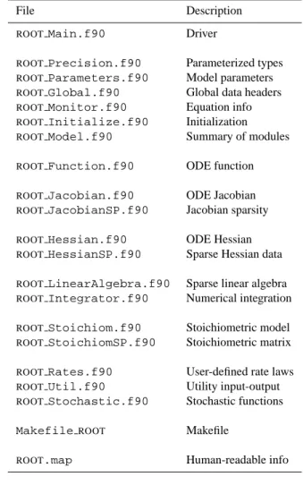
The code generated by KPP for the kinetic model description is organized in a set of separate files. The files associated with the modelROOTare named with the prefix “ROOT”. A list of KPP-generated files is shown in Table 1.
4.1 Fortran90
The generated code is consistent with the Fortran90 standard. It will not exceed the maximum number of 39 continuation lines. If KPP cannot properly split an expression to keep the number of continuation lines below the threshold then it will
Table 1. List of KPP-generated files (for Fortran90).
File Description
ROOT Main.f90 Driver
ROOT Precision.f90 Parameterized types
ROOT Parameters.f90 Model parameters
ROOT Global.f90 Global data headers
ROOT Monitor.f90 Equation info
ROOT Initialize.f90 Initialization
ROOT Model.f90 Summary of modules
ROOT Function.f90 ODE function
ROOT Jacobian.f90 ODE Jacobian
ROOT JacobianSP.f90 Jacobian sparsity
ROOT Hessian.f90 ODE Hessian
ROOT HessianSP.f90 Sparse Hessian data
ROOT LinearAlgebra.f90 Sparse linear algebra
ROOT Integrator.f90 Numerical integration
ROOT Stoichiom.f90 Stoichiometric model
ROOT StoichiomSP.f90 Stoichiometric matrix
ROOT Rates.f90 User-defined rate laws
ROOT Util.f90 Utility input-output
ROOT Stochastic.f90 Stochastic functions
MakefileROOT Makefile
ROOT.map Human-readable info
generate a warning message pointing to the location of this expression.
The driver fileROOT Main.f90contains the main For-tran90 program. All other code is enclosed in Fortran mod-ules. There is exactly one module in each file, and the name of the module is identical to the file name but without the suffix.f90.
Fortran90 code uses parameterized real types. KPP gener-ates the moduleROOT Precisionwhich contains the sin-gle and double real kind definitions:
INTEGER, PARAMETER :: &
SP = SELECTED_REAL_KIND(6,30), & DP = SELECTED_REAL_KIND(12,300) Depending on the user choice of the #DOUBLEswitch the real variables are of type double or single precision. Chang-ing the parameters of theSELECTED REAL KINDfunction in this module will cause a change in the working precision for the whole model.
The global parameters (Sect. 3.1) are defined and initial-ized in the moduleROOT Parameters. The global vari-ables (Sect. 3.2) are declared in the moduleROOT Global. They can be accessed from within each program unit that uses the global module.
The sparse data structures for the Jacobian (Sect. 3.4) are declared and initialized in the moduleROOT JacobianSP. The sparse data structures for the Hessian (Sect. 3.6) are de-clared and initialized in the moduleROOT HessianSP.
The code for the ODE function (Sect. 3.3) is in mod-ule ROOTFunction. The code for the ODE Jaco-bian and sparse multiplications (Sect. 3.4) is in mod-ule ROOTJacobian. The Hessian function and as-sociated sparse multiplications (Sect. 3.6) are in module
ROOT Hessian.
The module ROOTStoichiom contains the functions for reactant products and its Jacobian, and derivatives with respect to rate coefficients. The declaration and initialization of the stoichiometric matrix and the associated sparse data structures is done in the moduleROOT StoichiomSP.
Sparse linear algebra routines (Sect. 3.5) are in the mod-uleROOT LinearAlgebra. The code to update the rate constants and the user defined rate law functions are in mod-ule ROOTRates. The utility and input/output functions (Sect. 3.7) are inROOT UtilandROOTMonitor.
Matlab-mex gateway routines for the ODE function, Jaco-bian, and Hessian are discussed in Sect. 4.5.
4.2 Matlab
Matlab code allows for rapid prototyping of chemical kinetic schemes, and for a convenient analysis and visualization of the results. Differences between different kinetic mecha-nisms can be easily understood. The Matlab code can be used to derive reference numerical solutions, which are then compared against the results obtained with user-supplied nu-merical techniques. Last but not least Matlab is an excellent environment for educational purposes. KPP/Matlab can be used to teach students fundamentals of chemical kinetics and chemical numerical simulations.
Each Matlab function has to reside in a separate m-file. Function calls use the m-function-file names to reference the function. Consequently, KPP generates one m-function-file for each of the functions discussed in Sects. 3.3, 3.4, 3.5, 3.6, and 3.7. The names of the m-function-files are the same as the names of the functions (prefixed by the model name
ROOT).
The global parameters (Sect. 3.1) are defined as Matlab global variables and initialized in the file
ROOT parameter defs.m. The global variables (Sect. 3.2) are declared as Matlabglobalvariables in the file ROOTGlobal defs.m. They can be accessed from within each Matlab function by usingglobaldeclarations of the variables of interest.
The sparse data structures for the Jacobian (Sect. 3.4), the Hessian (Sect. 3.6), the stoichiometric matrix and the Jaco-bian of reaction products are declared as Matlab global variables in the fileROOT Sparse defs.m. They are ini-tialized in separate m-files, namelyROOT JacobianSP.m
ROOT HessianSP.m, and ROOTStoichiomSP.m, re-spectively.
Two wrappers (ROOT Fun Chem.m and
ROOT Jac SP Chem.m) are provided for interfacing the ODE function and the sparse ODE Jacobian with Matlab’s suite of ODE integrators. Specifically, the syntax of the wrapper calls matches the syntax required by Matlab’s integrators like ode15s. Moreover, the Jacobian wrapper converts the sparse KPP format into a Matlab sparse matrix.
4.3 C
The driver fileROOT Main.ccontains the main driver and numerical integrator functions, as well as declarations and initializations of global variables (Sect. 3.2).
The generated C code includes three header files which are #include-d in other files as appropriate. The global parameters (Sect. 3.1) are #define-d in the header file
ROOT Parameters.h. The global variables (Sect. 3.2) are extern-declared in ROOT Global.h, and declared in the driver fileROOT.c. The header fileROOT Sparse.h contains extern declarations of sparse data structures for the Jacobian (Sect. 3.4), Hessian (Sect. 3.6), stoichiometric ma-trix and the Jacobian of reaction products. The actual decla-rations of each data structures is done in the corresponding files.
The code for each of the model functions, integration rou-tine, etc. is located in the corresponding file (with extension .c) as shown in Table 1.
Finally, Matlab mex gateway routines that allow the C im-plementation of the ODE function, Jacobian, and Hessian to be called directly from Matlab (Sect. 4.5) are also generated.
4.4 Fortran77
The general layout of the Fortran77 code is similar to the layout of the C code. The driver fileROOTMain.fcontains the main program and the initialization of global variables.
The generated Fortran77 code includes three header files. The global parameters (Sect. 3.1) are de-fined as parameters and initialized in the header file
ROOT Parameters.h. The global variables (Sect. 3.2) are declared in ROOT Global.h as common block vari-ables. There are global common blocks for real (GDATA), integer (INTGDATA), and character (CHARGDATA) global data. They can be accessed from within each program unit that includes the global header file.
The header fileROOT Sparse.hcontains common block declarations of sparse data structures for the Jacobian (Sect. 3.4), Hessian (Sect. 3.6), stoichiometric matrix and the
194 A. Sandu and R. Sander: The Kinetic PreProcessor KPP-2.1
Jacobian of reaction products. These sparse data structures are initialized in four named “block data” statements.
The code for each of the model functions, integration rou-tine, etc. is located in the corresponding file (with extension .f) as shown in Table 1.
Matlab-mex gateway routines for the ODE function, Jaco-bian, and Hessian are discussed in Sect. 4.5.
4.5 Mex interfaces
KPP generates mex gateway routines for the ODE func-tion (ROOT mex Fun), Jacobian (ROOT mex Jac SP), and Hessian (ROOT mex Hessian), for the target languages C, Fortran77, and Fortran90.
After compilation (using Matlab’s mex compiler) the mex functions can be called instead of the corresponding Mat-lab m-functions. Since the calling syntaxes are identical, the user only has to insert the “mex” string within the cor-responding function name. Replacing m-functions by mex-functions gives the same numerical results, but the computa-tional time could be considerably shorter, especially for large kinetic mechanisms.
If possible we recommend to build mex files using the C language, as Matlab offers most mex interface options for the C language. Moreover, Matlab distributions come with a native C compiler (lcc) for building executable functions from mex files. Fortran77 mex files work well on most plat-forms without additional efforts. The mex files built using Fortran90 may require further platform-specific tuning of the mex compiler options.
5 Applications
In this section we illustrate several applications using KPP.
5.1 Benchmark tests
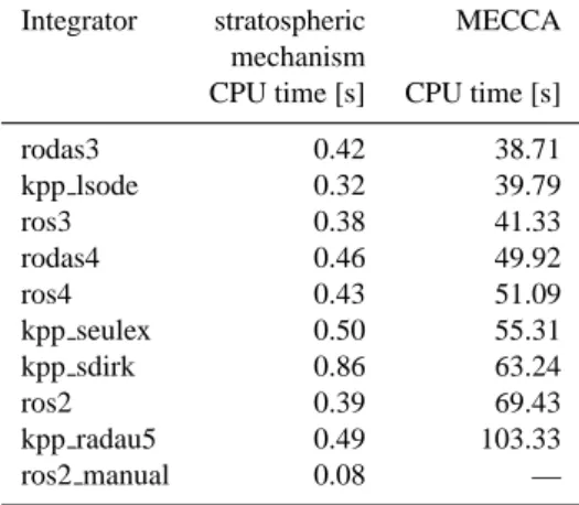
We performed some model runs to test the stability and ef-ficiency of the KPP integrators. First, we used the very simple Chapman-like stratospheric mechanism. Simulations of one month were made using the 10 different integrators ros2, ros3, ros4, rodas3, rodas4, ros2 manual, kpp radau5, kpp sdirk, kpp seulex, and kpp lsode. The CPU times used for the runs are shown in Table 2. Radau5, the most ac-curate integrator, is also the slowest. Since the overhead for the automatic time step control is relatively large in this small mechanism, the integrator ros2 manual with manual time step control is by far the fastest here. However, it is also the least precise integrator, when compared to Radau5 as reference.
As a second example, we have performed runs with the complex chemistry model MECCA (Sander et al. (2005), see also http://www.mpch-mainz.mpg.de/∼sander/ messy/mecca/) simulating gas and aerosol chemistry in the marine boundary layer. We have selected a subset of the
Table 2. Benchmark tests with the small stratospheric mechanism
and with MECCA performed on on a Linux PC with a 2 GHz CPU.
Integrator stratospheric MECCA mechanism
CPU time [s] CPU time [s] rodas3 0.42 38.71 kpp lsode 0.32 39.79 ros3 0.38 41.33 rodas4 0.46 49.92 ros4 0.43 51.09 kpp seulex 0.50 55.31 kpp sdirk 0.86 63.24 ros2 0.39 69.43 kpp radau5 0.49 103.33 ros2 manual 0.08 —
MECCA mechanism with 212 species, 106 gas-phase tions, 266 aqueous-phase reactions, 154 heterogeneous reac-tions, 37 photolyses, and 48 aqueous-phase equilibria. The CPU times for 8-day simulations with different integrators are shown in Table 2. Again, Radau5 is the slowest in-tegrator. The Rosenbrock integrators with automatic time step control and LSODE are much faster. The integrator ros2 manual with manual time step control was unable to solve this very stiff system of differential equations.
5.2 Direct and adjoined sensitivity studies
KPP has recently been extended with the capability to gen-erate code for direct and adjoint sensitivity analysis. This was described in detail by Sandu et al. (2003) and Daescu et al. (2003). Here, we only briefly summarize these features. The direct decoupled method, build using backward differ-ence formulas (BDF), has been the method of choice for di-rect sensitivity studies. The didi-rect decoupled approach was extended to Rosenbrock stiff integration methods. The need for Jacobian derivatives prevented Rosenbrock methods to be used extensively in direct sensitivity calculations. However, the new automatic differentiation and symbolic differentia-tion technologies make the computadifferentia-tion of these derivatives feasible. The adjoint modeling is an efficient tool to evalu-ate the sensitivity of a scalar response function with respect to the initial conditions and model parameters. In addition, sensitivity with respect to time dependent model parameters may be obtained through a single backward integration of the adjoint model. KPP software may be used to completely generate the continuous and discrete adjoint models taking full advantage of the sparsity of the chemical mechanism. Flexible direct-decoupled and adjoint sensitivity code imple-mentations are achieved with minimal user intervention.
6 Conclusions
The widely-used software environment KPP for the simula-tion of chemical kinetics was added the capabilities to gen-erate simulation code in Fortran90 and Matlab. An update of the Fortran77 and C generated code was also performed. The new capabilities will allow researchers to include KPP generated modules in state-of-the-art large scale models, for example in the field of air quality studies. Many of these models are implemented in Fortran90. The Matlab capabil-ities will allow for a rapid prototyping of chemical kinetic systems, and for the visualization of the results. Matlab also offers an ideal educational environment and KPP can be used in this context to teach introductory chemistry or modeling classes.
The KPP-2.1 source code is distributed under the pro-visions of the GNU public license (http://www.gnu.org/ copyleft/gpl.html) and is available in the electronic supple-ment to this paper at http://www.atmos-chem-phys.org/acp/ 6/187/acp-6-187-sp.zip. The source code and the docu-mentation can also be obtained from http://people.cs.vt.edu/ ∼asandu/Software/Kpp.
Acknowledgements. The work of A. Sandu was supported by the awards NSF-CAREER ACI 0413872 and NSF-ITR AP&IM 0205198.
Edited by: M. Ammann
References
Brown, P., Byrne, G., and Hindmarsh, A.: VODE: A Variable Step ODE Solver, SIAM J. Sci. Stat. Comput., 10, 1038–1051, 1989. Curtis, A. R. and Sweetenham, W. P.: Facsimile/Chekmat User’s Manual, Tech. rep., Computer Science and Systems Division, Harwell Lab., Oxfordshire, Great Britain, 1987.
Daescu, D., Sandu, A., and Carmichael, G. R.: Direct and ad-joint sensitivity analysis of chemical kinetic systems with KPP: II – Validation and numerical experiments, Atmos. Environ., 37, 5097–5114, 2003.
Damian, V., Sandu, A., Damian, M., Carmichael, G. R., and Potra, F. A.: KPP – A symbolic preprocessor for chemistry kinetics – User’s guide, Technical report, The University of Iowa, Iowa City, IA 52246, 1995.
Damian, V., Sandu, A., Damian, M., Potra, F., and Carmichael, G. R.: The kinetic preprocessor KPP – a software environment for solving chemical kinetics, Comput. Chem. Eng., 26, 1567– 1579, 2002.
Djouad, R., Sportisse, B., and Audiffren, N.: Reduction of mul-tiphase atmospheric chemistry, J. Atmos. Chem., 46, 131–157, 2003.
Hairer, E. and Wanner, G.: Solving Ordinary Differential Equations II. Stiff and Differential-Algebraic Problems, Springer-Verlag, Berlin, 1991.
Lehmann, R.: An algorithm for the determination of all significant pathways in chemical reaction systems, J. Atmos. Chem., 47, 45–78, 2004.
Leis, J. and Kramer, M.: ODESSA – An Ordinary Differential Equation Solver with Explicit Simultaneous Sensitivity Analy-sis, ACM Transactions on Mathematical Software, 14, 61–67, 1986.
Radhakrishnan, K. and Hindmarsh, A.: Description and use of LSODE, the Livermore solver for differential equations, NASA reference publication 1327, 1993.
Sander, R., Kerkweg, A., J¨ockel, P., and Lelieveld, J.: Technical Note: The new comprehensive atmospheric chemistry module MECCA, Atmos. Chem. Phys., 5, 445–450, 2005,
SRef-ID: 1680-7324/acp/2005-5-445.
Sandu, A., Potra, F. A., Damian, V., and Carmichael, G. R.: Effi-cient implementation of fully implicit methods for atmospheric chemistry, J. Comp. Phys., 129, 101–110, 1996.
Sandu, A., Verwer, J. G., Blom, J. G., Spee, E. J., Carmichael, G. R., and Potra, F. A.: Benchmarking stiff ODE solvers for at-mospheric chemistry problems II: Rosenbrock solvers, Atmos. Environ., 31, 3459–3472, 1997.
Sandu, A., Daescu, D., and Carmichael, G. R.: Direct and adjoint sensitivity analysis of chemical kinetic systems with KPP: I – Theory and software tools, Atmos. Environ., 37, 5083–5096, 2003.
Tang, Y., Carmichael, G. R., Uno, I., Woo, J.-H., Kurata, G., Lefer, B., Shetter, R. E., Huang, H., Anderson, B. E., Avery, M. A., Clarke, A. D., and Blake, D. R.: Impacts of aerosols and clouds on photolysis frequencies and photochemistry during TRACE-P: 2. Three-dimensional study using a regional chemical transport model, J. Geophys. Res., 108D, doi:10.1029/2002JD003100, 2003.
Trentmann, J., Andreae, M. O., and Graf, H.-F.: Chemical processes in a young biomass-burning plume, J. Geophys. Res., 108D, doi: 10.1029/2003JD003732, 2003.
Verwer, J., Spee, E., Blom, J. G., and Hunsdorfer, W.: A second order Rosenbrock method applied to photochemical dispersion problems, SIAM Journal on Scientific Computing, 20, 1456– 1480, 1999.
von Glasow, R., Sander, R., Bott, A., and Crutzen, P. J.: Modeling halogen chemistry in the marine boundary layer. 1. Cloud-free MBL, J. Geophys. Res., 107D, 4341, doi:10.1029/ 2001JD000942, 2002.
von Kuhlmann, R., Lawrence, M. G., Crutzen, P. J., and Rasch, P. J.: A model for studies of tropospheric ozone and nonmethane hydrocarbons: Model description and ozone results, J. Geophys. Res., 108D, doi:10.1029/2002JD002893, 2003.