Baiting for defense against stealthy attacks on cyber-physical systems

Baiting For Defense Against Stealthy Attacks on

Cyber-Physical Systems

by

David B. Flamholz

Bachelor of Science, Massachusetts Institute of Technology (2015)

Submitted to the Department of Mechanical Engineering

in partial fulfillment of the requirements for the degree of

Master of Science in Mechanical Engineering

at the

MASSACHUSETTS INSTITUTE OF TECHNOLOGY

February 2019

@

Massachusetts Institute of Technology 2019. All rights reserved.

Auho.Signature

redacted

Author .

S i n t r

e a t d

...

Department of Mechanical Engineering

January 15, 2019

Certified by...

Accepted by...

MASSACHUS S INSTITUTE OF TECHNOLOGY

FEB 252019

LIBRARIES

Signature redacted

Anuradha M. Annaswamy

Senior Research Scientist

Thesis Supervisor

Signature redacted

Niclas Hadjiconstantinou

Chairman, Department Committee on Graduate Students

Baiting For Defense Against Stealthy Attacks on

Cyber-Physical Systems

by

David B. Flamholz

Submitted to the Department of Mechanical Engineering on January 15, 2019, in partial fulfillment of the

requirements for the degree of

Master of Science in Mechanical Engineering

Abstract

The goal of this thesis is to develop a defense methodology for a cyber-physical system (CPS) by which an attempted stealthy cyber-attack is detected in near real time. Improvements in networked communication have enabled vast and complex dynamic control systems to exploit networked control schemes to seamlessly integrate parts and processes. These cyber-physical systems exhibit a level of flexibility that was previously unavailable but also introduce communication channels that are vulnerable to outside interference and malicious intervention.

This thesis considers the effects of a type of stealthy attack on a class of CPS that can be modeled as linear time-invariant systems. The effects of this attack are studied from both the perspective of the attacker as well as the defender. A previously developed method for conducting stealthy attacks is introduced and analyzed. This method consists of injecting malicious actuation signals into the control input of a CPS and then designing a sensor attack to conceal the effect of the actuator attack. The result is an attack that cannot be detected upon inspection of the Kalman filter residual. Successful implementation of this attack is shown to require the attacker to attain perfect model knowledge in order for the attack to be stealthy.

Based on the execution of past attacks on CPS, this thesis proposes an attacker who starts their attack by "fishing" for critical and confidential system information such as the model parameters. A method is then proposed in which the defender attempts to feed the attacker a slightly falsified model, baiting the fishing attacker

with data that will make an attack detectable. Because the attacker's model is

no longer correct, their attack design will induce a mean-shift in the Kalman filter residual, breaking the stealthiness of the original attack formula. It is then shown that the defender can not only detect this faulty attack, but use observations of the Kalman filter residual to regain more accurate state estimates, mitigating the effect of the attack.

Thesis Supervisor: Anuradha M. Annaswamy Title: Senior Research Scientist

Acknowledgments

I would like to thank my advisor, Dr. Anuradha Annaswamy for her guidance and support throughout my research process and for teaching me new tools and ways of thinking along the way. I appreciate the time she has taken to smooth my transition into academic research and help me reason out how to handle the challenges I faced. I would like to thank Dr. Eugene Lavretsky for his advice and support along with the support of the Boeing Strategic University Initiative.

I owe special thanks to a number of friends and colleagues who supported me throughout this process and spent many hours listening to me practice presentations, helping me understand tough concepts, and helping me de-bug problems with my simulations. I would like to extend special thanks to my colleagues in the Active Adaptive Control Laboratory, especially Joseph Gaudio, Benjamin Thomsen, and Seyed Mehran Dibaji for their invaluable help and input. My brother, Avi Flamholz, as well as my girlfriend, Amit Schechter, also provided significant technical feedback. Among many other friends, I would like to thank my family whose support has given me so many opportunities. They have made it their priority to ensure that no resource is out of reach and loved me unconditionally.

Contents

1 Introduction

1.1 B ackground . . . . 1.2 C ontributions . . . . 2 Models of the Dynamic System and the Attack

2.1 Dynamic System Model . . . .

2.2 Attack M odel . . . .

2.3 Design of a Stealthy Attack . . . .

3 Baiting For A Detectable Attack

3.1 Effect of Model Perturbation on Attack

3.2 A Defender's Perspective of the Baiting

3.3 Least Squares Implementation . . . . .

3.4 Steps of the Baiting Defense Recipe . .

3.4.1 Baiting: Step 1 . . . .

3.4.2 Baiting: Step 2 . . . .

3.5 Estimating Time of Attack Onset . . .

29 . . . . 29 Approach . . . . 31 . . . . 34 . . . . 38 . . . . 38 . . . . 39 . . . . 40 4 Simulations

4.1 Prelim inary Details . . . .

4.2 Simulation of a Non-Linear Dynamical System . . . . 4.2.1 Attack Comparisons and Results of Baiting Step 1. 4.2.2 Results of Baiting Step 2 . . . .

13 13 18 21 21 23 24 43 43 44 47 49

4.3 Estimating Time of Attack Onset for Improved State Estimation . . . 53

5 Concluding Remarks 59

5.1 Summary and Conclusions . . . . 59

List of Figures

1-1 Vulnerability of an Aircraft CPS . . . . 14

1-2 Fundamental Pillars of Securing and Compromising CPS . . . . 14

1-3 Deception Attack . . . . 17

1-4 Attacker Fishing for Model Data . . . . 19

2-1 Deception Attack With Anomaly Detection . . . . 23

2-2 Stealthy Attack Design . . . . 27

3-1 Baiting a Fishing Attacker with a False Model . . . . 31

4-1 Comparison of Healthy and Attacked CPS . . . . 47

4-2 Comparison of State and State Estimates When Using a 99th Percentile Threshold Detector . . . . 49

4-3 Comparison of State and State Estimates When Attack is Detected at 0.2 Seconds ... ... ... ... .. . 51

4-4 Comparison of State and State Estimates When Using an Ideal Detector 52 4-5 Residual RMSE as a Function of Estimated Time of Attack Onset . . 54

4-6 Estimated Actuator Attack as a Function of Estimated Time of Attack O nset . . . . 55

4-7 Comparison of State and State Estimates Upon Estimating Time of A ttack O nset . . . . 56

List of Tables

4.1 Mean Percent Change in RMSE With Updated Estimates Over 50

Chapter 1

Introduction

1.1

Background

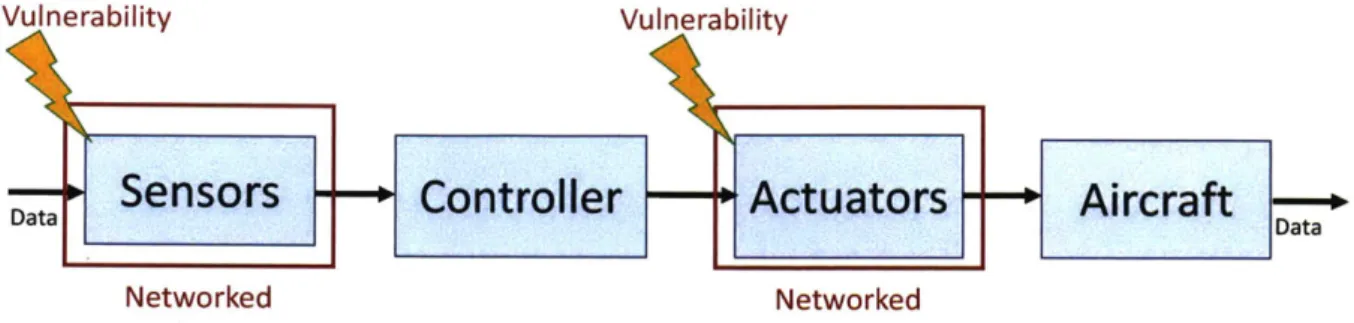
Over the past few decades, and with increasing intensity over the past few years, vast and complex dynamic control systems have relied on networked control schemes to seamlessly integrate parts and processes. These systems have come to be called Cyber-Physical Systems (CPS) and can be found in fields such as power, manufacturing, and transportation. As a result of this networked communication and control, components that were once separate or physically connected could no longer be treated as isolated from other parts of the system and the world, but rather in constant communication with them over potentially insecure channels. Thus, while networked communications enable flexibility in CPS, they introduce vulnerabilities in the form of potential entry points for corrupted data. As an example, corruption of vulnerable actuator and sensor channels of an an aircraft CPS, as shown in figure 1-1, has the potential to induce instabilities in the system as well as significant damage. While in the context of classical cyber-attacks, problems related to cyber security sought to contain the damage that could be done to information and cyber-processes, vulnerabilities in CPS now give us cause for concern about damaging and potentially unsafe outcomes in the physical world.

Concerns of cyber security arose out of the older field of information security (InfoSec) which developed significantly over the course of the 1970s. During this

Vulnerability Vulnerability

Sensors

Controller

Actuators

Aircraft

Networked Networked

Figure 1-1: Vulnerability of an Aircraft CPS

period, some of the first personal computers were introduced, as well as a variety of cheap and standardized software packages [2]. In 1975 Salzer and Schroeder classified three fundamental threats to information security: "unauthorized information release, unauthorized information modification, and unauthorized denial of use [191." In 1987, the Johnson Space Center labeled the corresponding security concerns as the CIA-triad, standing for Confidentiality, Integrity, and Availability [3]. These three pillars are commonly viewed as the backbone of a secure system. However, from the perspective of an adversary attempting to break security, these three pillars have corresponding threats that compromise the system according to vulnerabilities in each pillar. These threats or attacks are concisely summarized by Salzer and Schroeder's words and can be referred to as Disclosure, Deception, and Disruption attacks [1] or DDD attacks. [6] offers more in depth coverage of how CIA and DDD play out in CPS but it is not hard to see that the same defense and attack concepts that once applied to information security, now apply to cyber-physical systems.

Defender's Perspective Attacker's Perspective

Confidentiality

Disclosure attack - ex. eavesdrop

Integrity

Deception attack - corrupt signals

Availability

Disruption attack - block, delay

Figure 1-2: Fundamental Pillars of Securing and Compromising CPS

prevent, and mitigate attacks on CPS. In particular, much attention has been paid to fault and anomaly detection [13] as well as design for robust response

[5]

in the fields of estimation and control. While control theoretic methods of the past have treated anomaly detection and response in the cases where anomalies were viewed as exogenous disturbances, a control theoretic response for defense against CPS-attacks needs to account for a malicious actor who cannot be simply modeled as a random disturbance. Therefore, further research is warranted in designing systems that can detect and react to a malicious attacker. In this thesis, we develop a method by which a worst-case attack can be detected through a suitable analysis and design of a dynamic system.

In order to motivate the focus of the cyber-attack in this thesis, we return to two major attacks that have garnered significant attention. The first of these, Stuxnet, was a cyber-physical attack on an Iranian uranium enrichment plant resulting in damage

to approximately 1000 nuclear centrifuges

[7].

In targeting a commercially available

programmable logic controller (PLC) operating under a narrow set of conditions, the attackers were able to ensure that the attack reached its desired recipient with limited fallout [171. Stuxnet was designed to spy on industrial systems [15] and employed a cyber-attack tool, known as a rootkit, which enabled the malware to lie

dormant in the system and go undetected

1171.

This presents an opportunity for a

malicious attacker to perform reconnaissance, sitting quietly in a system undetected while, perhaps, observing critical and confidential system data. Upon observing sensor outputs of the system under stable conditions, the Stuxnet attack was able to replay those measurements, while injecting malicious actuation signals which did significant damage to a number of centrifuges [171.

The second major attack of interest is a cyberattack on the entire power grid of the country of Ukraine. In 2015 and 2016, a complex series of cyber attacks were launched on essential Ukrainian power distribution and transmission networks causing outages

as well as lasting damage

[8].

The 2015 attack was introduced to the network via

phishing emails containing the BlackEnergy malware. Once it infiltrated the system it enabled the attacker to steal critical system data and study the system environment,

enabling what would become a catastrophic attack [41 with effects on the Ukrainian power grid that have lasted to this day.

Motivated by the execution of the aforementioned attacks, this thesis envisions an attacker that starts their attacks by collecting useful and confidential data about the system. As mentioned above, the Ukraine attackers gained entry into the system through phishing emails, enabling access to confidential data. We propose a broader notion of an attacker "fishing" for confidential data, not restricted to emails as the

entry point of access. Both of the above examples show an attacker fishing for

confidential data which they can then use to construct critical system knowledge and as a result, develop a much more dangerous attack. For the duration of this thesis, we examine the security of CPS from both an attacker's perspective and a defender's perspective. The attacker's perspective is utilized to address how the attacker not only wants to infiltrate the system, but to gain critical and confidential system knowledge, such as the model parameters, in order to enable the design of an effective attack. As will be shown in subsequent sections, the stealthy and effective nature of this attack essentially causes the system to be driven to an unanticipated and possibly dangerous state with the defender unaware of the presence of the attacker. From the perspective of the defender, on the other hand, it is useful to design a system that not only keeps an attacker out, but alerts the defender to an attacker's presence and perhaps mitigates the effect of an attacker's actions. In what follows, we will refer to a successful, undetectable attack as stealthy and an unsuccessful attack as detectable. The specific cyber-attack model that we focus on in this thesis is that proposed in [11] which outlines a recipe for a stealthy attack on a flight control system. The authors of 111] assume that the attacker has access to a subset, if not all, of the actuator and sensor signals and can manipulate them, resulting in the deception attack shown in figure 1-3. In addition, the authors also assume that the attacker has full and accurate knowledge of the parameters of the linear dynamic system. It is then shown that the attack recipe ensures that the attacker can remain undetected and cause the estimation error to grow without bound. While the assumptions made in this paper are arguably unrealistic, one can view the attack recipe as a worst case.

Ua # Aircraft

E ac Attacker

a

₀

Controller

Figure 1-3: Deception Attack: Malicious injection of control and sensor signals.

Injected actuator attack, given by ac, and sensor attack, given by a0, cause the

control input that reaches the plant, Ua, and the sensor measurement that reach the

controller, Ya to be different from the uncorrupted u and y

In this thesis, we propose a defense mechanism to address this worst case, which is constructed so as to bait the attacker to reveal themselves.

Defense mechanisms that cause the attacker to be detected have been studied in a number of papers. The most notable of these are [17] and [201, and have been labeled as watermarking, since they correspond to authenticating signals of interest. Replay attacks of the kind conducted in the Stuxnet attack are considered in [17], and the

watermarking based defense mechanism consists of adding a random perturbation

to a standard feedback control input. In the presence of such a perturbation, any replayed signal will not be capable of producing a detection signal that corresponds to the correct distribution, and therefore enable attack detection. Care is taken to ensure that such a detection is enabled under minimal departure from the nominal feedback controller which is designed in an optimal manner. In [20], Satchidanandan and Kumar study the effects of this added perturbation signal on a more general set of sensor attacks and show that a set of uncompromised or "honest" actuators, each injecting their own added perturbation signal, can be used to check the honesty of the sensors which should report back measurements that contain some history of the perturbation signals' effects. More specifically, they analyze a number of systems including SISO and MIMO linear systems with gaussian noise, SISO ARX models, and SISO ARMAX models and show that the asymptotic behavior of a system with the perturbation signal constrains the damage a sensor-spoofing attacker can do while going undetected.

A second approach that has been used for attack detection is termed "moving target approach", an example of which is presented in

[241.

The attacker is assumed to have access to input-output channels, similar to [11], and therefore is capable of obtaining the true model parameters. The defense approach proposed then consists of augmenting the state vector with pseudo-states, the dynamics of which is created using a linear time-varying system and therefore difficult to carry out system identification on the associated model parameters. This in turn causes the underlying system to be a moving target and therefore difficult to stealthily attack. The specific use of such a time varying dynamics can be viewed as generating a watermark on the system which will enable authentication.

1.2

Contributions

In contrast to the watermarking approaches considered in the papers above, the method proposed in this thesis focuses on a parametric perturbation rather than an input perturbation or the addition of extraneous states. In contrast to replay attacks or the assumption that the attacker has knowledge of the system model, we assume the worst case recipe as in

[11]

which not only corresponds to a known system model but also full access to sensors and actuators which are then used to engage in the attack in a stealth mode. The parametric perturbation proposed will then be shown to bait the attacker into revealing themselves.

This thesis envisions an attacker that "fishes" for model parameter data in confidential documentation with the goal of using this model data to construct a stealthy attack. The objective of this attack is to generate large state estimation error while going undetected. To go undetected, the attacker's goal is to maintain a Kalman filter residual that looks identical to that of a healthy system. To ensure the attacker does not have a correct model, it is proposed that a defender anticipating this type of malicious intervention plants a falsified model in their documentation as bait for the fishing attacker. This falsified model contains the parametric perturbation discussed above. Upon employing the falsified model in their attack design, the baited attacker

Figure 1-4: Attacker Fishing for Model Data

1141

will reveal themselves by generating a Kalman filter residual that has a mean-shift from that of a healthy system.

While this first step of baiting enables the attack to be detected, this thesis proposes a second step in which observations of the residual combined with recursive least squares estimation offer an updated state estimate. Therefore, baiting will not only act to detect the presence of this class of stealthy attacks, but to enable more

accurate state estimation in the presence of these attacks.

The baiting approach proposed here can be viewed as similar to a cyber-security tool termed honeypot [211. This denotes an information system resource to guard against any probes, attacks, or compromises [221. For example, someone anticipating a cyber-attack, may use a secondary computer as a honeypot, acting as bait for an attacker to infiltrate. In this way, the honeypot can be used to detect attacks and even learn about the attacker's methods and capabilities [22]. A special type of honeypot, called a honeytoken, is a smaller, and often fabricated piece of data, rather than a larger system such as a computer [21]. In accessing and probing the honeytoken, which was not meant to be accessed or probed, the attacker might alert the defender to the intrusion [211. While the intended effect of the proposed baiting approach in this thesis is quite similar to these honeytokens, the application, as well as specific details associated with the methodology are quite distinct.

Motivated by a technique in which aircraft attempt to evade detection by enemy

defense method in which intentionally planted decoy exploits are placed in code. Military aircraft sometimes scatter aluminum strips, creating many sources of reflection for an enemy radar and ultimately making it hard for an enemy to detect an aircraft

among a host of decoys. These aluminum strips are called chaff. Therefore [91

refers to the bugs it uses as decoy exploits to stymie an attack as chaff bugs. Since attackers often look for bugs that can be used to exploit a system's vulnerabilities,

in introducing a significant number of intentionally placed benign chaff bugs,

191

proposes that an attacker will be forced to waste time and resources on trying to exploit many non-exploitable parts of the code. Like honeypots, this method is also conceptually similar to the baiting defense proposed in this thesis and reinforces how similar techniques are being explored in the field of cyber-security. We now extend our focus to the defense of CPS against stealthy attacks.

This thesis proceeds as follows: In chapter 2, we present a model of the dynamic system we will be studying as well as an attack model. Then, in section 2.3, we present a stealthy attack design. Chapter 3 develops a method to ensure that attacks are detectable and updated state estimates can be computed. The effects of the stealthy and detectable attacks on the lateral directional dynamics of an aircraft are simulated in chapter 4 and conclusions as well as suggested next steps are given in chapter 5.

Chapter 2

Models of the Dynamic System and

the Attack

2.1

Dynamic System Model

The starting point for our discussion is a dynamic system whose model is given by

x(k + 1) = Ax(k) + Bu(k) + Ejw(k) (2.1)

y(k) = Cx(k) + E₂v(k)

with the state x(k)

c

R"n, the input u(k) E Rtm, and the measured output y(k)

c

RP. In many cases n > p. Further w(k) ~ K(O,

Q),

and v(k) - K(O, R) are

uncorrelated process and output noises respectively, where - .A(pi, E) denotes a Gaussian distribution with mean it and covariance matrix E. A, B, C, E1, and E2 are all matrices of the appropriate dimensions and the system is assumed both controllable and observable. It is assumed that the state x is not measurable, and therefore needs to be estimated. Suppose that a standard Kalman filter is employed to estimate x

based on the measurements y using the following equations:

-(k + 1k) = AIc(k) + Bu(k)

x (k + 1) = (k + 1k) + Lr(k + 1) (2.2)

r(k + 1) =y(k + 1) - Cx-(k + 11k)

L is the steady state Kalman gain and is given by:

L = PaCT(CPaC + E2RE )-1 (2.3)

where Pa = E[(i(klk - 1) - x(k))(z(klk - 1) - x(k))T] is the steady state a priori

error covariance computed by solving the discrete time algebraic Riccati equation:

Pa = APaA + E1QEf - APaC(CPaCT + E2RE2T)-1 CPaAT (2.4)

The Kalman filter drives the steady state estimation error, e(k) A x(k) - -(k),

to a zero mean noise signal: e(k) ~ .A(O, P). P is the steady state estimation error

covariance given by:

P = (I - L)Pa (2.5)

Meanwhile, the difference between the measurement and the predicted measurement known as the residual, r(k), can be shown to be a zero-mean white noise signal of known variance [161: r(k) ~ A(0, E,) where E, is given by:

Er CPaCT + E₂RET (2.6)

While e(k) is the error in state estimate, r(k) is the error in the measurement prediction. It makes intuitive sense that these signals are both zero-mean noise terms in that an ideal filter of an observable system would converge to an unbiased estimate whose accuracy would be limited by the noises inherent to the system.

2.2

Attack Model

In [111, Kwon et. al assume that the system given by Equation (2.1) is attacked both at the input and at the output using attack vectors ac(k) and a0 (k) so that the

attacked system is of the form

Xa(k + 1) = Axa(k) + Bu(k) + Beac(k) + Elw(k) (2.7)

ya(k) = CXa(k) + Boao(k) + E2v(k)

ac(k)

E

R"c represents an injected attack on a subset of the actuators with Bc G Ra(B) and ao(k)

E

RPo represents an injected attack on a subset of sensors with B, C

Ra(C). The attacked system is assumed to have a state Xa and the corresponding

output is denoted as Ya. Further, it is assumed that the attacks are not injected until the system has reached steady state.

Suppose that a Kalman filter is used for the attacked system as

Xa(k + 1|k) = Axa(k) + Bu(k)

Xa(k + 1) = Xa(k + 1|k) + Lra(k + 1) (2.8)

ra(k + 1) =ya(k + 1) - Cia(k +

Ilk)

Ua * U Aircraft Y Dynamics Prediction

all, ao ra ra~N(0,I,.)?

z Attaker zAnomaly Detector

Controller

Figure 2-1: Deception Attack. An anomaly detector probes the Kalman filter residual to see if it exhibits the characteristics of a healthy system.

It follows that the corrupted residual ra(k) differs from r(k) due to the insertion of ac(k) and ao,(k). It also follows that under the unattacked case, the residual

how ra(k) differs from r(k) because of the attack inputs. As an example, we will consider the system under attack to be an aircraft. Figure 2-1 presents a schematic of the attack on an aircraft. The attacker injects a. into the control input to enforce that the input entering the control system, Ua, is different from that of the nominal control input, u, inducing unintended aircraft behavior. The attacker can also inject a, into the sensor outputs to feed the controller a corrupted output, ya, instead of the true output, y. The Kalman filter residual, which is the difference between the

measurement Ya and the expected measurement

y,

is then analyzed by an anomaly

detector to check if it has the expected characteristics of a healthy system.

Moving forward, we would like to analyze the potential effects of this attack from the perspective of the attacker. Let us assume that the attacker's objective is to generate non-zero state estimation error, ea, while going undetected. This stealthy attack will be achieved by designing the output attacks to mask the accumulated effect of the injected actuator attacks and therefore ensure that the resulting residual, ra, has a distribution identical to the residual of a healthy system, r [111. This results in potentially dangerous aircraft behavior that goes undetected by the defender. In the following subsection, we will investigate the effects of the actuator and sensor attacks and an attack design to achieve this stealthy attack.

2.3

Design of a Stealthy Attack

A common anomaly detection method for linear systems is to analyze the residual distribution. As previously discussed, in a healthy system, the defender expects a white residual distribution of zero-mean and known variance, E,. As is done in

[11],

algebraic manipulations of Equations (2.7) and (2.8) lead to the derivation of the residual of the attacked system as

where ea(k) Xa(k) - ,,(k) is the attacked system's state estimation error and has the following dynamic equation:

ea(k + 1) = GAea(k) + GBeac(k) + G E₁w(k) - LBoa0(k + 1) - LE2v(k +1) (2.10)

where GA I - LC.

Equation (2.10) can be taken k

+

1 steps back and be rewritten to reflect its complete history:

k-1 k-1

ea(k) = (GA)ke(0) + 1 (GA)zGBeac(k - 1 - i) + j (GA)tGEiw(k - 1 - i)

i=O i=O

k-1 k-i

-

S

(GA)2LBoao(k - i) - E(GA)LE2v(k - i) (2.11)

i=O i=O

whereas a healthy system error, e(k), does not have the attack terms:

k-i k-i

e(k) = (GA)ke(0) + 5(GA)'GEiw(k - 1 - i) - 5(GA)LE 2v(k - i) (2.12)

i=O i=O

Note that because the the attack does not begin until k = 0, at which point the

system has reached steady state, ea(0) = e(0) and therefore E[ea(0)] = E[e(0)] =

0. Therefore, upon further inspection of Equations (2.11) and (2.12), ea(k) can be written as the sum of the healthy system's state estimation error, e(k), and some attack terms:

k-1 k-1

ea(k) = e(k)+ (GA)'GBeac(k - I - i) - (GA)ZLBoao(k -i) (2.13)

written to reflect its complete history as well: k-i k-1 ra(k+l) =CA(GA)ke(O)+CAL(GA)GBcac(k-l-i)+CAZ(GA)GEiw(k-1-i) i=O i=O k-i k-i - CA L(GA)LBoao(k - i) - CA L(GA)'LE2v(k - i) i=O i=0

+ CBcac(k) + CEiw(k) + Boao(k + 1) + E2v(k + 1) (2.14)

and can similarly be written as a combination of the healthy system's residual and the effect of the attack terms:

k-i

ra(k + 1) = r(k + 1) + CA Z(GA)iGBeac(k - 1 - i)

k-i

-CA L(GA)LBoao(k -i)+CBcac(k)+ Boao(k +1) (2.15)

i=O

By designing the sensor attack to satisfy:

Boao(k + 1) = -C(AE[ea(k)] + Beac(k)) (2.16)

the attack terms in Equation (2.9) cancel and ra(k + 1) = r(k + 1) ~ J(O, E,) [11].

Equation (2.16) can be written more explicitly:

k+I

Boao(k + 1) = -C Ai-Bcac(k + 1 - i) (2.17)

Equation (2.16) is the pivotal equation proposed by Kwon et. al. which represents a recipe for a stealthy attack design and Equation (2.17) offers an algebraic view of this that will be useful for later manipulation. Note that just as the design given by Equation (2.16) canceled out the attack terms in Equation (2.9) for the residual dynamics, Equation (2.17) will cancel out the attack terms in the other representation of the residual given by Equation (2.15), again resulting in ra(k + 1) = r(k

+

1) ~

attacked system is identical to that of the healthy system, preventing the system defender from detecting the presence of an attack. Meanwhile, this choice of sensor attack, given by Equation (2.16), can be combined with the expectation of Equation (2.10) to give the mean state estimation error dynamics described by the following equation:

k+1

E[ea(k + 1)] = AE[ea(k)] + Bcac(k) = A'-1Beac(k + 1 - i) (2.18)

Taken together, Equations (2.18) and (2.16) represent the recipe for an attacker to choose ac(k) at each step so as to generate some desired and admissible error according to their attack objective and then recursively design the sensor attack,

a,(k + 1), which in turn cancels out the effect of the actuator attack on the residual,

enforcing that the attacked system has a residual distribution that is identical to that of the healthy system. In other words, an attacker chooses ac(k) according

to Equation (2.18) to generate state-estimation error and then designs a0(k + 1)

according to Equation (2.16) so as to erase any history of the actuator attack and prevent the defender from detecting the presence of this estimation error. This process can be viewed in figure 2-2.

at # Uy _{=yIlk+ y}

Aircraft _{Dynamics Prediction}

a a, -rI ra =r~N(0,p,.)

E jA

irc ra ftY

h +

E Attacker Anomaly Detector

Controller

U

_{Ya Yh}

Figure 2-2: Stealthy Attack Design. The attacker injects a, in order to induce

damaging system behavior and generate state estimation error, The resulting

measurement y is composed of a healthy signal, Yh, _{which would be the output of the}

system without ac, and a signal resulting from the input attack, '. The attack recipe then prescribes a sensor injection, a0, which cancels out the accumulated effect of the

actuator attack resulting in a residual that is identical to that of a healthy system. Note that Equation (2.16) can only be satisfied if the following condition holds

[11]:

Ra(C x ctrb(A, B,)) C Ra(B) (2.19)

where ctrb(A, B,) denotes the controllability matrix formed by the pair (A, Bc). Further, if the pair (A, B,) is controllable, the attacker has the potential to generate arbitrary state estimation errors 111].

Upon inspection of Equations (2.16) and (2.18), it becomes apparent that for an attacker to successfully implement the stealthy attack design, a number of things have to be available to the attacker. The first is that the attacker has the ability to modify the states using an attack input of the form Beac(k) at each k, so as to modify system behavior. Second, the attacker has sufficient access to the sensors, as given by Equation (2.19), to be able to modify the output using Boa0(k) at each k,

concealing the effect of the actuator attack. In addition, Equation (2.16) also assumes that the attacker has full knowledge of the matrices A and C which in turn amounts to knowing critical components of the system model. A major question of this thesis regards how robust this attack recipe is. That is, what happens when the attacker does not have perfect knowledge of the system model.

Chapter 3

Baiting For A Detectable Attack

3.1

Effect of Model Perturbation on Attack

In the previous section, a method was offered for an attacker with perfect model knowledge to induce potentially arbitrary state estimation error while going undetected, and quantified in the form of Equations (2.16) and (2.18). It is reasonable to raise the question as to how they attain this model knowledge, how accurate their knowledge is, and what the effect of an attack would be with a slightly inaccurate model. In this chapter, we investigate the effect of an attacker with an imperfect model. We will analyze how an imperfect model can lead to the attack becoming detectable. From the defender's perspective, it is then of interest to introduce such an imperfection into the attack-model. We will show that if the attacker is baited into such an inaccurate model, the defender can not only ensure that an attack is detectable, but can regain accurate state estimates.

We return to Equations (2.16) and (2.17). Suppose that there is an uncertainty A in A so that if we define Ab A A + A, the attacker uses Ab instead of A in Equations (2.16) (2.17). This perturbation modifies Equation (2.17) as

k+1

Using the fact that:

i-2

A'-1 = (A + A)'- A'-1 + E A'-2_{-jA(A + A)i (3.2)}

j=0

Equation (3.1) can be expanded as:

k+1 k+1 q-2

B_oa_o(k+l) = -CL Aq-1Beac(k+l-q)-CL

S

Aq-2-j (A+ j Beac(k+1-q)

q=1 q=2 j=O

(3.3) A comparison of Equations (2.17) and (3.3) shows that the effect of A introduces an additional second term not present in the attack model. More generally, we can say

at any instant k - i:

k-i k-i q-2

Boao(k-i) = -CEAq- Bcac(k-i-q)-C E Aq-2-ja A+AjBeac(k-i-q)

q=1 q=2 j=O

(3.4) Now, by inserting Equation (3.3) into the final term on the right hand side of Equation

(2.15), and inserting Equation (3.4) into the third term on the right hand side of Equation (2.15), we get an equation for the resulting faulty residual, rb, with some nominal attack terms that cancel each other out by design, and two terms generated by the modeling error introduced by the attacker:

k-2 k-i q-2

rb(k + 1) = r(k + 1) + CA 5(GA)LC

55

Aq-2-j A(A + A)3 Beac(k - i - q)

i=O q=2 j=0

k+1 q-2

- C Aq-2-jiA(A + A)3 _{Bcac_(k + 1 - q) (3.5)}

q=2 j=O

Equation (3.5) shows that the effect of an uncertainty A in the attack model causes the residue to change from r to rb instead of r to ra as in (2.15). That is, an attacker with a modeling error in A will induce a time varying shift in the mean of a healthy system's residual given by the last two terms in Equation (3.5). Because these two terms are a continuous function of A, there exists some C > 0 such that

for a sufficiently large A > E, E[rb(k + 1)] >

C

and the faulty attack is detected. Note that the deviation from the nominal residual induced by A is reminiscent of the effect of a watermarked input, similar to [17, 20]. Instead of an exogenous design of an additional perturbation signal in the control input on the part of the defender, any endogenous presence of a modeling error A on the part of the attacker may cause the attack to be revealed. In the next section, we discuss the effects of a defender enforcing such a A in the attack, thus intentionally "watermarking" the model.

3.2

A Defender's Perspective of the Baiting Approach

In order to ensure an attacker does not have a perfect model, the defender needs to anticipate how the attacker might acquire the model in the first place. It will be assumed that, as seen in a number of other attacks on CPS, the attacker fishes for model knowledge by infiltrating confidential systems, stealing enough data to construct the model, while remaining in a stealth mode. We propose that the defender, anticipating this type of infiltration, plants a deliberate perturbation A suggesting a slightly falsified model, Ab, thereby baiting an attacker fishing for data. This faulty model acts like a honeytoken, only to be used by an intruding attacker. The subscript b indicates a model that is used as bait for the attacker. This offers the defender the ability to choose A such that the use of Ab in the sensor attack design, given by Equation (3.1), is likely to result in a detectable attack.

Additionally, the combined effects of the attack and the faulty model yield the following equation for the state estimation error induced by a detectable attacker, eb:

k+1 k-2 k-i q-2

eb(k) = e(k)+YZ Aq 2 Beac(k+1-q)+I(GA)LC E 1 Aq-2-j A(A+A)jBeac(k-i-q)

q=2 i=O q=2 j=O

(3.6) The true state as a resulted of this baited attack is given by Xb and the defender's

naive estimate, before attempting to account for the effect of the attack, is given by

Xb. Note that ebb - Xb-x is composed of the healthy system's state estimation error

which is a zero mean noise series, a term yielding the effect of the stealthy attack, and a decoupled term induced by the fault in the model. Given that the defender can see rb, given by Equation (3.5), and more specifically, approximate the sum of the non-zero mean terms induced by A, it is of interest to see if it is possible to use that knowledge to reconstruct &b(k), an estimate of E[eb(k)] in Equation (3.6), and

therefore reconstruct a new more accurate state estimate, knew, using:

Xnew(k) = Xb(k) + eb(k) (3.7)

Equation (3.7) implies that not only does the use of A by the defender have the potential to make the attack detectable but it also provides an opportunity to get an updated and more accurate estimate - which includes the error &(k)

E[eb(k)]. In other words, A successfully baiting defender's choice of A makes the

attack detectable, but knowledge of that A makes it much easier to estimate Equation

(3.6) using Equation (3.5), improving the defender's state estimate.

Using Equations (3.5) and (3.6) to estimate eb(k) from observations of rb(k + 1) can be viewed as attempting to estimate the actuator attack, ac(k) for all prior k, enabling the calculation of the cumulative effect of the actuator attacks on the system dynamics. We will break up this estimation task into two cases. The first and more general case assumes that ac(k) is time varying, and therefore many, potentially distinct, values of ac(j) have to be estimated for all prior time j = 0... k. The

rather is a constant bias ac(k) = a,. For the general case where the attacker injects a time-varying actuator attack, ac(k), under appropriate conditions, weighted least squares can be used to solve a time-series representation of Equation (3.5) for ac(k)Vk. However, this method requires batch processing which will increase in complexity on each step and may therefore be intractable for real-time computations.

Let us proceed under the assumption that the attacker injects a constant bias as an actuator attack, that is, ac(k) = ac. Then, using Equation (3.5):

rb(k + 1) ~ A(M(k + 1)ac, E,) (3.8)

where

k-2 k-i q-2 k+1 q-2

M(k+1) = C(A Z(GA) LC

S S

Aq-2-j A (A+ A)i - E A- A (A +s Ai )Bc

i=O q=2 j=O q=2 j=O

(3.9) Therefore, ac can be estimated using recursive weighted least squares estimation under suitable rank conditions.

As a result of Equation (3.6):

eb(k) ~/(E[eb(k)], P) (3.10)

where

k+1 k-2 k-i q-2

E[eb(k)] = (5 Aq- 2 ₊

5

_(GA)TLC

5 5

_Aq 2_{-j A(A + AZj)Beac (3.11)}

q=2 i=O q=2 j=0

Therefore, using the least squares estimate a, at each step,

eb(k)

can be estimated

at each step and consequently, using Equation (3.7), -new(k), the updated and more accurate state estimate, can be computed at each step. The result of this analysis is that a defender that successfully baits an attacker fishing for model data can induce elements in the residual that not only make the attack detectable but re-enable accurate observations of the states, mitigating the effects of the attack.

3.3

Least Squares Implementation

In the previous section, we developed the baiting defense which enabled attack detection followed by updating the state estimates using recursive weighted least squares. In this section, we will give the steps that enable practical implementation of that recursive least squares update.

In the following, the time at which the attacker injects the actuator attack, ac, will be treated as k = 0. In practice, the defender will have to detect the presence of the attack based on some change in the residual, which will typically not be immediate. Therefore, the defender, seeking to estimate the effect of the attack on the states based on observations of the residual, will not know exactly when the attack was inserted. In other words, the defender does not know exactly when k = 0, only when the attack was detected. Attack detection will be discussed in further detail in Section 3.4.1.

In the following, it is assumed that the defender has an ideal detector such that the attack is detected immediately and they therefore know exactly what time corresponds to k = 0. In figure 4-2, we will see an example of how state estimation plays out in simulation when the time of detection is treated as k = 0 despite that not being the case. We will then look at cases where it is assumed that the defender has a better detector and therefore has a detection time that is closer to k = 0. This can also be thought of as the defender coming up with an estimate of how many steps prior to detection the attack must have occurred based on recordings of past residuals.

We will now develop the practical implementation of the recursive weighted least squares estimation method in which we use the observations of the baited residual to estimate a, and therefore enable improved state estimation. Upon inspection of Equations (3.8-3.9), we see that in that in order to execute each step of the recursive

least squares update, we need to to compute M(k

+

1) at each step. This computation

can be done efficiently by using a recursive formulation that computes M(k+ 1) based on a prior computation of M(k).

We can rewrite Equation (3.9) as follows:

M(k + 1) = C(AJ(k + 1) - Z(k + 1))Be

where

(3.12)

k-2 k-i q-2

J(k + 1) A Z(GA)LC Aq-2-jA(A + A)i

i=O q=2 j= O

k+1 q-2

Z(k + 1) A Aq-2-jA(A + A)i

q=2 j=O

If we define the following variables:

k-2 k-i-2

F(k +1) A ECGA) LC Ak-i-2-J A(A + A)3

i=0 j=0 k-2 V(k + 1) A Ak-2-jA(A + A) j=0 (3.13) (3.14) W(k + 1) A (A + A)k-2

then the following recursive formulation can be used to solve for J at each step:

W(k + 1) = W(k)(A + A)

V(k + 1) = AV(k) + W(k + 1) (3.15)

F(k +1) = GAF(k) + LCV(k +1) J(k + 1) = J(k) + F(k + 1)

with the following initial values:

J(1) = J(2) = 0

(3.16)

F(3) = LCA

Note that (3.15) along with (3.16) enable the iterative computation of J(k + 1)Vk.

Similarly, if we define the following:

k+1

H(k + 1) A (A + A)q-2

q=2 (3.17)

T(k + 1) A (A+ A)k-I

then the following recursive formulation can be used to solve for Z at each step:

T(k + 1) = T(k)(A + A)

H(k + 1) = H(k) + T(k + 1) (3.18)

Z(k +1) = AZ(k)+ AH(k +1)

with the following initial values:

Z(1) = 0

H(2) = In _(3.19)

T(2) = _Inxn

Z(2) = A

Note that Inx is the nxn identity matrix and as a reminder, G A I - LC. Equations (3.15,3.16,3.18,3.19) combined with Equation (3.12) enable a recursive calculation of matrix M(k + 1) based on the matrix at the previous step, M(k).

Now that we can construct M(k + 1) on each step, and we know the distribution of the baited residual is given by Equation (3.8), we have enough information to recursively update our estimate of a, on each step upon observation of the baited residual using the following recursive weighted least squares formulation [10]:

S(k + 1) = _{S(k) + MT(k + 1)E;-}1_{M(k + 1) (3.20)}

with the following initialization:

S(2) = MT(2)E;~'M(2)

ac(2) = S- 1_{(2)MT (2)E;-lrb(2)}

(3.21)

Now that we have a way of estimating and recursively updating ac, we want to use our estimate, a.c to estimate the state estimation error, eb using Equation 3.11. Equation 3.11 can be rewritten as:

E[eb(k)] = (N(k) + J(k + 1))Bcac (3.22)

where J(k + 1) is as defined in Equation (3.13) and N is given by:

k+1

N(k) I Aq-2

q=2

(3.23)

J(k + 1) can be recursively computed based on computations of J at past steps using

the iterations and initial conditions given by Equations (3.15-3.16). If we define

Y(k) A Ak-1 (3.24)

then N(k) can be recursively computed using the following formulation:

Y(k) = AY(k - 1)

(3.25)

N(k) = N(k - 1)+Y(k)

with the following initial conditions:

Y(1) = Inxn

N(1) = In

(3.26)

error db(k) by plugging our most up to date estimate of a, into the following:

&b(k) = (N(k) + J(k + 1))B.ac(k) (3.27)

Finally, we can get the most updated estimate of the state, , by adding this new

estimate of the state estimation error to the naive Kalman filter estimate of the state that we attained before this update, _b, using Equation (3.7).

3.4

Steps of the Baiting Defense Recipe

The aforementioned baiting defense can be thought of as broken down into two steps. The following elaborates on these steps and their execution to achieve the baiting defense.

3.4.1

Baiting: Step 1

The first step of the baiting defense consists of planting the false model given by

Ab - A

+

A and then detecting an attempted attack in the resulting residual shift given by Equations (3.5, 3.8).

Over the course of this thesis, we have focused on the residual as the signal that contains information about how close the system behavior is to nominal and developed conditions under which the residual will suggest departure from this nominal behavior. It is important that we discuss more specifically how we will determine a significant

departure has occurred in simulation and therefore detect an attack. In

[111,

Kwon

et. al choose to use a method called compound scalar testing which will be used in this thesis as well. This method computes a scalar function of the residual, referred to in [11] as the power of the residual, and given by:

r T (k)E r(k) (3.28)

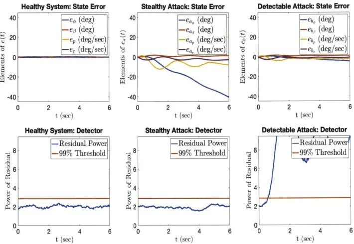
we expect in a healthy system, the power of the residual has an expected value of p, the dimension of r. A threshold h > p can then be chosen such that if rT(k)E;-lr(k) > h, the defender considers an attack to have occurred. In general, the choice of the detection threshold should depend on how we prioritize the detector's sensitivity to attacks against its sensitivity to false alarm. For the case of a baited attacker,

the resulting residual power, rs(k)E;'rb(k), should exhibit an increase compared

to that of a healthy system. For a large enough increase in the residual power and an appropriate choice of h, attacks should be detectable with low likelihood of false alarm.

3.4.2

Baiting: Step 2

Once the attack is detected, the residual of the Kalman filter can be observed to recursively estimate the injected actuator attack, ac, as explained in Section 3.3. Equations (3.12-3.21) give the necessary information to construct the matrix M at each step and use recursive weighted least squares so as to update the estimate of ac based on the observed residual at each step. For a sufficiently timely attack detection and a sufficient number of observations as well as a full rank M(k), the estimate of ac should converge to the true a,.

Similarly, Equations (3.22-3.27) give the necessary information to get an estimate of the induced shift in the state estimation error, eb(k) ~ E[eb(k)], by plugging the most updated estimate of a, into Equation (3.11). Before the update, the Kalman filter estimate is naive to the effect of the attack injections on the state estimation error. Equation (3.7) shows how at each step, this naive Kalman filter estimate, xb(k), can be added to the updated estimate of the state estimation error, eb(k) to yield the updated state estimate at that step, X ne(k). As the accuracy of a, improves with the number of observations of the residual, the accuracy of the state estimates should improve accordingly. Note that since recursive estimation is used, updated estimates are iteratively built on previous estimates and this technique can efficiently update state estimates in real-time.

3.5

Estimating Time of Attack Onset

In Section 3.3 we discussed how in practice, the defender does not know the exact time at which the attack was introduced, only the time at which the attack was detected. This, as we will see in Section 4.2.2, has the potential to result in an unideal step 2 state estimate. Ideal use of Equations (3.20-3.21) requires the defender to know when the attacked is introduced, so that the defender knows what step in the attack sequence, k, has been reached. We will see in Section 4.2.2 that as the attack detection time approaches the time of onset, the accuracy of state estimates resulting from step 2 of the baiting defense generally improves.

In this section we propose a method by which the defender can estimate the time of attack onset by looking at a recording of the residual signal for some prior period of time. In this method, the defender will record the residual until some time k = 1 where I occurs after the attack is detected. It is assumed that time I is sufficiently long after the attack onset, that there are sufficient observations of the residual to enable accurate estimation of a,. We will define acO(1) to be the estimate of ac resulting from baiting step 2 when the defender assumes the time of detection corresponds to

k = 0, the time the attack is introduced. As discussed in Section 3.3, the defender can

reasonably assume that their detection was not immediate and may therefore wish to estimate how many steps prior to detection the attack must have occurred. We therefore define &c (1) which is the result of baiting step 2, based on observations of the residual up to rb(l), and assumes the attack was introduced

j

steps before it was detected. That is, the defender has recordings of the residual signal for k up to k = 1, and at time 1 can get an estimate of ac using Equations (3.20-3.21) assuming that the time of attack onset is

j

steps before the time of detection. Unlike the method discussed in Sections 3.3-3.4, this method does not update the state estimates at each step but after a period of observation ending at time k = 1.

At time k = 1, the defender will estimate &cj(l) for a range of choices of j. This

corresponds to a range of guesses of how long before attack detection the attack onset took place. Then by replacing a, with &c3(l) in Equations (3.8-3.9), we can

define rbj(k + 1) to be the resulting estimate of mean residual, E[rb(k

+

1)], over the

defender's assumed attack time period. We can compare rb3 (k) to the recordings of

rb(k) over that assumed time period to get a root mean square error of our expected

residual when using &c

(l).

This will result in a root mean square error for every choice of j. The choice of

j

=

j*

that leads to the lowest root mean square error will then be chosen as an estimate of the number of steps before attack detection when the attack was introduced.

Now &^c*

(l)

is the defender's best estimate of a, resulting from estimating the time of attack onset prior to detection. Replacing a, with &c* (1) in Equations

(3.10-3.11) results in an estimate of the state estimation error for all k up to k = 1. Finally, this estimate of the state estimation error can be plugged into Equation (3.7) to yield an updated set of state estimates that takes into account the time of attack onset as distinct from the time of attack detection.

Chapter 4

Simulations

4.1

Preliminary Details

In this section we carry out simulation studies to validate the baiting approach proposed in Section 3. For this purpose, we use a nonlinear model of an F-16 outlined in [23] and further developed for simulation in [181. The model in Equation (2.1) will correspond to the linearized model of an F-16, and includes lateral-directional dynamics, assumed to be decoupled from the longitudinal dynamics as discussed in

[121.

A healthy system, that is one that is not under attack, will be simulated and compared to a system undergoing a successful stealthy attack as well as a system in which the attacker has been baited with a false model.

In Section 3.4.1, we discussed using the residual power as a metric for detecting attacks. A threshold can be defined such that if the residual power increases beyond that threshold, an attack is declared. In the following simulations, we will use a smoothed version of the power of the residual, resulting from a causal moving average filter. This smoothed signal is more sensitive to trends in the detection metric and in many cases makes it easier to detect the attack.

4.2

Simulation of a Non-Linear Dynamical System

The lateral-directional dynamics model of the F-16 operating near a straight and level steady cruise condition with an altitude of 15000 feet and a velocity of 500 feet per second can be approximated by the following linearized dynamic equation:

&cont =AconXcot + BcontUcont (4.1)

where the subscript cont denotes continuous dynamics. Acont and Bcont are assumed

to represent the plant with an inner loop control. The control input Ucont represents the aileron and rudder inputs of the aircraft:

Ucont= (4.2)

6ri

We will choose the following measurements:

ycont = 0 0 10 (4.3)

r 0 0 0 1 P

r

Though the dynamics are continuous, our technique is discrete and so sampling will be

required. Using a sampling time of T, = 0.01 seconds and adding zero-mean Guassian

process and measurement noises, Equation (4.1) is converted to a discrete time state space model of a form similar to the one given in Equation (2.1). In our application, there will be zero-mean Gaussian noise of ldeg/sec standard deviation on both sensor measurements and the process noise will be given as a Gaussian input disturbance with a standard deviation of 1% of the respective control surface maximum deflection. In order to deal with a particularly dangerous attack, we will look at the case where