RESEARCH OUTPUTS / RÉSULTATS DE RECHERCHE
Author(s) - Auteur(s) :
Publication date - Date de publication :
Permanent link - Permalien :
Rights / License - Licence de droit d’auteur :
Institutional Repository - Research Portal
Dépôt Institutionnel - Portail de la Recherche
researchportal.unamur.be
University of Namur
Recent progress in unconstrained nonlinear optimization without derivatives
Conn, A.R.; Scheinberg, K.; Toint, Ph.L.
Published in:Mathematical Programming Series B
Publication date: 1997
Document Version
Early version, also known as pre-print
Link to publication
Citation for pulished version (HARVARD):
Conn, AR, Scheinberg, K & Toint, PL 1997, 'Recent progress in unconstrained nonlinear optimization without derivatives', Mathematical Programming Series B, vol. 79, no. 3, pp. 397-414.
General rights
Copyright and moral rights for the publications made accessible in the public portal are retained by the authors and/or other copyright owners and it is a condition of accessing publications that users recognise and abide by the legal requirements associated with these rights. • Users may download and print one copy of any publication from the public portal for the purpose of private study or research. • You may not further distribute the material or use it for any profit-making activity or commercial gain
• You may freely distribute the URL identifying the publication in the public portal ?
Take down policy
If you believe that this document breaches copyright please contact us providing details, and we will remove access to the work immediately and investigate your claim.
Recent progress in unconstrained nonlinear optimization without derivatives by A.R. Conn1, K. Scheinberg2 and Ph.L. Toint3
Report 97/12 16 February 1997
1 IBM T.J. Watson Research Center, P.O.Box 218, Yorktown Heights, NY 10598, USA
Email: [email protected]
2 Industrial Engineering and Operations Resaerch Department, Columbia University, New York, NY 10027-6699, USA
Email: [email protected]
3 Department of Mathematics, Facult´es Universitaires ND de la Paix, 61, rue de Bruxelles, B-5000 Namur, Belgium, EU
Email: [email protected]
Current reports available by anonymous ftp from the directory “pub/reports” on thales.math.fundp.ac.be
WWW: http://www.fundp.ac.be/sciences/math/pht/publications.html
Recent progress in unconstrained nonlinear
optimization without derivatives
A. R. Conn K. Scheinberg Ph. L. Toint 16 February 1997
Abstract
We present an introduction to a new class of derivative free methods for unconstrained optimization. We start by discussing the motivation for such methods and why they are in high demand by practitioners. We then review the past developments in this field, before introducing the features that characterize the newer algorithms. In the context of a trust region framework, we focus on techniques that ensure a suitable “geometrical quality” of the considered models. We then outline the class of algorithms based on these techniques, as well as the associated global convergence theory. We finally conclude the paper with a discussion of open questions and perspectives.
1
Motivation
In this paper, we consider the problem of minimizing a nonlinear smooth objec-tive function of several variables when the derivaobjec-tives of the objecobjec-tive function are unavailable and when no constraints are specified on the problem’s variables. More formally, we consider the problem
min
x∈Rnf (x), (1.1)
where we assume that f is a smooth nonlinear function from Rn into R, and that∇f(x) (and, a fortiori, ∇2f (x)) cannot be computed for any x.
Our interest and motivation for examining possible algorithmic solutions to this problem is the high demand from practitioners for such tools. In the applications presented to the authors, computing the value f (x) given a vector x is typically very expensive, and the values of the derivatives of f at x are not available either because f (x) results from some physical, chemical or economet-rical measure, or, more commonly, because it is the result of a possibly very large and complex computer simulation, for which the source code is effectively unavailable. The occurrence of problems of this nature appears to be surpris-ingly frequent in the industrial world. In particular, the wider use of highly specialized, powerful but proprietary simulation packages makes the second of these situations increasingly common.
When users are faced with such problems, there are a few strategies that can be considered. The first, and maybe simplest, is to apply existing “direct
search” optimization methods, like the well-known and widely used simplex reflection algorithm of Nelder and Mead (1965) or its modern variants, or the Parallel Direct Search algorithm of Dennis and Torczon (1991) and Torczon (1991). This first approach has the merit of requiring little additional effort from the user, but may require substantial computing resources: the inherent smoothness of the objective function is not very well exploited, and, as a result, the number of function evaluations is sometimes very large, a major drawback when these evaluations are expensive.
The second and more sophisticated approach is to turn to automatic dif-ferentiation tools (see Griewank and Corliss (1991) or Griewank (1994), for instance). However, such tools are unfortunately not applicable in the two typ-ical cases mentioned above since they require f (x) to be the result of a callable program that cannot be treated as a black box.
A third possibility is to resort to finite difference approximation of the derivatives (gradients and possibly Hessian matrices). A good introduction to these techniques can be found in the book of Dennis and Schnabel (1983), for instance. In general, given the cost of evaluating the objective function, evaluating its Hessian by finite difference is much too expensive; one can use quasi-Newton Hessian approximation techniques instead. In conjunction with the use of finite differences for computing gradients, this type of method has proved to be useful and sometimes surprisingly efficient.
We will however focus here on a fourth possible approach, which is based on the idea of modeling the objective function directly, instead of modeling its derivatives. This idea seems particularly attractive in that one can replace an expensive function evaluation by a much cheaper surrogate model and, es-pecially for very complex problems, make considerable progress in obtaining improved solutions at moderate cost. The following interesting argument in favour of such techniques is for instance proposed by Powell (1974), where he considers the relatively simple problem of solving a single nonlinear equation. The idea is to compare, in this context, the secant method with the Newton-Raphson method. The first requires one function evaluation per iteration and has a convergence rate of approximately 1.618 per function value while the second requires one function and one derivative value per iteration and has quadratic convergence. Therefore, if an extra function value is used to estimate the derivative in the Newton-Raphson iteration, the mean rate of convergence per function value is only equal to √2. This simple example indicates that it may not be optimal to use function values to compute explicit derivative approximations.
We will group under the name derivative free optimization all methods which do not attempt to directly compute approximations to the unavailable deriva-tive information, but rather that calculate new and hopefully better iterates by considering a model of the objective function itself1. Our purpose in this paper is not to provide a detailed inverstigation of an algorithm, but rather to introduce some basic concepts for derivative free methods, and to outline a
1This class of methods can be coupled with some of the “direct search” approaches, see
whole class of algorithms in which these concepts are embodied.
The rest of the paper is organized as follows. After a short survey of the history of derivative free optimization techniques in Section 2, we investigate, in Section 3, the basic algorithmic features that characterize the newer methods. We then discuss at some length two possible approaches for the realization of some of the concepts needed in the proposed class of algorithms. Section 4 presents an approach based on the Lagrange fundamental polynomials, while Section 5 investigates the use of multivariate Newton interpolation techniques. We conclude the presentation by discussing open questions and perspectives in Section 6.
2
A brief review of derivative free optimization
meth-ods
It is difficult to firmly state where the idea of derivative free methods for mini-mization was first introduced, but it is clear that Powell was one of the first to systematically explore the potential of this approach. In Powell (1964), he de-scribed a method for solving the nonlinear unconstrained minimization problem based on the use of conjugate directions. The main idea of this proposal is that the minimum of a positive-definite quadratic form can be found by performing at most n successive line searches along mutually conjugate directions, where n is the number of variables. The same procedure may of course be applied to non-quadratic functions, adding a new composite direction at the end of each cycle of n line searches. Of course, finite termination is no longer expected in this case. This algorithm has enjoyed a lot of interest amongst both numer-ical analysts and practitioners. The properties of the method were analyzed by Brent (1973), Callier and Toint (1977), Toint and Callier (1977) and Toint (1978). The various computer programs based on this method have been widely used by a large number of practitioners2.
Aside from this line of thoughts, Winfield developped a different idea in his thesis at Harvard during the late 1960’s. His main idea, expressed in Winfield (1969) and Winfield (1973), is to use the available objective function values f (xi) for building a quadratic model by interpolation. This model is assumed to be valid in a neighbourhood of the current iterate, which described as a trust region (an hypersphere centered at xi), whose radius is iteratively adjusted. The model is then minimized within the trust region, hopefully yielding a point with a low function value. As the algorithm proceeds and more objective function values become available, the set of points defining the interpolation model are updated in such a way that its always contains the points closest to the current
2Powell made his method available in the Harwell Subroutine Library under the name
of VA04, but this original routine has been replaced by VA24, also written by Powell (see Harwell Subroutine Library, 1995). Brent (1973) gave an ALGOL W code named PRAXIS for a variant of the method. This latter code was subsequently translated to Fortran by R. Taylor, S. Pinski and J. Chandler. The Fortran version of PRAXIS is distributed in the public domain by J. Chandler, Computer Science Department, Oklahoma State University, Stillwater, Oklahoma 70078, USA ([email protected]). There is also an interface with the CUTEtesting environment of Bongartz et al. (1995).
iterate. This contribution is remarkable, not only because this idea (admittedly with some crucial modifications) forms the basis of the methods we wish to study here, but also because it appears to be a very early statement of a trust-region method, even before the seminal paper of Powell (1970). It is somewhat surprising that it went mostly unnoticed.
Both the method of Winfield and that of conjugate directions have proved to be reasonably reliable, but suffer from a main disadvantage: the need to maintain good linear independence of the successive steps. In the case of con-jugate directions, this is compounded with the relative difficulty of determining near-conjugate directions when the Hessian of the function is ill-conditioned. Recognizing these difficulties for this latter case, Powell (1974) suggested using orthogonal transformations of sets of conjugate directions. Pursuing this idea, Powell (1975) proposed to approximate the matrix of second derivatives itself, by modifying an initial estimate to ensure that it satisfies properties which would be satisfied if the objective function were quadratic. He also suggested the use of variational criteria, such as those used to derive quasi-Newton up-dates, in order that good information from an approximation can be inherited by its successors at subsequent iterations.
A few years later, Powell (1994a) proposed a method for constrained opti-mization, whose idea is close to that of Winfield. In his proposal, the objective function and constraints are approximated by linear multivariate interpolation3. Exploring the idea further, Powell (1994b) then described an algorithm for un-constrained optimization using a multivariate quadratic interpolation model of the objective function in a trust-region framework, an approach extremely sim-ilar to that of Winfield although seemingly independent. The crucial difference between Powell’s and Winfield’s proposals is that the set of interpolation points is updated in a way that preserves its geometrical properties, in the sense that the differences between points of this set are guaranteed to remain sufficiently linearly independent, therefore avoiding the difficulties associated with earlier proposals. A variant of this quadratic interpolation scheme was then discussed in Conn and Toint (1996), where encouraging numerical results were presented. Powell (1996) subsequently revisited this approach and showed similar com-putational results. The first convergence theorems for methods of this type were finally presented by Conn et al. (1997), together with a description of alternative techniques to enforce the desired geometrical properties of the set of interpolation points.
It is the purpose of the next section to investigate these crucial “geometry preserving” techniques, in the frameworks suggested by Powell and by Conn, Scheinberg and Toint.
3The associated Fortran code, named COBYLA, is distributed by Powell to interested
parties. An interface with the CUTE environment of Bongartz et al. (1995) is also provided for COBYLA.
3
A class of derivative free algorithms
The class of algorithms discussed in this paper belongs to the class of trust-region methods. Such algorithms are iterative and build, around the current iterate, a model of the true objective function which is cheaper to evaluate and easier to minimize than the objective function itself. This model is assumed to represent the objective function well in a so-called trust region, typically a ball centered at the current iterate, xk say, of the form
Bk={x ∈ Rn| kx − xkk ≤ ∆k} (3.1) The radius of this ball, ∆k, is called the trust region radius and indicates how far the model is thought to represent the objective function well. A new trial point is then computed, which minimizes or sufficiently reduces the model within the trust region and the true objective function is evaluated at this point. If the achieved objective function reduction is sufficient compared to the reduction predicted by the model, the trial point is accepted as the new iterate and the trust region possibly enlarged. On the other hand, if the achieved reduction is poor compared to the predicted one, the current iterate is typically unchanged4 and the trust region is reduced. This process is then repeated until convergence (hopefully) occurs.
The first main ingredient of a trust region algorithm is thus the choice of an adequate objective function model. We will here follow a well established tradition in choosing, at iteration k, a quadratic model of the form
mk(xk+ s) = f (xk) +hgk, si + 1
2hs, Hksi, (3.2) wherehx, yi denotes the usual Euclidean inner product between x and y, where gk is a vector of Rnand where Hkis a square symmetric matrix of dimension n. However, we will depart from many trust-region algorithms in that gk and Hk will not be determined by the (possibly approximate) first and second deriva-tives of f (·), but rather by imposing that the model (3.2) interpolates function values at past points, that is we will impose that
mk(y) = f (y) (3.3)
for each vector y in a set Y such that f (y) is known for all y∈ Y . Note that the cardinality of Y must be equal to
p = 1
2(n + 1)(n + 2) (3.4)
to ensure that the quadratic model is entirely determined by the equations (3.3). However, if n > 1, this last condition is not sufficient to guarantee the existence of an interpolant. For instance, six points on a line do not determine a two dimensional quadratic. Similarly, six interpolation points on a circle in the plane do not either, because any quadratic which is a multiple of the equation of
4This, of course, does not prevent the algorithm recording the best point found so far, and
the circle can be added to the interpolant without affecting (3.3). One therefore sees that some geometric conditions on Y must be added to the conditions (3.3) to ensure existence and uniqueness of the quadratic interpolant (see De Boor and Ron (1992) or Sauer and Yuan (1995), for more detail). In the case of our second example, we must have that the interpolation points do not lie on any quadratic surface in Rn or that the model chosen includes terms of degree higher than two. More formally, we need the condition referred to as poisedness, which relates directly to the interpolation points and the approximation space. If we choose a basis{φi(·)}pi=1 of the linear space of n-dimensional quadratics, we follow Sauer and Yuan (1995) and say that Y ={y1, . . . , yp} is poised when the “interpolation determinant”
δ(Y ) = det φ1(y1) · · · φ1(yp) .. . ... φp(y1) · · · φp(yp) (3.5)
is non-zero. Of course, the quality of the model (3.2) as an approximation of the objective function around xk will be dependent on the geometry of the con-sidered interpolation points and, from a practical point of view, it is important that we are able to measure this quality. It turns out that other measures than δ(.) are possible, and we will examine two possible choices in the next section. For now, we only need to assume that we know what we mean when we say that the geometry of Y is adequate (that is δ(Y ) is “sufficiently” different from zero), or when we say that we improve this geometry.
A second ingredient in trust-region algorithms is that one accepts a new point x+k produced by the algorithm as soon as f (x+k) is sufficiently smaller than f (xk), the current objective value. This is standard for trust-region methods, but the situation is more complex here because this means that we have to include x+k in the set of interpolation points Y . In general5, this means we need to remove another point y ∈ Y . Ideally, this point should be chosen to make the geometry of Y as adequate as possible. There are various ways to attempt to achieve this goal. We will again discuss some possibilities in the next section. It is important to note that, since xk+ sk is given irrespective of the geometry of the points already in Y , there is no guarantee that the quality of the geometry of Y will remain acceptable, or even that Y will remain poised, which opens the possibility that the quality of the geometry of Y might deteriorate as new iterates are accepted by the algorithm. This can happen, for instance, if successive iterates lie at the bottom of a steep valley whose shape may be described by a quadratic curve6. In such cases,|δ(Y )| may become very small, in which case we may question the relevance of our model.
As in all trust-region algorithms, we are also faced with the possibility that no further progress can be made from the current iterate xk. In algorithms using exact derivative information, Taylor’s theorem ensures that this problem must occur because the trust-region radius ∆kis too large, and thus guarantees that it disappears if ∆k is made sufficiently small. In our framework, on the
5Not necessarily so in the early stages of the algorithm.
6The bottom of the valley in Rosenbrock’s function is described by the equation x 2= x21.
other hand, we must also consider the possibility that the model’s quality is not adequate. This inadequacy could indeed result from the phenomenon described in the previous paragraph. If the algorithm is not able to progress, we thus have to check first if the geometry of Y is adequate, and, if it is not the case, we have to improve it. The desired improvement is achieved by introducing a new interpolation point y+ such that ky+− xkk ≤ ∆k in the set Y and using our measure of improvement to evaluate the replacement of some past point y− ∈ Y \ {xk} by y+, possibly comparing several choices for y−. This is the third main ingredient of our class of algorithms.
After this introduction to the main concepts, we may now outline this class as follows. We assume that the constants
0 < η0 ≤ η1 < 1, and 0 < γ0 ≤ γ1< 1≤ γ2, are given.
Outline of a derivative free trust-region algorithm Step 0: Initializations.
Let xsand f (xs) be given. Choose an initial interpolation set Y containing xs. Then determine x0 ∈ Y such that f(x0) = minyi∈Y f (yi). Choose an
initial trust region radius ∆0 > 0. Set k = 0. Step 1: Build the model.
Using the interpolation set Y , build a model mk(xk+ s), possibly restrict-ing Y to a poised subset containrestrict-ing xk, such that conditions (3.3) hold for the resulting Y .
Step 2: Minimize the model within the trust region. Compute the point x+k such that
mk(x+k) = min x∈Bk
mk(x). (3.6)
Compute f (x+k) and the ratio
ρkdef=
f (xk)− f(x+k) mk(xk)− mk(x+k)
. (3.7)
Step 3: Update the interpolation set.
• If ρk≥ η1, include x+k in Y , dropping one of the existing interpolation points.
• If ρk < η1 and Y is inadequate inBk, improve the geometry of Y in Bk.
Step 4: Update the trust-region radius. • If ρk ≥ η1, then set
∆k+1 ∈ [∆k, γ2∆k]. (3.8) • If ρk < η1 and Y was adequate in Bk when sk was computed, then
set
• Otherwise, set ∆k+1= ∆k. Step 5: Update the current iterate.
Determine ˆxk such that
f (ˆxk) = min yi∈Y yi6=xk f (yi). (3.10) Then, if ˆ ρkdef= f (xk)− f(ˆxk) mk(xk)− mk(xk+ sk) ≥ η0 , (3.11)
set xk+1 = ˆxk. Otherwise, set xk+1 = xk. Increment k by one and go to Step 1.
End of algorithm
Our outline is admittedly broad and simplistic. It is enough to consider the methods proposed by Powell (1994b), Conn and Toint (1996) or Powell (1996) to be convinced that practical algorithms involve a number of additional features that enhance efficiency. In particular, we haven’t mentioned a stopping test. A possible choice is to stop the calculation if either the trust-region radius falls below a certain threshold, or the model’s gradient becomes sufficiently small and the geometry of the interpolation set is adequate. However, our current description is sufficient to provide the framework of the discussion of the next section.
We also note that any further improvement in the model, compared to what the algorithm explicitly includes, is also possible. For instance, one might wish to include x+k in Y , even if ρk < η1, provided it does not deteriorate the quality of the model. Indeed, we have computed f (x+k) and any such evaluation should be exploited if at all possible. One could also decide to perform a geometry improvement step if ρk is very small, indicating a bad fit of the model to the objective function. Any further decrease in function values obtained within these steps is then taken into account by Step 5.
We finally mention that models other than full quadratics of the form (3.2) are also acceptable. This is necessary for the case where Y has to be restricted in Step 2 because it is not poised, in which case a model is built that does not include a contribution of functions chosen as basis of the space of quadratic polynomials. But other cases are also of interest. For instance, Conn and Toint (1996) suggest the use of models of degree exceeding two. Models that are less than fully quadratic or even less than fully linear are also beneficial when function evaluations are expensive since one is then able to use them as soon as they are available. This is typically the case at the first iterations of the algorithm, where simple models based on very few function values may be calculated and already exploited for decreasing the objective as soon as possible. We now return to the important question of providing a computable measure for the quality of the geometry of Y , which is necessary for substantiating the procedures of Step 3 for inclusion of x+k and geometry improvement. We examine two approaches.
4
An approach using the Lagrange fundamental
poly-nomials
The first approach is that of Powell (1994b) and Powell (1996). The idea is to measure the geometrical quality of the model by the value of the interpolation determinant δ(Y ) relative to its theoretical maximum. More precisely, we follow Powell (1994b) and say that the geometry of Y is adequate7 (with respect to a current iterate xk and a trust-region radius ∆) when all the points in Y are no further away from xkthan 2∆ and when the value of |δ(Y )| cannot be doubled by adjusting one of the points of Y to an alternative value within distance ∆ from xk.
We first consider improving the geometry of Y by introducing a new inter-polation point y+ such that ky+− xkk ≤ ∆ in Y (together with its associated function value f (y+)). This usually8 means that we have to drop an existing interpolation point y− from Y . We consider two cases. First, ifky−− xkk ≤ ∆, a suitable measure is |δ(Y )|, and we therefore wish to compute the factor by which |δ(Y )| is multiplied when y− is replaced by y+. Remarkably, this factor is independent of the basis {φi} and is equal to |L(y+, y−)|, where L(·, y−) is the Lagrange interpolation function whose value is one at y− and at all other points of Y is zero9. This very nice result was pointed out by Powell (1994b). Hence, ifky−− xkk ≤ ∆, it makes sense to replace y− by
y+= arg max ky−xkk≤∆
|L(y, y−)|. (4.1) On the other hand, ifky−−xkk > ∆, it is important to take this inequality into account when choosing a suitable replacement y+. One possible method is to compare y+not with y−directly, but rather with the best point on the segment joining xkto y− limited to the ball of radius ∆ around xk. This “scaled down” version of y− is the vector that maximizes|L(yc+ td−, yi)| for t ∈ [0, ∆], where d−= (y−− xk)/ky−− xkk. Hence, y+ may be chosen in this case as
y+= arg max ky−xkk≤∆ S(y, y−), (4.2) where S(y, y−) = |L(y, y−)| min[1, maxt∈[0,∆]|L(xk+ td−, y−)|] . (4.3)
The minimum in the denominator of (4.3) guarantees that the scaled down version of y−, namely arg maxt∈[0,∆]|L(xk+ td−, y−)|, is treated exactly as any other point within distance ∆ from xk (that is according to (4.1)). We may therefore define our improvement procedure as the replacement of y− by y+, where we have chosen y−to maximize S(y+, y−) for all choices of y− ∈ Y \{xk}, and where y+ is defined by (4.2), given y−.
Note also that the Lagrange interpolation function L(·, ·) is a quadratic determined by function value interpolation, and is therefore only well-defined,
7Powell uses the term “good”.
8It may not be the case at early stages of the algorithm. 9
together with S(·, ·), if Y is poised. Furthermore, problem 4.1 or (4.2) is thus of the same form as the trust-region subproblem (3.6).
The geometry of Y is then said adequate (with respect to xk and ∆) when ky − xkk ≤ ∆ for all y ∈ Y (4.4) and no point y+ can be found such that
ky+− xkk ≤ 2∆ and S(y+, y−) > 2 for at least one y−∈ Y \ {yc}. (4.5) If this is not the case, then a new point y+within distance ∆ of xk can be found if (4.4) is violated, or the point (4.2) can be used to replace the corresponding y− if (4.5) is violated. In this latter case the value of the replacement of y− by y+ is then given by S(y+, y−).
Note that verfying the adequacy of the geometry of Y not only involves checking (4.4), a relatively simple task, but also the solution of 2(p− 1) con-strained quadratic maximization problems. Indeed, we may write
max ky−xkk≤∆
S(y, y−) =
maxhmaxky−xkk≤∆L(y, y−),− minky−xkk≤∆L(y, y−)
i
min[1, maxt∈[0,∆]|L(xk+ td−, y−)|]
(4.6) and the two optimization problems of the numerator must be solved for each y− ∈ Y \ {xk}. This is not unreasonable since we have assumed that the cost of evaluating the objective function dominates all other costs, but neverthe-less constitutes a significant computational task when the number of problem variables grows.
To complete the description of the first approach, we only need to describe how we choose a point y− to drop from Y when we include x+k. Using the same idea as above, we see that a reasonable choice is to choose
y−= arg max y∈Y S(x
+
k, y−). (4.7)
One could also attempt to restrict the maximization, in this last definition, to the subset of Y consisting of points which are at a distance exceeding 2∆k, if such points exist. Or one might want to compromise between these two techniques by accepting a y− from the restricted set only if S(x,ky−) > 1 and resorting to (4.7) if no such point can be found.
Algorithms based on this first approach have been described in Powell (1994b), Conn and Toint (1996) and Powell (1996). Preliminary numerical results have been presented in the last two contributions, which indicate that remarkably efficient algorithms can be designed along this line.
5
An approach using Newton fundamental
polyno-mials
We now consider a second approach to measuring the quality of the geometry of Y , based on the properties of multivariate interpolation techniques. This
approach was introduced in Conn et al. (1997) with both a theoretical and a practical motivation. From the theoretical point of view, this approach allows global convergence to be proved for the associated version of our algorithmic outline. On the more practical side, this second approach sometimes signifi-cantly reduces the calculations performed by the algorithm on top of the objec-tive function evaluations. This is very desirable when the number of variables is not very small or when the cost of evaluating the objective function is not very high. At variance with the techniques of the previous section, we will empha-size here the use of Newton fundamental polynomials. It is important to realize that, if the interpolation techniques are different, the interpolating model is nevertheless unique whenever Y is poised. The reason for introducing a new interpolation technique is therefore not to modify the model for a given Y , but rather to derive from the new technique different procedures for improving the geometry of Y and for including x+k in the interpolation set.
In order to continue the discussion, we need to explore multivariate interpo-lation techniques a little further, which we do by considering the more general problem of finding interpolating polynomials of degree d. As above, we first choose a basis of the space of polynomials of degree d (for example the mono-mials) to initiate the process. In this framework, the point y in the interpolation set Y are organized into d + 1 blocks Y[ℓ], (ℓ = 0, . . . , d), the ℓ-th block contain-ing |Y[ℓ]| = ℓ+n−1
ℓ
!
points. To each point yi[ℓ] ∈ Y[ℓ] corresponds a single Newton fundamental polynomial of degree ℓ satisfying conditions
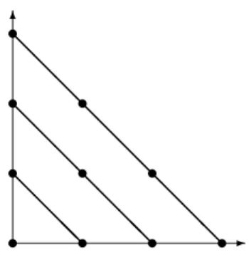
Ni[ℓ](yj[m]) = δijδℓm for all yj[m] ∈ Y[m] with m≤ ℓ. (5.1) For instance, if we consider cubic interpolation on a regular grid in the plane, we require ten interpolation points using four blocks
Y[0] ={(0, 0)}, Y[1] ={(1, 0), (0, 1)}, Y[2] ={(2, 0), (1, 1), (0, 2)} and Y[3]={(3, 0), (2, 1), (1, 2), (0, 3)}, as shown in Figure 1. 6 -@ @ @@ @ @ @ @ @ @ @ @ @ @ @ @ @ @ @ @ @ s s s s s s s s s s
Figure 1: Interpolation set and the four blocks (connected with thick lines) for cubic interpolation on a regular grid in the plane.
The interpolating polynomial m(x) is then given as m(x) = X
yi[ℓ]∈Y
λ[ℓ]i (Y, f )Ni[ℓ](x),
where the coefficients λ[ℓ]i (Y, f ) are generalized finite differences applied on f . We refer the readers to Sauer and Yuan (1995) for more details on these and multivariate interpolation in general.
We now return to the concept of poisedness and consider in more detail the procedure of constructing the basis of fundamental Newton polynomials as described in Sauer and Yuan (1995). Namely we consider the procedure below for any given Y .
Procedure CNP for constructing fundamental Newton polynomials
Initialize the Ni[ℓ] (i = 1, . . . ,|Y[ℓ]|, ℓ = 0, . . . , d) to the chosen polynomial basis (the monomials).
Set Ytemp =∅. For ℓ = 0, . . . , d,
for i = 1, . . . ,|Y[ℓ]|
choose some y[ℓ]i ∈ Y \ Ytemp such that|Ni[ℓ](y [ℓ] i )| 6= 0, if no such yi[ℓ] exists in Y \ Ytemp, reset Y = Ytemp and stop
(the basis of Newton polynomials is incomplete), Ytemp← Ytemp∪ {y[ℓ]i }
normalize the current polynomial by
Ni[ℓ](x)← Ni[ℓ](x)/|Ni[ℓ](yi[ℓ])|, (5.2) update all Newton polynomials in block ℓ and above by
Nj[ℓ](x)← Nj[ℓ](x)− Nj[ℓ](yi[ℓ])Ni[ℓ](x) (j 6= i, j = 1, . . . , |Y[ℓ]|), (5.3) Nj[k](x)← Nj[k](x)− N [k] j (y [ℓ] i )N [ℓ] i (x) (j = 1, . . . ,|Y[k]|, k = ℓ + 1, . . . , d). end
End (the basis of Newton polynomials is complete).
Clearly, poisedness relates to non-zero pivots in (5.2). Notice that after applying procedure CNP, Y is always poised since we only include the points that create non-zero pivots. This is true even if the procedure stops with an incomplete basis of Newton polynomials, which then results in an interpolating polynomial which is not of full degree d (meaning that it does not include contri-butions of all the monomials of degree d, see Step 2 of the algorithm). In practice we need sufficiently large pivots, which is equivalent to “well-poisedness”. Thus checking if |Ni[ℓ](y [ℓ] i )| 6= 0 is replaced by |N [ℓ] i (y [ℓ] i )| ≥ θ, for some θ > 0. We call θ the pivot threshold. In Conn et al. (1997), the authors have shown that if throughout the algorithm the interpolation problem can be made sufficiently
well-poised we are able to assure the existence of a bound on the distance between the interpolating polynomial and interpolated function at a point x (x 6∈ Y ). Otherwise we provide a mechanism that guarantees we can find a suitable interpolation for which the bound holds. This bound depends upon an important property proved by Sauer and Xu and uses the concept of a path between the zero-th block and x, which uses a sequence of points of Y of the form
π(x) = (y0[0], y1[1], . . . , y[d]d , y[d+1]d+1 = x) where
yi[i] ∈ Y[i] (i = 0, . . . , d).
A path therefore contains, besides x itself, exactly one interpolation point in each block. Let us denote by Π(x) ={π(x)}, the set of all possible paths from Y[0]to x. Using this notion, Sauer and Yuan (1995) derive in their Theorem 3.11 a bound on |f(x) − m(x)|, where m(x) is the polynomial interpolating the function f (x) at the points in Y . This bound was further simplified by Sauer (1996), giving that |f(x) − m(x)| ≤ n d+1kf(d)k ∞ (d + 1)! X π(x)∈Π(x) " d Y i=0 kyi+1[i+1]− y [i] i k∞|Ni[i](y [i+1] i+1 )| # , (5.4) for all x, where f(d) is the d-th derivative of f . Interestingly, the quantities Ni[i](yi+1[i+1]) are all computed in the course of the evaluation of the generalized finite differences λ[ℓ]i (Y, f ). We see that the error between m(x) and f (x) is smaller if we can make the values Ni[i](y[i+1]i+1 )kyi+1[i+1]− y
[i]
i k∞ small. If all the interpolation points and the point x are chosen in a given hypersphere of ra-dius δ, it is then possible to provide an upper bound on the maximal error. More precisely, the following theorem can be proved (see Conn et al. (1997), Theorem 2).
Theorem 1 Assume that an arbitrary xk ∈ Rn and a ∆k > 0 are given, together with the interpolation degree d. Then it is possible to construct an interpolation set Y yielding a complete basis of Newton polynomials such that all y∈ Y satisfy
y∈ Bk (5.5)
and also that
|Nj[ℓ](x)| ≤ κ0. (5.6) for all ℓ = 0, . . . , d, all j = 1, . . . ,|y[ℓ]| and all x ∈ Bk, and where the positive constant κ0 is independent of xk and ∆k.
We now return to the case of quadratic models of the form (3.2) and define what we mean by an adequate geometry of the interpolation set. In the spirit of Theorem 1, we assume that we are at iteration k of the algorithm, where xk is known (but arbitrary). We then say that Y is adequate inBk whenever the
cardinality of Y is at least n + 1 (which means the model is at least fully linear) and y∈ Bk for all y ∈ Y, (5.7) |Ni[ℓ](y [ℓ+1] j )| ≤ κ1 (i = 1, . . . ,|Y[ℓ]|, j = 1, . . . , |Y[ℓ+1]|, ℓ = 0, . . . , d−1), (5.8) and |Ni[d](x)| ≤ κ1 (i = 1, . . . ,|Y[d]|, x ∈ Bk), (5.9) where κ1 is any positive constant such that κ1 > κ0. (This choice of κ1 is merely intended to make (5.8) and (5.9) possible in view of Theorem 1.)
The inclusion of x+k in Y is then simply defined as follows: we may simply add x+k to Y if|Y | < p, and we need to remove a point y−of Y , if|Y | is already maximal (|Y | = p). Ideally, this point should be chosen to make the geometry of Y as good as possible. There are various ways to attempt to achieve this goal. For instance, one might choose to remove y− = yi[ℓ] such that |N
[ℓ] i (x)| is maximal, therefore trying to make the pivots as large as possible, but other techniques are possible.
The last procedure that we have to describe is the model’s geometry im-provement in Bk, which promotes making Y adequate in Bk. Again, many different techniques are possible. For instance, a reasonable strategy consists in first eliminating a point yi[ℓ] ∈ Y which is not in Bk (if such a point exists), and replacing it in Y by
y+= arg max x∈Bk|N
[ℓ]
i (x)|. (5.10)
If no such exchange is possible, one may then consider replacing interpolation points in Y \ {xk} by new ones, again using (5.10). The theory of Conn et al. (1997) then ensures that (5.8) and (5.9) hold after a finite number of such replacements. A computationally expensive version of the improvement proce-dure would compute y+ for every possible choice of y− = y[ℓ]i , and then select that for which |Ni[ℓ](y+)| is maximal, but substantially cheaper versions can be designed by choosing y− from the information which is already calculated when the interpolation model is computed. For instance, one may consider the vectors yi[ℓ] corresponding to polynomials for which|Nj[ℓ−1](y
[ℓ]
i )| is large for some j, or one may choose to replace fundamental polynomials corresponding to small pivots in Algorithm CNP. A closer look at the mechanism of this latter algorithm furthermore indicates that significant computational savings can be achieved if the polynomial to be replaced is selected in Y[d], or at least in the blocks of higher index, whenever possible.
The interested reader will find the global convergence theory associated with algorithms using this approach in Conn et al. (1997).
6
Discussion and perspectives
We have shown so far that one can design derivative free trust-region algorithms for unconstrained minimization in a variety of ways, but that it is important for
all these algorithms to take the geometry of the set of interpolation points Y into account. This is the main feature that distinguish modern methods from the proposal of Winfield (1969) and Winfield (1973). The crucial point is that this geometry should remain as adequate as possible, in the sense that the in-terpolation problem remains as far as possible from being ill-defined. We have examined two potential approaches that provide different manners to substan-tiate this requirement in practical computational methods. The first is based on the use of the Lagrange fundamental polynomials and is very elegant, if also potentially expensive in computing time. The second uses the Newton funda-mental polynomials and provides a framework for which global convergence can be proved for the resulting algorithm. It also suggests possible simplifications that reduce the computational complexity of the minimization method.
Significant work remains to be done for assessing the various possible algo-rithms discussed in this paper. In particular, it is desirable to explore to a much greater extent the computational tradeoffs between “best possible geometry” and acceptable amount of calculations as the relative cost of objective function evaluation and internal linear algebra varies. This work is currently ongoing and will be reported upon in the near future.
Besides this assessment, other questions of interest still need exploring. We have barely touched here the question of choosing initial models ate the early iterations of the algorithm, when the cardinality of Y doesn’t allow yet to define a full quadratic model. Many possible choices are possible, whose motivations may be as diverse as statistical design of experiments to analogies with the theory of “thin plate”spline functions. More questions related to the theoretical significance of pivot values in the context of Newton fundamental polynomials are also open and intersting.
An important direction for future work is the extension of the techniques discussed here to handle problems with a larger number of variables. One im-mediately thinks of exploiting any structure present in the problem as efficiently as possible. For instance, if the Hessian of the objective function has a known sparsity pattern, this fact can be exploited by suitably restricting the basis of monomials spanning the desired interpolation space: the monomial xixj may be removed from this basis if the (i, j)-th entry of the Hessian is known to be zero. Another possibility is to exploit partial separability (see Griewank and Toint (1982) or Conn et al. (1990)) in the objective function when possible. The idea would then be to build independent interpolation models for the ele-ments of the objective function, maybe coupled with a structured trust-region scheme (see Conn et al. (1996)).
Another direction of research, both useful and challenging, is to consider how the methods described here can be adapted to cases where some noise is present in the evaluation of the objective function. In this case, one expects that interpolation will be replaced by approximation in the model’s definition, and the conditions on geometry will have then to be combined with that of sufficient sampling.
Finally, the authors acknowledge that the potential of the methods outlined in this paper will only be fully realized when associated high quality software will become available to users. The development of such software is again the
subject of ongoing work.
To conclude our presentation, we wish to stress that derivative free methods for optimization remain a thriving and valuable area for research. It is indeed very encouraging that it presents such a remarkable combination of interesting theoretical concepts, useful algorithmic designs and high demand from potential users.
References
[Bongartz et al., 1995] I. Bongartz, A. R. Conn, N. I. M. Gould, and Ph. L. Toint. CUTE: Constrained and Unconstrained Testing Environment. Trans-actions of the ACM on Mathematical Software, 21(1):123–160, 1995.
[Brent, 1973] R. P. Brent. Some efficient algorithms for solving systems of nonlinear equations. SIAM Journal on Numerical Analysis, 10(2):327–344, 1973.
[Callier and Toint, 1977] F. M. Callier and Ph. L. Toint. Recent results on the accelerating property of an algorithm for function minimization without calculating derivatives. In A. Prekopa, editor, Survey of Mathematical Pro-gramming, pages 369–376. Publishing House of the Hungarian Academy of Sciences, 1977.
[Conn and Toint, 1996] A. R. Conn and Ph. L. Toint. An algorithm using quadratic interpolation for unconstrained derivative free optimization. In G. Di Pillo and F. Gianessi, editors, Nonlinear Optimization and Applica-tions, pages 27–47, New York, 1996. Plenum Publishing. Also available as Report 95/6, Dept of Mathematics, FUNDP, Namur, Belgium.
[Conn et al., 1990] A. R. Conn, N. I. M. Gould, and Ph. L. Toint. An introduc-tion to the structure of large scale nonlinear optimizaintroduc-tion problems and the LANCELOT project. In R. Glowinski and A. Lichnewsky, editors, Comput-ing Methods in Applied Sciences and EngineerComput-ing, pages 42–51, Philadelphia, USA, 1990. SIAM.
[Conn et al., 1996] A. R. Conn, N. I. M. Gould, A. Sartenaer, and Ph. L. Toint. Convergence properties of minimization algorithms for convex constraints using a structured trust region. SIAM Journal on Optimization, 6(4):1059– 1086, 1996.
[Conn et al., 1997] A. R. Conn, K. Scheinberg, and Ph. L. Toint. On the conver-gence of derivative-free methods for unconstrained optimization. In A. Iserles and M. Buhmann, editors, Approximation Theory and Optimization: Trib-utes to M. J. D. Powell, pages 83–108, Cambridge, England, 1997. Cambridge University Press.
[De Boor and Ron, 1992] C. De Boor and A. Ron. Computational aspects of polynomial interpolation in several variables. Mathematics of Computation, 58(198):705–727, 1992.
[Dennis and Schnabel, 1983] J. E. Dennis and R. B. Schnabel. Numerical Meth-ods for Unconstrained Optimization and Nonlinear Equations. Prentice-Hall, Englewood Cliffs, New Jersey, USA, 1983. Reprinted as Classics in Applied Mathematics 16, SIAM, Philadelphia, USA, 1996.
[Dennis and Torczon, 1991] J. E. Dennis and V. Torczon. Direct search meth-ods on parallel machines. SIAM Journal on Optimization, 1(4):448–474, 1991.
[Dixon, 1973] L. C. W. Dixon. ACSIM – an accelarated constrained simplex technique. Computer Aided Design, 5(1):22–32, 1973.
[Griewank and Corliss, 1991] A. Griewank and G. Corliss. Automatic Differ-entiation of Algorithms: Theory, Implementation and Application. SIAM, Philadelphia, USA, 1991.
[Griewank and Toint, 1982] A. Griewank and Ph. L. Toint. On the uncon-strained optimization of partially separable functions. In M. J. D. Powell, editor, Nonlinear Optimization 1981, pages 301–312, London, 1982. Aca-demic Press.
[Griewank, 1994] A. Griewank. Computational differentiation and optimiza-tion. In J. R. Birge and K. G. Murty, editors, Mathematical Programming: State of the Art 1994, pages 102–131, Ann Arbor, USA, 1994. The University of Michigan.
[Harwell Subroutine Library, 1995] Harwell Subroutine Library. A catalogue of subroutines (release 12). Advanced Computing Department, Harwell Labo-ratory, Harwell, Oxfordshire, England, 1995.
[Nelder and Mead, 1965] J. A. Nelder and R. Mead. A simplex method for function minimization. Computer Journal, 7:308–313, 1965.
[Powell, 1964] M. J. D. Powell. An efficient method for finding the minimum of a function of several variables without calculating derivatives. Computer Journal, 17:155–162, 1964.
[Powell, 1970] M. J. D. Powell. A new algorithm for unconstrained optimiza-tion. In J. B. Rosen, O. L. Mangasarian, and K. Ritter, editors, Nonlinear Programming, pages 31–65, London, 1970. Academic Press.
[Powell, 1974] M. J. D. Powell. Unconstrained minimization algorithms without computation of derivatives. Bollettino delle Unione Matematica Italiana, 9:60–69, 1974.
[Powell, 1975] M. J. D. Powell. A view of unconstrained minimization algo-rithms that do not require derivatives. Transactions of the ACM on Mathe-matical Software, 1(2):97–107, 1975.
[Powell, 1994a] M. J. D. Powell. A direct search optimization method that models the objective and constraint functions by linear interpolation. In
Advances in Optimization and Numerical Analysis, Proceedings of the Sixth Workshop on Optimization and Numerical Analysis, Oaxaca, Mexico, vol-ume 275, pages 51–67, Dordrecht, The Netherlands, 1994. Kluwer Academic Publishers.
[Powell, 1994b] M. J. D. Powell. A direct search optimization method that models the objective by quadratic interpolation. Presentation at the 5th Stockholm Optimization Days, Stockholm, 1994.
[Powell, 1996] M. J. D. Powell. Trust region methods that employ quadratic interpolation to the objective function. Presentation at the 5th SIAM Con-ference on Optimization, Victoria, 1996.
[Sauer and Yuan, 1995] Th. Sauer and X. Yuan. On multivariate Lagrange interpolation. Mathematics of Computation, 64:1147–1170, 1995.
[Sauer, 1996] Th. Sauer. Notes on polynomial interpolation. Private commu-nication, February 1996.
[Toint and Callier, 1977] Ph. L. Toint and F. M. Callier. On the accelerat-ing property of an algorithm for function minimization without calculataccelerat-ing derivatives. Journal of Optimization Theory and Applications, 23(4):531–547, 1977. Correction by F.M. Callier and Ph. L. Toint, same journal, vol. 26(3), pp. 465–467, 1978.
[Toint, 1978] Ph. L. Toint. Unconstrained optimization: the analysis of a con-jugate directions methods without derivatives and a new sparse quasi-Newton update. PhD thesis, Department of Mathematics, University of Namur, Na-mur, Belgium, 1978.
[Torczon, 1991] V. Torczon. On the convergence of the multidirectional search algorithm. SIAM Journal on Optimization, 1(1):123–145, 1991.
[Winfield, 1969] D. Winfield. Function and functional optimization by inter-polation in data tables. PhD thesis, Harvard University, Cambridge, USA, 1969.
[Winfield, 1973] D. Winfield. Function minimization by interpolation in a data table. Journal of the Institute of Mathematics and its Applications, 12:339– 347, 1973.