HAL Id: tel-01528568
https://tel.archives-ouvertes.fr/tel-01528568
Submitted on 29 May 2017
HAL is a multi-disciplinary open access
archive for the deposit and dissemination of
sci-entific research documents, whether they are
pub-lished or not. The documents may come from
teaching and research institutions in France or
abroad, or from public or private research centers.
L’archive ouverte pluridisciplinaire HAL, est
destinée au dépôt et à la diffusion de documents
scientifiques de niveau recherche, publiés ou non,
émanant des établissements d’enseignement et de
recherche français ou étrangers, des laboratoires
publics ou privés.
damage zones
Frans Aben
To cite this version:
Frans Aben.
Experimental simulation of the seismic cycle in fault damage zones.
Geophysics
[physics.geo-ph]. Université Grenoble Alpes, 2016. English. �NNT : 2016GREAU012�. �tel-01528568�
THÈSE
Pour obtenir le grade de
DOCTEUR DE L’UNIVERSITÉ GRENOBLE ALPES
Spécialité :
Sciences de la Terre, de l’Univers et de l’Environnement
Arrêté ministériel : 7thof August 2006Présentée par
Frans Aben
Thèse dirigée par
Mai-Linh Doan
et codirigée par
Francois Renard, Jean-Pierre Gratier
préparée au sein de
l’Institut des Sciences de la Terre
et de l’école doctorale
Terre Univers Environnement
Experimental Simulation of the
Seismic Cycle in Fault Damage
Zones
Thèse soutenue publiquement le
18
thof Novembre 2016,
devant le jury composé de :
Pascal Forquin, President
Enseignant-Chercheur, 3S-R, Université Grenoble Alpes, France, Président
Daniel R. Faulkner, Rapporteur
Professor, University of Liverpool, U.K., Rapporteur
Jean-Francois Molinari, Rapporteur
Professor, Ecole Polytechnique Fédérale de Lausanne, Switzerland, Rapporteur
Renaud Toussaint, Examinateur
Directeur de Recherche, Université de Strasbourg / CNRS, France, Examinateur
Tom M. Mitchell, Examinateur
Assistent Professor, University College London, U.K., Examinateur
Jean-Pierre Gratier, co-directeur
Emeritus Professor, ISTerre, Université Grenoble Alpes, France, Co-Directeur de thèse
Francois Renard, co-directeur
Professor, ISTerre, Université Grenoble Alpes, France & University of Oslo, Nor-way, Co-Directeur de thèse
R´
esum´
e
Les s´eismes le long de grandes failles crustales repr´esentent un danger ´enorme pour
de nombreuses populations. Le comportement m´ecanique de ces failles est influenc´e
par des zones endommag´ees qui entourent le coeur de faille. La fracturation dans ces
zones contrˆole chaque ´etape du cycle sismique. En effet, la zone endommag´ee contrˆole la
m´ecanique de la rupture sismique, se comporte comme un conduit pour les fluides, r´eagit
chimiquement sous l’effet de fluides r´eactifs, et facilite la d´eformation pendant les p´eriodes
post- et inter-sismiques. Cette zone est aussi un puits d’´energie pendant des grandes
ruptures sismique. Dans cette th`ese de doctorat, des exp´eriences de laboratoire ont ´et´e
r´ealis´ees pour mieux comprendre i) la fa¸con dont l’endommagement est g´en´er´e pendant
le chargement transitoire co-sismique d’une faille, ii) comment l’endommagement permet
de mieux contraindre le chargement co-sismique le long de grandes failles, et iii) comment
les fractures produites peuvent se cicatriser au fil du temps et contrˆoler l’´evolution de la
perm´eabilit´e et de la r´esistance m´ecanique de la faille.
L’introduction de la th`ese propose une revue critique de la litt´erature sur la g´en´eration
de dommages co-sismiques et en particulier sur la formation des roches pulv´eris´ees. Le
potentiel de ces roches comme marqueur des d´eformations co-sismiques et du m´ecanisme
de la rupture est discut´e. Bien que ces roches pulv´eris´ees soient prometteuses pour
ces aspects, plusieurs questions restent ouvertes. L’une de ces questions concerne les
conditions de chargement transitoire n´ecessaires pour atteindre la pulv´erisation. Le
taux de chargement critique pour atteindre la pulv´erisation peut ˆetre r´eduit par des
endommagements progressifs, au cours de ruptures sismiques successives. Des barres de
Hopkinson ont ´et´e utilis´ees pour effectuer des chargements successifs `a haute vitesse de
d´eformation d’une roche cristalline (monzonite riche en quartz). Les r´esultats montrent
que le seuil de taux de d´eformation pour atteindre la pulv´erisation est r´eduit d’au moins
50% lorsque des chargements successifs sont impos´es. Si la pulv´erisation n’est pas atteinte
lors de chaque chargement mais lors de chargements successifs, alors l’observation de
roches pulv´eris´ees sur le terrain indique que la pulv´erisation peut repr´esenter un ´etat
final d’endommagement plutˆot qu’un m´ecanisme d’endommagement en lui-mˆeme.
serv´ees dans des roches cristallines et peu dans des roches s´edimentaires plus poreuses,
mˆeme lorsque des roches cristallines et des roches s´edimentaires sont juxtapos´ees sur
une mˆeme faille active. Pour comprendre cette observation, des exp´eriences `a haute
vitesse de d´eformation ont ´et´e effectu´ees sur des gr`es poreux de Rothbach. Les r´esultats
montrent que la pulv´erisation des grains eux mˆemes, telle qu’observ´ee dans des roches
cristallines, ne se produit pas dans les gr`es pour la gamme de vitesses de d´eformation
explor´ee (60-150 s
-1. L’endommagement restant se produit principalement `a une ´echelle
sup´erieure `a celle grains, avec une d´eformation intra-granulaire se produisant seulement
dans certaines r´egions o`
u des bandes de compaction sont observ´ees. La comp´etition
entre l’endommagement inter- et intra-granulaire pendant le chargement dynamique est
expliqu´ee par les param`etres microstructuraux de la roche et en combinant deux
mod-`eles microm´ecaniques classiques: le mod`ele de contact Hertzien et le mod`ele de fissures
´emanant des pores. Les exp´eriences d´emontrent que les microstructures observ´ees dans
les gr`es peuvent se former `a la fois dans le r´egime de chargement quasi-statiques et aussi
dans le r´egime dynamique. Par cons´equent, il est recommand´e d’ˆetre prudent lors de
l’interpr´etation du m´ecanisme d’endommagement dans les roches s´edimentaires proches
de la surface aux abords d’une faille active. En conclusion, lors d’un chargement
tran-sitoire des r´eponses m´ecaniques diff´erentes de lithologies diff´erentes peuvent expliquer
l’asym´etrie des zones d’endommagement autour de certaines failles actives.
La derni`ere question abord´ee durant la th`ese est la cicatrisation post-sismique de
fractures co-sismiques. Des exp´eriences ont ´et´e r´ealis´ees pour cicatriser des fissures par
pr´ecipitation de calcite. Le but est l’´etude du couplage entre l’augmentation de r´esistance
m´ecanique de la roche fissur´ee et l’´evolution de la perm´eabilit´e du r´eseau de fractures.
Des r´eseaux de fractures ont ´et´e produits par chargement dynamique dans des
´echantil-lons de monzonite. Puis les ´echantil´echantil-lons ont ´et´e soumis `a des conditions de pression et
temp´eratures similaires `a celle de la croˆ
ute sup´erieure et `a une percolation d’un fluide
sursatur´e en calcite pendant plusieurs mois. Une augmentation importante de la vitesse
d’onde P a ´et´e observ´ee apr`es les exp´eriences avec une r´ecup´eration de 50% de la
diminu-tion initiale mesur´ee apr`es endommagement. En revanche, la perm´eabilit´e est rest´ee `a
peu pr`es constante pendant toute la dur´ee de l’exp´erience. Ce couplage non-existant
entre l’augmentation de r´esistance m´ecanique, mesur´ee par l’augmentation de la vitesse
des ondes P, et la perm´eabilit´e dans les premi`eres ´etapes de la cicatrisation est r´ev´el´e par
l’imagerie par tomographie aux rayons X de certains ´echantillons. Le scellement naissant
des fractures se produit dans les porosit´es situ´ees en aval de barri`eres d’´ecoulement, et
donc dans des r´egions qui ne touchent pas les principales voies d’´ecoulement du fluide.
Le d´ecouplage entre l’augmentation de r´esistance de la roche et l’´evolution de la
per-m´eabilit´e sugg`ere que les zones d’endommagement peu profondes dans les failles actives
peuvent rester des conduits actifs pour les fluides plusieurs ann´ees apr`es un s´eisme.
Abstract
Earthquakes along large crustal scale faults are a huge hazard threatening large
popula-tions. The behavior of such faults is influenced by the fault damage zone that surrounds
the fault core. Fracture damage in such fault damage zones influences each stage of the
seismic cycle. The damage zone influences rupture mechanics, behaves as a fluid conduit
to release pressurized fluids at depth or to give access to reactive fluids to alter the fault
core, and facilitates strain during post- and interseismic periods. Also, it acts as an
energy sink during large earthquake ruptures. Here, laboratory experiments were
per-formed to come to a better understanding of how this fracture damage is per-formed during
coseismic transient loading, what this fracture damage can tell us about the earthquake
rupture conditions along large faults, and how fracture damage is annihilated over time.
First, coseismic damage generation, and in particular the formation of pulverized fault
damage zone rock, is reviewed. The potential is discussed of these pulverized rock as
a coseismic marker that can be used to assess earthquake rupture mechanisms.
Al-though these rocks are promising in that aspect, several open questions remain. One
of these open questions is if the transient loading conditions needed for pulverization
can be reduced by progressively damaging during many seismic events. The successive
high strain rate loadings performed on quartz monzonites using a split Hopkinson
pres-sure bar reveal that indeed the pulverization strain rate threshold is reduced by at least
50%. Since dynamic fracturing is the damage mechanism during successive loadings,
rock pulverization is representative of an end-state of this damage mechanism rather
than of a damage mechanism by itself. Another open question is why pulverized rocks
are almost always observed in crystalline lithologies and not in more porous rock, even
when crystalline and porous rocks are juxtaposed by a fault. To study this observation,
high strain rate experiments were performed on porous Rothbach sandstone. The results
show that pervasive pulverization below the grain scale, such as observed in crystalline
rock, does not occur in the sandstone samples for the explored strain rate range
(60-150 s
-1). Damage is mainly occurs at a scale superior to that of the scale of the grains,
loading is explained with the geometric parameters of the rock in combination with two
classic micromechanical models: the Hertzian contact model and the pore-emanated
crack model. In conclusion, the observed microstructures can form in both quasi-static
and dynamic loading regimes. Therefore caution is advised when interpreting the
mech-anism responsible for near-fault damage in sedimentary rock near the surface. Moreover,
the results suggest that different responses of different lithologies to transient loading are
responsible for sub-surface damage zone asymmetry. Finally, post-seismic annihilation
of coseismic damage by calcite assisted fracture sealing has been studied in experiments,
so that the coupling between strengthening and permeability of the fracture network
could be studied. A sample-scale fracture network was introduced in quartz monzonite
samples, followed exposure to upper crustal conditions and percolation of a fluid
sat-urated with calcite for several months. A large recovery of up to 50% of the initial
P-wave velocity drop has been observed after the sealing experiment. In contrast, the
permeability remained more or less constant for the duration of the experiment. This
lack of coupling between strengthening and permeability in the first stages of sealing is
explained by X-ray computed micro tomography. Incipient sealing in the fracture spaces
occurs downstream of flow barriers, thus in regions that do not affect the main fluid flow
pathways. The decoupling of strength recovery and permeability suggests that shallow
fault damage zones can remain fluid conduits for years after a seismic event, leading to
significant transformations of the core and the damage zone of faults with time.
Contents
1
Coseismic damage generation and pulverization in fault zones: insights
from dynamic Split-Hopkinson Pressure Bar experiments
13
1.1
Introduction . . . .
16
1.2
Field observations of pulverized rock related to coseismic damage . . . .
18
1.2.1
Observations, definition and microstructures of pulverized rock . .
18
1.2.2
Pulverized rock at the fault system scale . . . .
22
1.3
Coseismic off-fault damage by analogous laboratory experiments . . . . .
26
1.3.1
General overview of the strain rate sensitivity of geomaterials . .
26
1.3.2
Coseismic damage by compressional loading experiments . . . . .
28
1.3.3
Dynamic tensile loading SHPB experiments . . . .
41
1.4
Dynamic brittle damage models . . . .
43
1.4.1
Dynamic versus quasi-static damage: strain rate effects on a
net-work of microfractures . . . .
43
1.4.2
Models constraining the decrease in grain size with increasing strain
rate . . . .
44
1.4.3
Models constraining the increase in strength with increasing strain
rate . . . .
48
1.5
Discussion . . . .
53
1.5.1
Is long-distance pulverization by sub-Rayleigh wave speed ruptures
possible? . . . .
53
1.5.2
Alternative conditions for coseismic pulverization . . . .
57
1.5.3
Damage anisotropy and loading conditions . . . .
60
1.5.4
Other implications for fault zones . . . .
61
1.6
Perspectives and conclusion . . . .
63
2
Dynamic fracturing by successive coseismic loadings leads to
2.1
Dynamic fracturing by successive coseismic loadings leads to pulverization
in active fault zones . . . .
75
3
High strain-rate deformation of porous sandstone and the asymmetry
of earthquake damage in shallow fault zones
99
3.1
Introduction . . . 101
3.2
Material and methods . . . 103
3.2.1
Sandstone samples . . . 103
3.2.2
Experimental setup . . . 104
3.3
Results . . . 106
3.3.1
Macroscopic damage . . . 106
3.3.2
Mechanical data . . . 106
3.3.3
Microstructures . . . 110
3.4
Discussion . . . 114
3.4.1
Micromechanical damage models . . . 114
3.4.2
Effect of pore fluids on dynamic damage . . . 119
3.4.3
Anisotropy effect on damage mechanism . . . 119
3.4.4
Dissipated energy and deformation mechanism . . . 120
3.4.5
Dynamic damage across bimaterial fault zones . . . 120
3.5
Conclusion . . . 122
4
Experimental post-seismic recovery of fractured rocks assisted by
cal-cite sealing
129
4.1
Introduction . . . 131
4.2
Experimental method . . . 133
4.2.1
Description of the triaxial pressure cells . . . 133
4.2.2
Description of the fluid percolation system . . . 135
4.2.3
Sample preparation . . . 138
4.2.4
Setup of healing experiments . . . 139
4.3
Results . . . 140
4.3.1
Initial damage . . . 140
4.3.2
Mechanical results . . . 141
4.3.3
Fluid flow results . . . 145
4.3.4
Microstructures . . . 149
4.3.5
Fluid chemistry . . . 155
4.4
Discussion . . . 158
CONTENTS
4.4.2
Strengthening . . . 158
4.4.3
Coupling between permeability and strengthening . . . 160
4.5
Conclusion: Implications for post-seismic recovery . . . 162
Conclusions and further research
169
4.6
Suggestions for further research . . . 170
A Supporting information for Dynamic fracturing by successive
coseis-mic loadings leads to pulverization in active fault zones
175
A.1 Supporting Information A: Split Hopkinson Pressure Bar: method,
as-sumptions and pitfalls . . . 175
A.2 Supporting Information B: Porosity computation from X-ray CT data . . 182
A.2.1 2D analysis . . . 182
A.2.2 3D analysis . . . 182
A.3 Supporting Information C: The onset of dynamic fracturing
. . . 182
A.3.1 Theoretical considerations . . . 183
A.3.2 High speed camera . . . 185
B Supporting Information for High strain-rate deformation of porous
sandstone and the asymmetry of earthquake damage in shallow fault
zones
191
B.1 Pore space from image analysis . . . 191
B.2 An in-depth analysis of the pore-emanated crack model and the chosen
assumptions . . . 192
Chapter 1
Coseismic damage generation and
pulverization in fault zones: insights
from dynamic Split-Hopkinson
Pressure Bar experiments
This first chapter is an extensive review on the field observations on pulverized rock, the
experimental laboratory methods used to study such rock and the current
experimen-tal knowledge. Further, various damage models capable of predicting a pulverization
threshold are discussed. Finally, the field and experimental observations are integrated
using rupture models. Also, open questions are highlighted regarding pulverized rocks
as a coseismic marker. This paper has been accepted for the AGU book ”Evolution of
Fault Zone Properties and Dynamic Processes during Seismic Rupture”, edited by M.Y.
Thomas, H.S. Bhat and T.M. Mitchell.
abstract
Coseismic damage in fault zones contributes to the short- and long-term behavior of a
fault and provides a valuable indication of the parameters that control seismic ruptures.
This review focuses on the most extreme type of off-fault coseismic damage: pulverized
rock. Such pervasively fractured rock, that does not show any evidence of shear strain, is
observed mainly along large strike-slip faults. Field observations on pulverized rock are
briefly examined and would suggest that dynamic (high strain rate) deformation is
respon-sible for its generation. Therefore, these potential paleo-seismic markers could give an
indication of the constraints on rupture propagation conditions. Such constraints can be
determined from dynamic loading experiments, typically performed on a Split-Hopkinson
Pressure Bar apparatus. The principle of this apparatus is summarized and
experimen-tal studies on dynamic loading and pulverization are reviewed. For compressive dynamic
loading, these studies reveal a strain rate threshold above which pulverization occurs. The
nature of the pulverization threshold is discussed by means of several fracture mechanics
models. The experimental pulverization conditions are correlated with field observations
by analyzing and discussing several earthquake rupture models. An indisputable rupture
mechanism could not be established owing to a gap in experimental knowledge, especially
regarding tensile dynamic loading.
List of symbols
A Surface area
AB, AS (bar, sample)
cd P wave velocity (velocity of dilatational stress wave) cs S wave velocity (velocity of shear stress wave) D Fractal dimension (section 1)
D Damage parameter (section 4)
D Rayleigh function (section 5)
d Displacement of cohesive elements (section 4)
E Young’s modulus
ǫ Strain
˙ǫ Strain rate
˙ǫ0 Characteristic strain rate (=threshold in strain rate for pulverization)
F Force
FI, FR, FT (incident, reflected, transmitted)
G Energy release rate
GC Critical energy release rate
K Stress intensity factor at a crack tip
KII Stress intensity factor at a mode II crack tip ˙
K Stress intensity factor rate (= time derivative of K) KC Fracture toughness (= critical stress intensity factor) Kd
C Dynamic fracture toughness (= critical stress intensity factor)
L Length of the sample
l0 Initial density of flaws in the solid m Shape parameter of Weibull function
n Dimension of the model
N Number of fragments
ν Poisson’s ratio
θ Angle to the rupture plane (used in polar coordinates) r Distance from rupture tip (used in polar coordinates) R Grain size characteristic radius
ρ Mass density
s Size of individual fragments after fragmentation (=radius for spherical fragments) s0 Characteristic fragment size
σ Stress
σC Critical stress for activation of an individual flaw Σ Angular stress variation at the crack tip
τ Particle (in the sense on continuum mechanics)
v Particle velocity (section 3 and 4) / Rupture velocity (section 5)
UK Kinetic energy
V Volume of the sample
1.1
Introduction
Damage to rock formations surrounding faults can have a major influence on the
me-chanical behavior of the faults, whether they are seismogenic or aseismically creeping
faults. Fracturing may increase, at least temporarily, the permeability of the damaged
rock, leading to episodic fluid flow that modifies its rheological properties [Sibson, 1996;
Miller, 2013]. Fracturing may contribute to the development of anisotropy around the
fault zone [Crampin and Booth, 1985; Zhao et al., 2011] and may also activate
chemi-cal reactions facilitating stress-driven mass transfer creep [Gratier et al., 2013a, 2014].
Subsequent sealing of the fractures may strengthen the rock, contributing to mechanical
segregation in a fault zone and possibly leading to localized earthquakes [Li et al., 2003;
Zhao et al., 2011; Gratier et al., 2013b]. Such a heterogeneity could in turn be a tuning
parameter in fault slip and earthquake dynamics [B¨urgmann et al., 1994; Z¨oller et al.,
2005].
Conversely, the behavior of the fault itself influences the amount and type of damage
occurring in the damage zone [Faulkner et al., 2011]. This damage may be caused by a
variety of quasi-static and dynamic deformation processes [Mitchell and Faulkner, 2009].
The mutual interaction between fault and damage zone is not yet fully understood,
es-pecially the long-term effects, including gradual chemical changes of the fault core gouge
that might change the behavior of the fault zone from seismic to aseismic permanent
creep [Richard et al., 2014]. Consequently, damage development processes in faults are
a crucial factor in understanding the mechanics of faults.
Within the damage zone, coseismically damaged rock formations provide a means
of constraining fault and earthquake mechanics given that they were formed by seismic
events. Coseismically damaged rocks differ from other damage zone rocks inasmuch that
they are dynamically loaded in tension or compression by stress waves surrounding a
propagating rupture tip for a short duration. Due to dynamic loading, the kinetics of
fracture propagation controls the damage process [Grady, 1998] and not just the local
state of stress as is the case for quasi-static crack growth.
The most extreme coseismic end-member is thought to be pulverized rock and
there-fore this rock has the highest potential both as a seismic marker and as a process that
drastically modifies the mechanical properties of the fault zone. Pulverized rocks are in
situ exploded rocks that have been subjected to pervasive fracturing up to the
microme-ter scale, without any accumulation of shear strain. The fracture damage is mechanical
in nature and this type of rock is almost exclusively present in the top few kilometers
along major strike-slip faults. Such rock could potentially be indicative of one or several
1.1 Introduction
paleoseismic events. Moreover, these rocks might give constraints on the magnitude,
loading conditions and rupture direction. For the time being, such constraints remain
open questions.
Since being acknowledged as a source of information for earthquake events by Brune
[2001] and Dor et al. [2006a], research on these rocks is still in a preliminary phase. A
strict definition including more than the qualitative description given above has not yet
been established for this type of rock. Furthermore, the factors setting these rocks apart
from their lesser coseismically damaged peers in terms of damage process have yet to be
defined.
These questions can partly be answered by mapping the processes and conditions
in which pulverized rocks can be formed. This also includes studying non-pulverized
coseismically damaged rocks to constrain the entire range of fracture damage products
that might be expected during a seismic event. To this end, laboratory experiments are
crucial whereby samples are exposed to stress wave loading, similar to the high frequency
waves emitted during an earthquake. In contrast to many other physical and mechanical
experiments on rocks, a time transformation from laboratory loading rates to natural
loading rates is not necessary; rather the challenge is to simulate the fast loading rates
of a seismic rupture.
This review-style chapter starts with a summary of field observations on pulverized
rock, including an outline of the issues regarding the definition of a pulverized rock. The
current state-of-the-art of high loading rate experiments will then be presented, first
in general form and secondly for pulverization in particular. Since these experimental
studies are performed mostly on the Split-Hopkinson Pressure Bar apparatus, a short
overview of this technique is given. More details are then given of current dynamic
fracture models and theories in the high strain rate regime to explain the transition
to pulverized rocks. Finally, current experimental knowledge and field observations are
linked to earthquake rupture mechanical models and their implications for fault zones
containing pulverized rocks are discussed.
1.2
Field observations of pulverized rock related to
coseismic damage
1.2.1
Observations, definition and microstructures of
pulver-ized rock
The first observations of pulverized rocks were at or near the surface along the San
Andreas fault between San Bernardino and Tejon pass on granites and gneisses [Brune,
2001; Dor et al., 2006a]. Prior to this, these rocks might have been overlooked or labeled
as gouges and cataclasites after the classic definition [Sibson, 1977; Wilson et al., 2005].
However, the features setting them apart from these classic fault zone rocks are well
summarized in the field definition given by [Dor et al., 2006a]: A rock is classified as
pulverized when the original textures are preserved (Figure 1.1a), very little or no
shear is visible and all the crystals in a sample yield a powdery rock-flour texture when
pressed in the hand. This damage is widespread on the outcrop scale. At the field-scale,
these rocks can be easily recognized due to their badland type morphology [Dor et al.,
2006a,b, 2008; Mitchell et al., 2011] (Figure 1.1b) and faster erosion rate compared to
the surrounding rocks.
On a smaller scale, pulverized igneous crystalline rocks (granite, granodiorite, gneiss)
are characterized by a large number of fractures seemingly oriented randomly in 3D and
without any clear hierarchical organization (Figure 1.1c-d). The fracture density is very
high and, in general, the fractures penetrate all mineral phases, although some harder
minerals may contain fewer fractures in places where the rock is less pulverized. Fracture
patterns can be either random or follow cleavage planes, and micas can be kinked or
contain fewer fractures than other mineral phases (Figure 1.1e). The dilatational mode
I fractures show very little offset and the fragments bounded by the fractures show little
to no rotation, as evidenced by cross-polarized images in which original grains can be
clearly identified from the myriad of fragments (Figure 1.1f-g). Since weathering might
alter granitic rocks towards a more fragile lithology, several authors have conducted
mineralogical studies that have ruled out this mechanism [Rockwell et al., 2009; Mitchell
et al., 2011; Wechsler et al., 2011] and they have proposed a mechanical origin instead.
This, together with the microstructures, indicates a mechanical source for pulverization.
In some studies, geometric analyses have been conducted to characterize crystalline
pulverized rocks in greater detail. Particle size distributions (PSD) were obtained on San
Andreas pulverized rocks by Wilson et al. [2005], Rockwell et al. [2009] and Wechsler
et al. [2011] using a specially calibrated laser particle size analyzer. The results indicated
1.2 Field observations of pulverized rock related to coseismic damage
(a)
(b)
(c)
0.2 mm(e)
1 mm(f )
X-polarized II-polarized 0.5 mm(d)
0.5 mmFigure 1.1: (a) Image of a pulverized granite showing a clear pristine crystalline texture. (b)
Typical badland erosion geomorphology related to pulverized rocks. (c)-(e) Photomicrographs
of pulverized granitic rocks. (c) is taken with parallel polarizers, (d) and (e) with crossed
polarizers. (e) contains a slightly buckled biotite grain. (f ) Photomicrographs with parallel
(left) and crossed (right) polarizers show that hardly any rotation or movement of fragments
has occurred. (a), (b) from Mitchell et al. [2011], (c) from Rempe et al. [2013], (d) from
Wechsler et al. [2011], (e) from Muto et al. [2015] and (f ) from Rockwell et al. [2009].
non-fractal PSD behavior towards larger grain sizes (>500 µm). For smaller grain sizes
(0.5-500 µm) a D-value fractal exponent in the range 2.5-3.1 provided the best power
law fit. Moreover, Wilson et al. [2005] constrained surface areas of up to 80 m
2/g,
although it is not clear whether this was actual gouge or pulverized rock. Muto et al.
[2015] determined a PSD from thin sections of pulverized rocks taken from the San
Andreas fault and the Arima-Takatsuki Tectonic line (Japan). For both locations, fractal
dimensions vary from 2.92 close to the fault core to 1.92 at some distance from the fault
core, although the latter samples were not labeled as being pulverized. The D-values
from Wechsler et al. [2011] and Muto et al. [2015] exceed the fractal dimensions of PSDs
fault core ~5 km ~6 km Sagy & Korngreen (2012) ? Dor et al. (2009) 100-200 m Key & Schultz
(2011) <15 cm Fondriest et al
(2015)
< ~50 m ~2 m Agosta & Aydin
(2006) Dor et al. (2006) 100-400 m 100-50 m Rempe et al. (2013) ~200 m Mitchell et al. (2011) 80 m 42 m Wechsler et al. (2011) Rockwell et al. (2009) 100 m Boullier (2011) 225 m 625 m 40 m (min.) lime/dolostone (igneous) crystalline rock sandstone maximum distanc e to fault depth
Figure 1.2: Summary of studies on pulverized rocks in the field. The general lithology of the
pulverized rock is indicated as well as the in situ location with respect to the fault, including
in situ depth of observation (boreholes are indicated in blue). This depth must not be confused
with the depth at which the pulverized rocks have been formed.
measured on experimental and field samples of gouges and cataclasites with a high shear
strain component. These rocks give maximum D-values of ∼2.5 [e.g. Monzawa and
Otsuki, 2003; Keulen et al., 2007; St¨unitz et al., 2010]. Thus, PSDs of igneous crystalline
pulverized rock are non-fractal at larger grain sizes, and at a finer fractal grain size range
they have higher D-values compared to cataclasites and gouges, although this range of
D-values is non-unique since the lower limits overlap with shear-related fault rocks.
All the ‘classic’ characterizations of pulverized rock presented above were obtained
from igneous crystalline rock samples (Figure 1.2), taken mostly from along the San
Andreas active fault zone and its non-active strands [Wilson et al., 2005; Dor et al.,
2006b,a; Rockwell et al., 2009; Wechsler et al., 2011; Rempe et al., 2013; Muto et al.,
2015]. Similar types of pulverized rock were also observed on the Arima-Takatsuki
Tec-tonic Line [Mitchell et al., 2011; Muto et al., 2015] and the Nojima fault [Boullier, 2011]
in Japan and along the North Anatolian fault in Turkey [Dor et al., 2008](Figure 1.2).
Pulverized rocks have been identified in other lithologies as well. Pulverized limestone
has been observed in inactive normal faults in Israel [Sagy and Korngreen, 2012] and
in the Venere normal fault in Italy [Agosta and Aydin, 2006]. Pulverized dolostone is
present in the Foiana fault [Fondriest et al., 2015] in Italy (Figure 1.2). Pulverized
sandstones are observed along the San Andreas fault [Dor et al., 2006a, 2009] and near a
small fault related to the Upheaval Dome impact event [Key and Schultz, 2011] (Figure
1.2). This last observation is unique because this fault was formed during a single meteor
impact event.
1.2 Field observations of pulverized rock related to coseismic damage
A microstructural and geometric analysis was performed on pulverized sandstones
from the San Andreas fault [Dor et al., 2009]. The fracture damage is not homogeneously
distributed over the quartz grains but is concentrated in several grains while others stay
relatively intact (Figure 1.3a-b). The fractured grains show a Hertzian like fracture
pattern, indicating a compressional setting. Therefore, a grain-by-grain analysis rather
than a bulk PSD was obtained, thus excluding any comparison with PSDs from igneous
crystalline rock. A trend of decreasing damage with increasing distance from the fault
was observed. Key and Schultz [2011] obtained a PSD in pulverized sandstone with a
D-value increasing from 0.77 for the original grain size to 1.55 for the pulverized rocks.
This value is within the range measured for gouges [Keulen et al., 2007; St¨unitz et al.,
2010; Muto et al., 2015] rather than for igneous pulverized rock (D >1.92).
Pulverized limestones and dolostones have not yet been subjected to geometrical
analysis. Qualitatively, the fragments might be slightly larger than those of ‘classic’
pulverized rocks [Fondriest et al., 2015]. Also, thin section images reveal a hierarchy of
fractures, and rather than random fracture orientations they show a shard-and-needle
structure (Figure 1.3c). In contrast, limestone samples from a borehole in Israel do not
show any fracture hierarchy but dynamic fracture branching instead [Sagy and
Korn-green, 2012] (Figure 1.3 3d). Fragment sizes of ∼20 µm were observed in samples from
this borehole, well within the fragment size range of crystalline rocks.
This raises the following question: are these ‘pulverized’ sandstone, limestone and
dolostone formations similar to the ‘classic’ pulverized igneous rock or is it simply that
these studies have used different and potentially confusing definitions. According to the
field definition of Dor et al. [2006a], the other lithologies are not strictly pulverized (e.g.
no powdery flour texture for limestones, no pervasive fracture damage but more localized
fractures for sandstone). On the microscale, geometrical differences exist between the
lithologies, although current knowledge on the quantitative geometrical constraints in
limestones and dolostones remains sketchy. Nonetheless, the fact that ‘classic’
pulver-ized rocks show a seemingly isotropic and random damage fabric, while limestones and
dolostones show a more angular, hierarchical and anisotropic fabric and sandstones a
lo-calized and heterogeneous fabric, would seem to indicate a different mechanical response
to similar loading conditions or to different loading conditions and thus a different origin
of formation.
However, shared features such as the general lack of shear strain, the pervasive
ho-mogeneous or heterogeneous fracture damage distribution and dilatational nature of the
fractures point towards a common source related to nearby faults. All these
considera-tions might be further clarified by completed or future experiments so as to monitor the
(a)
0.1 mm 30 µm(b)
(c)
0.5 mm0.4 mm
(d)
Figure 1.3: (a), (b) Microphotographs of pulverized sandstones. (a) Shows Hertzian fractures in
a quartz grain at the contact with another grain. Note that surrounding grains do not show any
fracture damage. [from Dor et al., 2009] (b) Pulverized quartz grains with varying degrees of
damage. [from Key and Schultz, 2011]. (c) Photomicrograph of pulverized dolostone, showing
hierarchical fractures and some needle or shard type fragments. [from Fondriest et al., 2015].
(d) Photomicrograph of a pulverized limestone from a borehole in Israel showing very small-size
dynamic branching (black arrows) [from Sagy and Korngreen, 2012].
whole formation process of pulverized rocks. Eventually, a clear definition for pulverized
rock could then be proposed.
1.2.2
Pulverized rock at the fault system scale
Pulverized rocks are mainly observed in mature fault systems with a large amount of
total slip. Most of these fault systems are strike-slip and the maximum distance from
the fault plane where pulverized rocks have been observed is of the order of hundreds of
meters (Figures
1.2 and 1.4). For mature fault systems (offset > 10 km), the size of
the pulverized zone is of the same order of magnitude as the width of the total damage
zone [taken from Faulkner et al., 2011; Savage and Brodsky, 2011] (Figure 1.4a). The
few observations of less developed fault systems (offset < 10 km) show that the maximum
1.2 Field observations of pulverized rock related to coseismic damage
pulverization distance is several orders of magnitude less than the damage zone width.
This might indicate that quasi-static or classic fault related damage and dynamic damage
or pulverization are not related to the same processes.
While the damage in damage zones may not be produced coseismically [Mitchell and
Faulkner, 2009], pulverized rocks are thought to be created exclusively during
earth-quakes. Therefore, the magnitude of the seismic events, which, coupled with other
factors, determines the dynamic loading conditions, can be taken into account instead
of total displacement. For mature faults, earthquake magnitudes may be high (MW >
7). For faults with less overall offset, the maximum earthquake magnitude is usually less
than MW = 7. Here, the maximum pulverization distance from the fault is smaller as
well. For the Upheaval Dome Impact structure [Key and Schultz, 2011], the magnitude is
unknown but probably much greater than for tectonic faults of similar size. However, the
number of observations of pulverized rock is still limited and the global dataset should
be extended to confirm the trends of maximum pulverization distance from the fault in
relation to total offset or earthquake magnitude.
Three studies have reported in situ observations of pulverized rocks at depth
(Fig-ure 1.2): ∼40 meter depth [Wechsler et al., 2011], 5-6 km depth [Sagy and Korngreen,
2012] and 225-625 meters depth [Boullier, pers. comm]. For the last mentioned author,
constraints on laumontite-cement in the dilatant fractures show that the depth at the
time of fracturing was between 3-8 km [Boullier, pers. comm.]. Geological constraints on
the depth of formation set from surface observations at the San Andreas fault indicate a
maximum depth of about 4 km [Dor et al., 2006a] and a minimum depth near the surface
[Dor et al., 2009]. Pulverized rocks are therefore a relative shallow crustal feature in the
upper part of the seismogenic zone (<10 km depth).
Pulverized rocks are occasionally observed along bimaterial fault interfaces, where the
pulverized rocks are distributed asymmetrically with a higher abundance on the stiffer
side of the fault [Dor et al., 2006a,b, 2008; Mitchell et al., 2011]. This does not exclude
the presence of pulverized rock on the compliant side of the fault [Dor et al., 2006a]. It
is suggested that this asymmetric distribution of pulverized rocks is a strong argument
in favor of a preferred rupture direction [Dor et al., 2006b, 2008]. However, the response
to dynamic loading of the lithology on the compliant side might be completely different
to the response of the stiffer lithology, so that the presence of pulverized rocks might
depend on lithology rather than on preferred rupture direction. Again, experimental
work would help answer these issues. Other observations of pulverized rocks indicate no
mechanical contrast across the fault, for instance at the Nojima fault [Boullier, 2011,
and pers. comm.].
Fault displacement (m) Damage z one width (m) 104 103 102 101 100 10-1 10-2 103 102 101 100 10-1 10-2
Savage & Brodsky [2011] Faulkner et al. [2011] max. distance at which pulverized rocks have been observed 1.0 0.0 0.5 104 101 10-2 10-1 100 102 103
Distance from fault core (m)
G eometr ic pr oper ty / max. geometr ic pr oper ty particle size D-values fracture den sity FIPL max. damage zone width es FIPL max. distance of pulverization San Andreas fault core Distance f rom fault c ore (a) (b)
(c) San Andreas fault core
Distance f rom fault c ore c) 50 - 30 m 30 - 0 m 100 - 50 m 110 m
Figure 1.4: (a) Total displacement along the fault versus the width of the damage zone based on
the compilation of data by Savage and Brodsky [2011] and extended by Faulkner et al. [2011].
Blue circles indicate approximate maximum distance of pulverized rocks from the fault core from
several field studies (see Figure 1.2). All displacements greater than 104 m are clustered at
104 m and these observations vary between 50-400 m, indicated by the error bar. (b) Several
geometrical properties (normalized by the maximum value) versus distance from the fault core.
The particle size is from pulverized San Andreas fault granite [Rockwell et al., 2009], fracture
density and D-values from the ATTL [Mitchell et al., 2011; Muto et al., 2015] and FIPL (Factor
of Increase in Perimeter Length) measured on pulverized sandstone grains near the San Andreas
fault [Dor et al., 2009]. (c) Summary of anistropy within the damage zone of the San Andreas
fault that includes pulverized rocks, obtained by [Rempe et al., 2013]. Anisotropy is constrained
by P-wave velocities (ellipsoids) and fracture orientations (rose diagrams).
1.2 Field observations of pulverized rock related to coseismic damage
Several studies have focused on the place of pulverized rocks within the damage
zone and the transition from non-pulverized to pulverized rock. This is either achieved
by geometrical constraints [Dor et al., 2009; Rockwell et al., 2009; Muto et al., 2015],
by measuring P-wave velocities [Rempe et al., 2013] or by mapping fracture densities
[Mitchell et al., 2011; Rempe et al., 2013]. In addition, permeability measurements have
been performed [Morton et al., 2012]. Regarding the fracture densities and geometric
properties (Figure 1.4b), there is no clear or sudden transition from fractured rocks
to pulverized rocks. Instead, within the sample resolution obtained, these properties
evolve continuously from a background-intensity outside the damage zone towards a
peak-intensity (high D-value or high fracture density) near the fault plane. Mean particle
size measurement reveal a reverse trend: particles are larger the further they are away
from the fault. Close to the fault, pulverized rocks become more sheared and evolve
towards cataclasite and gouge [Rempe et al., 2013]. The fracture density decreases for
these sheared cataclasites (Figure 1.4c).
Surprisingly, despite having the highest fracture density, pulverized rocks yield higher
P-wave velocities than their less fractured peers located further from the fault core
[Rempe et al., 2013] (Figure 1.4c). Also, changes in permeability are less
straightfor-ward than expected: a non-linear increase of several orders of magnitude with increasing
fracture density is observed on samples taken at the surface of the San Andreas fault
zone. However, for the last few meters of intensely pulverized rocks, the permeability
drops dramatically despite even higher fracture densities [Morton et al., 2012]. These
observations are strong arguments in favor of treating pulverized rocks differently from
fractured damage zone rocks.
A last but important note should be made on the general description of ‘a large
number of fractures that are oriented seemingly randomly’: the fracture density count
by Rempe et al. [2013] was performed on oriented samples so that fault-parallel and
fault-perpendicular density could be established. This shows an anisotropic distribution
of fractures with more fractures oriented fault-parallel than fault-perpendicular
(Fig-ure 1.4c). This is supported by the P-wave velocity meas(Fig-urements taken during the
same study on similarly oriented samples: higher velocities are measured fault-parallel
than fault-perpendicular, both in fractured and in pulverized samples. Thus, strictly
speaking the ‘classically’ pulverized rocks contain a non-isotropic damage distribution.
1.3
Coseismic off-fault damage by analogous
labora-tory experiments
The observations and analyses performed on the field samples described above only show
the end product of coseismic loading in the case of pulverized rock and the end product
of coseismic loading and fault sliding in the case of cataclastic rock. To constrain the
mechanical conditions under which pulverized rocks can be created, laboratory tests are
required. Such tests are based on the consideration that a sample loaded by an incoming
stress wave, either in tension or compression, is analogous to the response of near-fault
rocks to high frequency waves during an earthquake.
To design such experiments, the approximate conditions and processes at which
pul-verized rocks are created first need to be considered. For this purpose, a short overview
will first be given of the response of brittle material to a broad range of strain rates in
order to illustrate the context of the problem at hand. The most suitable apparatus —
the Split-Hopkinson Pressure Bar — for testing the origin of pulverized rocks will then
be discussed.
1.3.1
General overview of the strain rate sensitivity of
geoma-terials
Geological materials have been fractured over a wide range of strain rates, from 10
-6to 10
6s
-1. From these experiments, a generalized conceptual failure model has been produced
in which strain rate sensitivity has been incorporated [Grady et al., 1977; Grady, 1998].
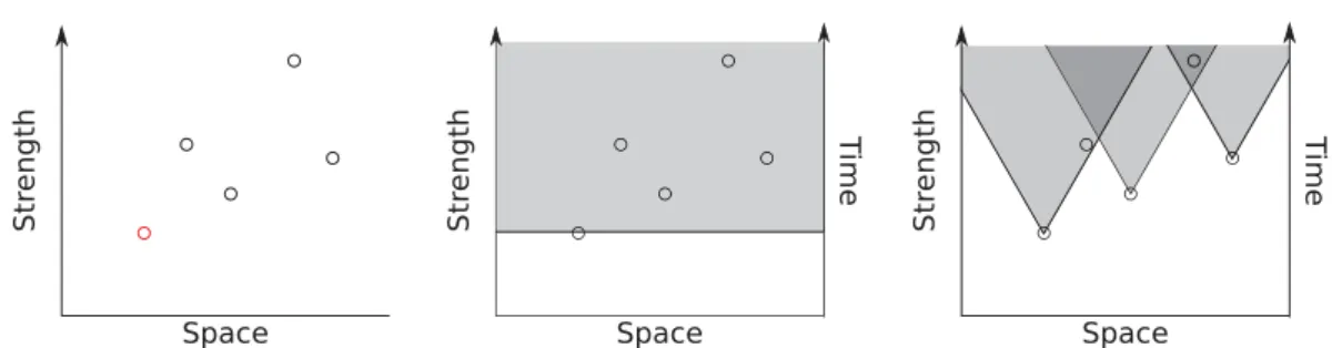
Two failure surfaces are essential for the failure of rock materials (Figure 1.5): the
quasi-static fracture limit and the Hugoniot Elastic Limit (HEL).
At the lowest strain rates (<10
-6s
-1), materials fail under isothermal conditions at
relatively low stresses equal or less than the quasi-static fracture limit. Subcritical crack
growth phenomena often play a major role in these conditions. At conventional
labora-tory strain rates (10
-6– 10
-1s
-1) materials show little to no strain rate sensitivity and
fail in a brittle manner at the quasi-static peak strength. The Griffith failure criterion
(or models that have been developed from it) can predict the failure strength relatively
accurately in terms of the activation and propagation of a critical flaw or a population
of flaws (section 4.1).
At intermediate to high strain rates (10
-1– 10
4s
-1) the failure strength is strongly
1.3 Coseismic off-fault damage by analogous laboratory experiments
S tr ess Strain rate (s-1) 10-6 10-4 10-2 100 102 104 106 quasi-static fracture strength HELsub-critical crack growth
plastic deformation mechanisms mat eria l streng th fracture-kinetics controlled damage S er v o -h ydr aulic machines Pneum.-h ydr . and dr op -w eigh t machines Split Hopk inson P ressur e Bar P la te impac t e xper imetns
isothermal quasi-isothermal adiabatic
ISR HSR UHSR
Quasi-static
Figure 1.5: Failure strength of materials for a broad range of strain rates. The strain rate
values are broadly applicable to geological materials at or near the surface. Two different failure
horizons are crucial: the quasi-static strength and the Hugoniot Elastic Limit (HEL). Four
failure regimes are indicated: sub-critical crack growth, quasi-static failure, fracture-kinetics
controlled failure and shock-related plastic failure mechanisms. A suitable experimental loading
apparatus is indicated for the various strain rates. The appropriate terms for the strain rate
testing fields are: ISR = Intermediate Strain Rate, HSR = High Strain Rate, UHSR = Ultra
High Strain Rate. Figure based on Grady [1998]; Zhang and Zhao [2013a]
due to inertia effects, which affect the fracture kinetics and allow transient loads or stress
waves to exceed the quasi-static fracture limit (Figure 1.5). Due to this time-dependence
of fracturing, several additional fractures have time to develop in addition to the weakest
flaws, leading to a more diffuse fracture pattern. Models explaining fracturing within
this fracture-kinetics controlled regime are discussed in Section 4.
Once the inertial fracture delay has exceeded a certain threshold with respect to the
loading rate (strain rates > 10
4– 10
5s
-1) the material can go beyond the second failure
surface: the HEL (Figure 1.5). Above this elastic limit, a range of alternative failure
mechanisms are activated, such as crystal plasticity and formation of micro-shear zones
filled with nano-particles [Grady, 1998]. Moreover, the adiabatic conditions can result
in local melting, leading to a drastic drop in the rock friction coefficient [Di Toro et al.,
2004]. Effectively, the HEL represents a high strain rate version of the brittle-ductile
transition. The HEL is slightly sensitive to insensitive to changes in strain rate [Grady
et al., 1977; Grady, 1998].
Since the pulverized rocks observed in the field lack plastic deformation and partial
melting, loading conditions close to and beyond the HEL are unlikely to cause
pulver-ization. The pervasive fracture textures suggest that the pulverized rock forms in the
fracture-kinetics-controlled strain-rate-strength domain (Figure 1.5). Experiments in
this strain rate range involve the Intermediate Strain Rate (ISR, strain rate 10
-1– 10
1s
-1) and High Strain Rate (HSR, strain rate 10
1– 10
4s
-1) testing fields [Zhang and Zhao,
2013a]. For ISR testing, pneumatic-hydraulic and drop-weight machines can be used, for
HSR testing the most commonly used apparatus is the Split-Hopkinson Pressure Bar.
This apparatus can be adjusted so that it includes the strain rate range of drop-weight
machines, extending its range to lower strain rates of 10
0s
-1. It has been used in all
studies on pulverized rocks up to date.
1.3.2
Coseismic damage by compressional loading experiments
The Split-Hopkinson Pressure Bar (SHPB) apparatus (also known as Kolsky-bar) was
developed in its current form by Kolsky [1949]. Given the relative novelty of this machine
and its importance in all studies that have been performed up to date, the following
sec-tion covers the basics of the apparatus. Specific attensec-tion is given to the manipulasec-tion of
the imposed compressional stress wave. The current state-of-the-art on dynamic loading
experiments in relation to pulverized rocks is then summarized and discussed.
1.3.2.1
Methodology of the Split-Hopkinson Pressure Bar apparatus
Setup and mechanical history by 1D-wave analysis
A typical SHPB setup includes an input bar and an output bar supported by
low-friction ball bearings or Teflon-coated uprights (Figure 1.6a, b). The rock sample is
placed between the two bars and can be held in place by a lubricant. A launch mechanism
(gas gun, spring gun) accelerates a striker towards the input face of the input bar. The
velocity of the striker depends on the launch mechanism, a spring gun produces lower
velocities and is used to perform reproducible tests at lower strain rates (10
0-10
3s
-1)
than a gas gun (10
2-10
4s
-1). At impact, a compressive planar stress wave is created that
travels through the input bar (Figure 1.6a). Typically the wave has a duration of less
than 1 millisecond. This incident wave splits into a reflected wave and a transmitted
1.3 Coseismic off-fault damage by analogous laboratory experiments
A’ A
launched striker
input bar output bar
sample
strain gage strain gage laser velocimeter
(a)
(c) Raw data record
(d) 150 50 250 -2 0 1 x 10⁻⁴ Strain -3 -1 time (µs) incident reflected transmitted 500 1000 1500 2000 2500 3000 -2 0 2 x 10⁻⁴ Strain Time (µs)
output bar strain gage input bar strain gage
Isolated waves after time shift
sample
input bar L output bar
S AS F I FT F R A B ε T ε I ε R v 1 v2 EB , cB E B , cB incident reflected transmitted time A’ A’ A A (b) 1.25 m (e)
Figure 1.6: (a) Sketch of a typical Split-Hopkinson Pressure Bar (SHPB), in this case a
mini-SHPB with a spring gun as launching system. The velocimeter records the speed of the striker
bar and triggers the data acquisition system. Strain gages record the incident (blue), reflected
(green) and transmitted (red) stress waves as they travel along the length of the bars as indicated
by the three time snapshots. A-A’ indicates the time interval highlighted in gray in figure (c).
(b) Photograph of a mini-SHPB apparatus at the ISTerre laboratory in Grenoble. (c) Raw data
record of the input bar (black) and output bar (black dashed). The gray area corresponds to
A-A’ in figure (a) and encompasses the primary passing of the three stress waves, which are
highlighted in color. The record shows no second loading because the transmitted and reflected
waves do not show a sharp alteration in shape and intensity. (d) The incident, transmitted and
reflected waves after the time shift from the gage locations to the bar interface. (e) Sketch of
the sample and sample-bar interfaces with the bar properties and the direction of strain pulses,
particle velocities and forces. See text and equations A.1-A.6. Figures (c) and (d) show a test
during which a quartz-monzonite sample was deformed in the elastic regime.
wave at the input bar-sample interface (Figure 1.6a). The reflected wave travels back
through the input bar, the transmitted wave travels through the sample and into the
output bar (Figure 1.6a). Both transmitted and reflected waves then travel end-to-end
in their respective bars.
In order to obtain the full stress-strain loading history, the propagation of the planar
stress waves is recorded first. For this purpose, strain gages are placed on the input and
output bars (Figure 1.6a). The acquisition frequency of the gages must be sufficiently
high to ensure that the stress wave loading is monitored in acceptable detail (e.g. a
frequency of 1-2MHz). The strain gages are placed on the bars at specific distances
from their extremities so that the incident, reflected and transmitted waves are recorded
without overlap.
The raw data record is then pre-processed by identifying the first passage of the
three waves (incident, reflected and transmitted, Figure 1.6c). The first two waves
are recorded on the input bar, where by definition the first signal is the incident wave
and the remaining signals are the back-and-forth travelling reflected wave. The output
bar contains exclusively the transmitted wave signal. Only the primary recordings of
the reflected and transmitted waves are needed. The equation describing stress wave
propagation along a thin bar is known as the Pochhammer-Chree equation [Graff, 1991],
so that the three waves can be numerically projected backward (transmitted and reflected
wave) and forward (incident wave) to the edges of the bars, and hence to the edges of
the sample (Figure 1.6d).
The loading history is obtained by applying a 1D-wave analysis [Graff, 1991; Chen
and Song, 2011]. The stress history is obtained by resolving the forces acting on the
bar-sample interfaces for each wave (Figure 1.6e) (subscript I, R and T for incident,
reflected and transmitted wave respectively). The force F is given by:
F
I/R/T= −E
BA
B× ǫ
I/R/T(1.1)
where E
Bis the Young modulus of the bar material, A
Bthe surface area of the bar
extremities and ǫ the strain gage data of the stress wave (the minus sign comes from the
convention that the dilatational strain recorded by a strain gage is positive). The stress
(σ) acting on the surfaces of the sample is computed as a simple force balance divided
by the surface area of the sample (A
S). For the sample output surface this is:
σ
out= −
F
TA
S= −
E
BA
BA
S(ǫ
T)
(1.2)
And for the input surface:
σ
in= −
F
I+ F
RA
S= −
E
BA
BA
S(ǫ
I+ ǫ
R)
(1.3)
Note that the reflected wave has an opposite (tensional) strain, and is thus effectively
subtracted from the incident wave. Equations A.2 and A.3 are called the 1-wave analysis
and 2-wave analysis, respectively. If the assumption of stress equilibrium along the length
1.3 Coseismic off-fault damage by analogous laboratory experiments
of the sample is satisfied, a 3-wave analysis yields the mean stress on the sample:
σ
mean= −
F
I+ F
R+ F
T2A
S= −
E
BA
B2A
S(ǫ
I+ ǫ
R+ ǫ
T)
(1.4)
However, in practice initial stress equilibrium issues render the 2-wave and 3-wave
anal-yses less reliable. Use of the 1-wave analysis is recommended for testing brittle samples.
Strain and strain rate are computed from the relative difference in particle
veloc-ities of the input bar-sample interface (v
1) and the output bar-sample interface (v
2)
(Figure 1.6e). These velocities are given by:
v
1= c
Bd(−ǫ
I+ ǫ
R)
v
2= −c
Bdǫ
T(1.5)
where c
Bd
is the P-wave velocity of the bar material. The relative difference in velocity
divided by the sample length (L
S) then gives the strain rate:
˙ǫ =
v
1− v
2L
S=
c
B dL
S(−ǫ
I+ ǫ
R+ ǫ
T)
(1.6)
A time integration of equation A.6 gives the strain. For more details on 1D-stress
anal-ysis, see Graff [1991]; Gama et al. [2004]; Chen and Song [2011].
Assumptions and pitfalls of 1D-wave analysis
To ensure a valid 1D-wave analysis for brittle samples, the following assumptions must
be verified [Zhao and Gary, 1996; Gama et al., 2004; Chen and Song, 2011; Zhang and
Zhao, 2013a]:
1. The stress wave propagation in the bar is 1D and longitudinal to the bar axis.
2. Stress is in equilibrium along the length of the sample during deformation.
3. Friction and radial inertia effects are kept minimal.
4. The sample is loaded once per test.
1D longitudinal wave propagation: Since the deformation history is obtained by
1D-wave analysis, this assumption is imperative. However, in an experimental setup there are
always small alignment issues so that the bar interfaces are not perfectly perpendicular to
the stress wave propagation direction. Carefully aligning and calibrating the apparatus
before an experiment reduces this error. Keeping the length/diameter ratio of the bars
greater than 20 and input wave stresses below the elastic limit of the bar can further
ensure 1D wave propagation.
The finite diameter of the bars causes dispersion of the stress waves in the bar by
the appearance of multiple propagation modes [Graff, 1991]. This will affect especially
the higher frequency components in the stress wave, which will travel more slowly than
the lower frequency components. Thus, the stress wave measured at the strain gage is
different from the actual stress wave at the bar-sample interfaces. This dispersion can
be described by the Pochhammer-Chree equations [Graff, 1991] and since in practice
only the first propagation mode is activated, the stress wave dispersion can be modeled
relatively easily. From this, the stress wave is corrected for the position at the sample-bar
interfaces.
Stress equilibrium along the length of the sample: This assumption must be valid for
the three-wave stress analysis to be applied. Also, a sample in stress disequilibrium might
result in heterogeneous deformation: for instance, the input side of the sample might be
fractured while the stress at the output side of the sample never exceeds the elastic
limit. Given that, at the onset of loading, a sample is always in stress disequilibrium
for the duration of a ‘ring-up’ period or equilibrium time [Nemat-Nasser et al., 1991;
Zhang and Zhao, 2013a], it is crucial to know the stress level when equilibrium has been
reached. Typical equilibrium times are at least 4 times the transit time [Ravichandran
and Subhash, 1994] or πtimes the transit time [Davies and Hunter, 1963]. The transit
time is the one-way P-wave travel time through the sample.
A simple model can be used to check whether a loading has been in stress equilibrium
before non-elastic deformation has set in, based on linear elastic behavior and wave
reflections [e.g. Ravichandran and Subhash, 1994]. In such models, the expected elastic
behavior is then compared to the actual loading history and the necessary adjustments
can be made for further testing. The input data for such models are the bar material
properties, sample length and an estimate of the density and P-wave velocity of the tested
material. Analysis of these models shows that the sample length, impedance mismatch
between bar and specimen and, most importantly, the shape of the incident pulse in the
early stages of loading, influence the equilibrium time. The manipulation of the incident
pulse is discussed in detail in the next section.
Friction and radial inertia effects: A lubricant at the bar-sample interface can reduce
friction at this interface. During dynamic loading, radial inertia gives rise to extra
axial stress components and therefore results in radial confinement. This effect can
be minimized by keeping the length/diameter ratio of the sample less or equal to one
[Gama et al., 2004; Chen and Song, 2011; Zhang and Zhao, 2013a]. With increasing
1.3 Coseismic off-fault damage by analogous laboratory experiments
sample diameter the radial and axial stress components increase [Forrestal et al., 2007;
Chen and Song, 2011], thus samples with a small diameter experience less inertia-related
additional stress components.
Single loading per test: A second loading during a single test may be preferred in
some cases but increases the difficulty in performing the 1D-wave analysis preprocessing
due to wave overlapping. The occurrence of a second loading can be checked from the raw
data record: the transmitted and reflected waves would record a sudden change in shape
and amplitude in such a case. The risk of this happening can be reduced by installing
a momentum trap [Zhang and Zhao, 2013a] or reducing the length of the output bar so
that it moves away from the sample before reloading from the input bar.
Manipulation of the incident stress wave
Loading conditions of a high strain rate test are defined by the stress magnitude, the
loading duration and the loading rate of the incident wave. A “standard” incident wave
created by the impact of two similar bars is trapezium shaped. Here, we discuss how to
manipulate this trapezium shaped wave so that a reliable high strain rate test can be
designed.
The magnitude of the incident wave determines the stress on the sample. The most
straightforward way to adapt this is by changing the speed of the striker at impact
(Figure 1.7a). A good approximation of the stress magnitude in an incident wave is
given by the following equation for the impact of two similar bars [Graff, 1991]:
σ =
ρ
Bc
B d

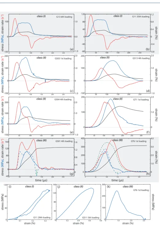
![Figure 1.9: (a): Mechanical data of a fragmented (left) and a pulverized (right) quartz- quartz-monzonite sample [from Aben et al., 2016]](https://thumb-eu.123doks.com/thumbv2/123doknet/14493364.717985/41.892.173.701.193.796/figure-mechanical-fragmented-pulverized-quartz-quartz-monzonite-sample.webp)
![Figure 1.16: Particle motion fields for different rupture velocities (bottom right corner) in a homogeneous elastic material [adjusted from Mello et al., 2010]](https://thumb-eu.123doks.com/thumbv2/123doknet/14493364.717985/62.892.152.759.155.372/figure-particle-different-rupture-velocities-homogeneous-material-adjusted.webp)